利用時間序列之微陣列基因表現資料來比較人類和老鼠在心臟胚胎發育的關係

全文

(1)國立交通大學生物資訊研究所碩士論文. 利用時間序列之微陣列基因表現資料來比較人類和老鼠在心臟胚胎發育的關係 Comparing Fetal Heart Development between Human and Mouse based on Time-Series Gene Expression Profiles. 研究生：任冠樺指導教授：黃憲達博士. 中華民國九十六年六月.

(2) 利用時間序列之微陣列基因表現資料來比較人類和老鼠在心臟胚胎發育的關係 Comparing Fetal Heart Development between Human and Mouse based on Time-Series Gene Expression Profiles. 研究生：任冠樺. Student：Kuan-Hua Jen. 指導教授：黃憲達. Advisor：Hsien-Da Huang. 國立交通大學生物資訊研究所碩士論文. A Thesis Submitted to Institute of Bioinformatics College of the Biological Science & Technology National Chiao Tung University in partial Fulfillment of the Requirements for the Degree of Master in Bioinformatics June 2007 Hsinchu, Taiwan, Republic of China. 中華民國九十六年六月.

(3) 利用時間序列之微陣列基因表現資料來比較人類和老鼠在心臟胚胎發育的關係. 學生：任冠樺. 指導教授：黃憲達. 國立交通大學生物資訊研究所碩士班. 中文摘要心臟的發育是非常複雜的一個生理機制，有非常多的基因在心臟胚胎發育過程參與其細胞調控並決定了心臟的形成。微陣列（基因晶片）的實驗能夠一次大量產生許多基因表現的數據，在此研究中，想利用此一技術產生關於心臟發育時期的基因表現值。由於相關法令的問題，人類心臟胚胎的檢體獲取非常不易。為了更了解關於心臟發育的機制，故也利用老鼠心臟發育的胚胎來建立一個人類和老鼠的在心臟發育方面時間序列的平台。目前大部分的研究人員都使用一種物種來研究發育時期基因的變化，我們特別利用人類與老鼠心臟發育胚胎的時間序列檢體，並且使用兩物種間的同源基因和 dynamic time warping 演算法將此兩種物種作同源基因的分析，找出人類和老鼠中同源基因有相似變化的基因。而後再利用這些基因，做進一步的系統化分析，探討其功能和交互關係。此研究目的就是希望能利用基因表現的數據來更了解心臟發育過程中基因表現的模式與變化，並希望能發掘尚未被先前研究所探討的發育調控基因。. i.

(4) Comparing fetal heart development between human and mouse based on time-series gene expression profiles. Student：Kuan-Hua Jen. Advisors：Dr. Hsien-Da Huang Advisors：. Institute of Bioinformatics National Chiao Tung University. Abstract Heart development is a complex process involving many genes which control cell behavior in the embryo and determine its pattern, its form, and much of its behavior. Microarray experiments can generate an enormous amount of data at one time, so we use this technology to obtain gene expression profiles in heart embryonic development. But it is usually very difficult to obtain human heart fetus sample because of the issues of ethical, legal, and social consideration. In order to help us get more understanding of human heart development, we can use the mouse model system that is most often used. Therefore, we must establish a mapping system to make a cross bridge between these two species on developmental stages. To date, the vast majority of researches have focused their study on one species. Specially, we utilize orthologous genes and incorporate the dynamic time warping algorithm in order to map the time points that human and mouse gene expression profiles having highly correlated pattern. Firstly, we apply the algorithm to select the best time-warped orthologous genes having similar pattern. Then, these genes are clustered into groups. Each group has its unique mapping pattern and different biological meaning. The following task is to find relationship and pattern in distinct groups of genes, and to get close understanding into molecular process and gene function, mechanisms of embryogenesis of the heart, and comparative genomics. Ultimately, our aim is to achieve new insights into the heart developmental biology.. ii.

(5) Acknowledgements. For my parents, and my dear friends. Echo Jen 2007.7. iii.

(6) Table of Contents 中文摘要 ................................................................................................................ i Abstract .................................................................................................................ii Acknowledgements ..............................................................................................iii Table of Contents.................................................................................................. iv List of Figures ...................................................................................................... vi List of Tables ....................................................................................................... vii Chpater 1 Introduction ......................................................................................... 1 1.1 Affymetrix Gene Chip Microarray ............................................................................... 1 1.2 Heart Development.......................................................................................................2 1.3 Experimental Objectives ..............................................................................................4. Chpater 2 Materials and Methods........................................................................ 6 2.1 Materials .......................................................................................................................6 2.1.1 Microarray Datasets...........................................................................................6 2.1.2 Datasets from GEO Database ............................................................................6 2.2 Methods ........................................................................................................................7 2.2.1 Microarray Experiment .....................................................................................7 2.2.1.1 Collection of Human Specimens ............................................................7 2.2.1.2 Animal Experiment.................................................................................7 2.2.1.3 RNA Extraction and Microarray Analysis..............................................8 2.2.2 Data Preprocessing ............................................................................................8 2.2.2.1 Normalization .........................................................................................8 2.2.2.2 Use of replicate data ...............................................................................9 2.2.2.3 Data Filtering........................................................................................10 2.2.2.4 Standardization .....................................................................................10 2.2.2.5 Identification of Orthologous Genes .................................................... 11 2.2.3 Analysis of Gene Expression Data ..................................................................12 2.2.3.1 Distance Similarity Measurements.......................................................13 2.2.3.1.1 Euclidean Distance ....................................................................13 2.2.3.1.2 Pearson Correlation Distance ....................................................13 2.2.3.2 Clustering .............................................................................................14 2.2.3.2.1 Hierarchical Clustering..............................................................15 2.2.3.2.2 K-means Clustering ...................................................................15 2.2.3.3 Software and Tool.................................................................................17 2.2.3.3.1 Genesis ......................................................................................17 2.2.3.3.2 R ................................................................................................17 2.2.3.3.3 RMAExpress .............................................................................18 2.2.3.3.4 MetaCore ...................................................................................18 2.2.4 Time Series Data Analysis...............................................................................18. iv.

(7) 2.2.4.1 The Concept of Time-Warping .............................................................19 2.2.4.2 Time-Warping Programs.......................................................................20. Chpater 3 Results ............................................................................................... 21 3.1 Large-scale transcriptional analysis of the developing heart......................................21 3.2 Construction the Mapping System of Human and Mouse Microarrays .....................22 3.2.1 Time-Warping for the Orthologous Genes ......................................................22 3.2.2 K-means Clustering of Time-Warped Genes into Distinct Groups .................24 3.3 Time Warping for Each Cluster ..................................................................................28 3.4 Functional Distribution of the Best 250 Time-Warped Genes ...................................43 3.5 Finding Statistically Overrepresented GO terms........................................................ 44 3.5.1 P-value Function..............................................................................................45 3.6 Analysis of Transcriptional Regulations.....................................................................50 3.6.1 Transcription Factors in Clusters.....................................................................50 3.6.2 Transcription Factors Regulations ...................................................................51 3.7 Promoter Analysis of the Gene Groups ......................................................................55 3.8 Validation of the discovery by referring to previous works .......................................57 3.8.1 TGF and Wnt family ........................................................................................57 3.8.2 GATA-4 ...........................................................................................................58 3.9 Comparison to GEO Data...........................................................................................59 3.9.1 Human Data vs. GEO Mouse data ..................................................................59 3.9.2 Mouse Data vs. GEO Mouse data ...................................................................59. Chpater 4 Discussions........................................................................................ 61 4.1 Study limitations.........................................................................................................61 4.2 Prospective works.......................................................................................................61 4.2.1 Analyzing Gene Expression Profiles of Human and Mouse among Different Tissues during Embryonic Development..................................................................61 4.2.2 Determination of Abnormal Genes in Development .......................................62 4.2.3 Validation of the role of candidate genes during development using conditional gene knock-out mouse model ................................................................62 4.2.4 Multiple Alignment and Local Alignment.......................................................63 4.3 Conclusion ..................................................................................................................63. Bibliography........................................................................................................ 63 Appendix A.......................................................................................................... 66 Appendix B ......................................................................................................... 79. v.

(8) List of Figures Figure 1.1 Affymetrix GeneChip Array. ................................................................................2 Figure 1.2 Formation of the heart. .........................................................................................4 Figure 2.1 Normalization result of human data. ....................................................................9 Figure 2.2 Normalization result of mouse data. ....................................................................9 Figure 2.3 The overview of the microarray data analysis between human and mouse on the developmental stages. ...................................................................................................12 Figure 2.4 Hierarchical tree. ................................................................................................15 Figure 2.5 K-means clustering.............................................................................................16 Figure 2.6 The concept of time warping..............................................................................19 Figure 3.1 Time warping results of CBX5 and cbx5. ..........................................................23 Figure 3.2 The distance score of 3490 orthologous genes pairs from the minimum to the maximum. 25 Figure 3.3 The distribution of distance scores of the 3490 orthologous gene pairs. ...........26 Figure 3.4 K-means clustering of Human and Mouse 250 genes........................................28 Figure 3.5 Flowchart of applying dynamic time-warping as a step. ...................................30 Figure 3.6 Grouped time warping results and gene networks in the individual group........42 Figure 3.7 FatiGO result for the 250 genes in Level-3 Gene Ontology distribution...........44 Figure 3.8 Transcription factors in cluster 4........................................................................52 Figure 3.9 Transcription factors in cluster 7........................................................................53 Figure 3.10 Transcription factors in cluster 8......................................................................54 Figure 3.11 Transcription factors in cluster 10 ....................................................................55 Figure 3.12 The analyzing flowchart of extracting promoter sequences and scanning TF binding site. 56 Figure 3.13 The detected targets of STAT3 transcription factor. .........................................57 Figure 3.14 Expressions of 62 overlapped genes. ...............................................................59 Figure 3.15 Expressions of 37 overlapped genes. ...............................................................60. vi.

(9) List of Tables Table 2.1 Microarray datasets using in the research. .............................................................6 Table 2.2 Microarray datasets from GEO using in the research. ...........................................7 Table 2.3 Gene expression data matrixⅠ. ........................................................................... 11 Table 2.4 Gene expression data matrixⅡ. ........................................................................... 11 Table 3.1 Preprocessing of the microarray data and the number of genes after many steps of processing. 21 Table 3.2 12 clusters of genes and their numbers and scores in each distinct group...........29 Table 3.3 Biological process that Gene Ontology categories non-randomly enrich in 250 time-warping genes and individual clusters........................................................................45 Table 3.4 Transcription factors in each cluster. ...................................................................50 Table 3.5 Significant biological pathway of 250 Time-warped genes.................................57. vii.

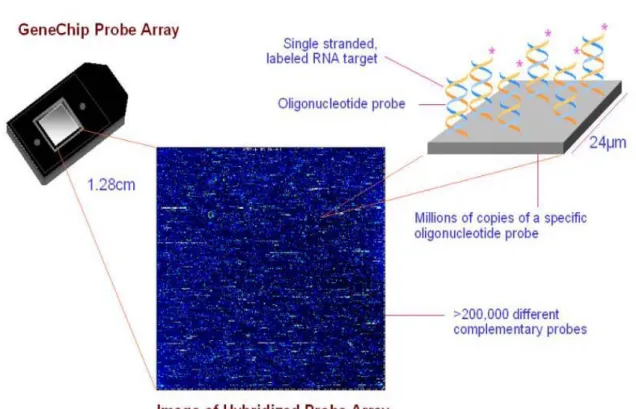
(10) Chpater 1 Introduction 1.1 Affymetrix Gene Chip Microarray In oligonucleotide microarrays (or single-channel microarrays), the probes are designed to match parts of the sequence of known or predicted mRNAs (see in Figure 1.1). There are commercially available designs that cover complete genomes from companies such as GE Healthcare 1 , Affymetrix 2 , Ocimum Biosolutions 3 , or Agilent 4 . These microarrays give estimations of the absolute value of gene expression and therefore the comparison of two conditions requires the use of two separate microarrays. Oligonucleotide Arrays can be either produced by piezoelectric deposition with full length oligonucleotides or in-situ synthesis. Oligonucleotide Arrays are composed of 25-mer or 30-mer and are produced by photolithographic synthesis (Affymetrix) on a silica substrate or piezoelectric deposition (GE Healthcare) on an acrylamide matrix. Oligonucleotide microarrays often contain control probes designed to hybridize with RNA spike-ins. The degree of hybridization between the spike-ins and the control probes is used to normalize the hybridization measurements for the target probes.. 1 2 3 4. GE Healthcare: http://www.gehealthcare.com/worldwide.html Affymetrix: http://www.affymetrix.com/index.affx Ocimum Biosolutions: http://www.ocimumbio.com/web/default.asp Agilent: http://www.home.agilent.com/agilent/home.jspx?cc=US&lc=eng&cmpid=4533. 1.

(11) There are a lot of researches that use the microarray technology to the study of mammalian organogenesis. It can provide great insights into the steps necessary to elicit a functionally competent tissue. Previous researches often focused on maybe one species embryo differentiation [1-3], sex determination of the mammalian gonad [4], gene expression patterns in one organ’s development [5, 6], or analyzing expression profiles during the period from fertilization to implantation [7]. These studies that just mentioned never compare one organ between two species in embryonic development time. Our approach is to synchronize heart development stage between human and mouse and provide an opportunity to identify those functional genes that might be important for controlling embryogenesis and organogenesis.. Figure 1.1 Affymetrix GeneChip Array.. 1.2 Heart Development The heart is the first organ to form during embryogenesis and its function is imperative and intricate from early on for the viability of the mammalian embryos. And it is the one of the few organs that has to function almost it is formed [8]. The developmental mechanisms that control the formation and morphogenesis of this organ have received much attention among classical and molecular embryologists. Due to the evolutionary conservation of many of these. 2.

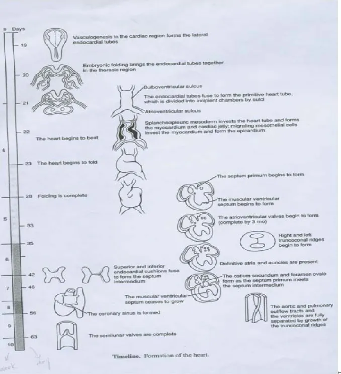
(12) processes, major insights have been gained from the studies of vertebrate model. Heart development in all vertebrates follows the same general pattern: fusion of myocardium and endocardium in the ventral midline to form a simple tubular heart, onset of function, looping to the right side, chamber specification and formation, and at last, development of specialized conduction tissue, coronary circulation, innervation, and mature valves [9] (see in Figure 1.2). Although, many genes important for heart development or organogenesis have been studied for a long time, global analysis of gene expression will provide more information about how the genes work and their interaction networks. In recent years, microarray technology has widely used for researchers to learn how genes’ expression levels in different developmental stages, and to identify the cellular processes in which they participate.. 3.

(13) Figure 1.2 Formation of the heart.. 1.3 Experimental Objectives It is not practical to use multiple fetuses at the same gestational age to obtain statistical significances in gene expression level, because of the scarcity of useable fetal specimens at same gestational age. On the other hand, the change in gene expression along various fetal gestational weeks using the expression profiles derived from one fetus at a gestational age may be misleading, considering the existing variations among individual fetus even at the same age. Therefore, mouse has been adopted as a model system for studies of vertebrate. 4.

(14) development because of its similar features with human and favorable for genetic studies compared with other vertebrate systems. Using the mouse model will allow us to evaluate the changes in gene expression along various developmental stages, because we can use as many mice as necessary for each time point of a gestational age to eliminate the potential variations, which the result only from individual biological variations. After mapping the gene expression profiles with the two species, we choose the best 250 match orthologous genes and cluster these genes into groups. As a preliminary analysis, each group of genes has its unique biological meaning after doing time warping. Moreover, specific characteristics were found to be associated with some features of the gene expression patterns. We employed an integrated analytical approach that encompasses Gene Ontology, biological pathway, and some previous research validations to provide more information for identifying the development-specific genes and get more understanding of their function in cardiogenesis. Our works presents a good example in which the combination of microarray technology with human and mouse model will not only consolidate our existing knowledge, but will also help us to identify novel factors that might be important for organogenesis. It also provides us with a global view on how genes are coordinated to form a genetic network to control heart embryogenesis. The aims of this research are shown as below: 1. Constructing the mapping system between human and mouse 2. Aligning two different time series profiles by using microarray data 3. Identification of heart development-related genes 4. Understanding developmental related genes’ function, pathway, regulation, and how they are coordinated to form a genetic network to control heart embryogenesis 5. Achieve new insights into the heart developmental biology. 5.

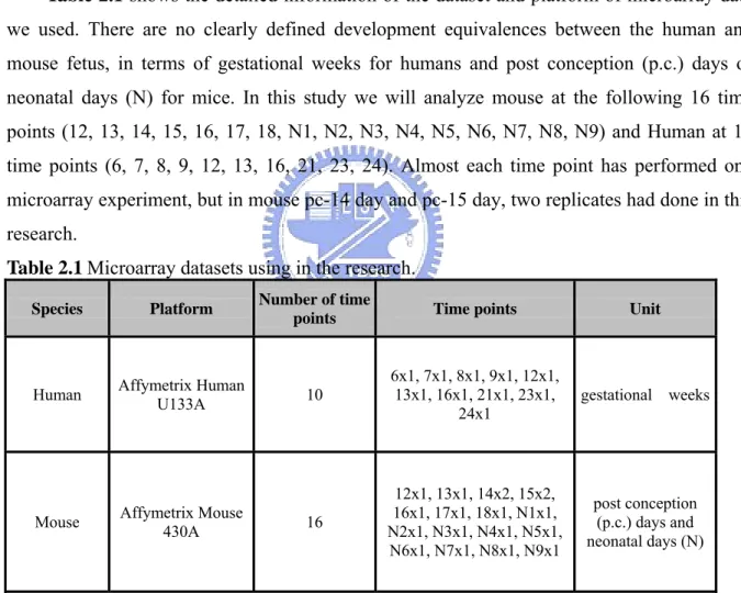
(15) Chpater 2 Materials and Methods 2.1 Materials 2.1.1 Microarray Datasets Affymetrix Human U133A and mouse 430A GeneChips have been successfully processed at the Genomic Medicine Research Core Laboratory (GMRCL) of Chang Gung Memorial Hospital. Table 2.1 shows the detailed information of the dataset and platform of microarray data we used. There are no clearly defined development equivalences between the human and mouse fetus, in terms of gestational weeks for humans and post conception (p.c.) days or neonatal days (N) for mice. In this study we will analyze mouse at the following 16 time points (12, 13, 14, 15, 16, 17, 18, N1, N2, N3, N4, N5, N6, N7, N8, N9) and Human at 10 time points (6, 7, 8, 9, 12, 13, 16, 21, 23, 24). Almost each time point has performed one microarray experiment, but in mouse pc-14 day and pc-15 day, two replicates had done in this research. Table 2.1 Microarray datasets using in the research. Species. Platform. Number of time points. Time points. Unit. Human. Affymetrix Human U133A. 10. 6x1, 7x1, 8x1, 9x1, 12x1, 13x1, 16x1, 21x1, 23x1, 24x1. gestational weeks. Mouse. Affymetrix Mouse 430A. 16. 12x1, 13x1, 14x2, 15x2, 16x1, 17x1, 18x1, N1x1, N2x1, N3x1, N4x1, N5x1, N6x1, N7x1, N8x1, N9x1. post conception (p.c.) days and neonatal days (N). 2.1.2 Datasets from GEO Database There are several public repositories for gene expression data, which, in time, are likely to serve a role for gene expression data similar to that of DDBJ/ EMBL/GenBank for sequence data.. We. found. a. dataset. from. Gene. Expression. Omnibus. (GEO;. http://www.ncbi.nlm.nih.gov/geo/) is also performed in the mouse heart embryonic. 6.

(16) development, and used it to validate our own data. The dataset in GEO is GDS627 (see in Table 2.2). Table 2.2 Microarray datasets from GEO using in the research. Species. Platform. Number of time points. Time points. Unit. Mouse. Affymetrix Mouse 430A (GDS627). 7. 10.5x3, 11.5x3, 12.5x6, 13.5x6, 14.5x6, 16.5x6, 18.5x6. post conception (p.c.) days. 2.2 Methods 2.2.1 Microarray Experiment 2.2.1.1 Collection of Human Specimens Total RNA specimens of human heart from 6th to 12th week of gestational weeks were obtained from ViroGen Inc. (Watertown, MA, USA). Human abortuses of gestational weeks at 13, 16, 20, 21, 23 and 24 were donated by pregnant women with either cervical incompetence or premature preterm rupture of membrane, resulting in inevitable delivery of otherwise normal fetuses. Fetal organs were immediately kept in RNAlater reagent (Ambion, TX. USA) at 4oC for 24-48 h before transferred to –80oC for long term storage. All pregnant women in this study signed an informed consent. This study was approved by the Internal Review Board (IRB) of Chang Gung Memorial Hospital.. 2.2.1.2 Animal Experiment Female C57/BL6 mice at 8 to 10 weeks of were used in this study. In the afternoon, four female mice were transferred to each cage containing one male mouse at 12 to 14 weeks old. On the next morning, each group of 4 female mice were transferred to a new cage and labeled as potentially post conception (PC) day 0. Pregnancy in female mice became visually detectable on PC day 10, and the fetuses were collected on the noon of PC day 12 through PC day 18. For this group of C57/BL6 mice, spontaneous delivery occurred on PC day 19, when the neonates were labeled as the neonate (N) day 0. Neonatal mice were collected from N day 1 to N day 9. Collected through hysterectomy, fetal mice from PC day 12 to 15 were immediately immersed in RNAlater at 4oC for 48 h before organs were collected by dissection under. 7.

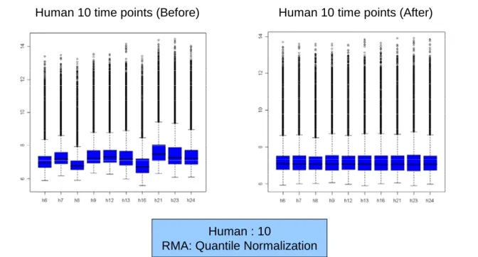
(17) microscopy. Mice at age from PC day 16 through N day 9 were sacrificed by cervical dislocation, and the dissected organs were immersed in RNAlater at 4oC for 48 h before RNA was extracted. Hearts from 4 to 8 fetal mice were pooled at each time point. The use of animal in this study had complied with the guidelines of Experimental Animal Committee and this study was approved by the Internal Review Board (IRB) of Chang Gung Memorial Hospital.. 2.2.1.3 RNA Extraction and Microarray Analysis The procedures of RNA extraction using TRIZOL (Invitrogen, Carlsbad, CA, USA) and RNAeasy purification kit (Qiagen Inc., Valencia, CA,USA), and confirmation of RNA quality and quantity with Agilent Bioanalyzer 2100 (CA, USA) were similar to previous reports [10-13]. Gene expression profiles in human fetal heart and murine heart were analyzed Affymetrix U133A GeneChip and 430A GeneChip, respectively.. 2.2.2 Data Preprocessing 2.2.2.1 Normalization There are a variety of reasons why the raw measurements of gene expression for two samples may not be directly comparable: the quantity of starting RNA may not be equal for each of the samples, there may be differences in labeling and detection efficiencies for the fluorescent labels, and there may be additional systematic effects that can skew the measured expression levels and the derived expression ratios. Normalization is any data transformation that adjusts for these effects and allows the data from two samples to be appropriately compared. Robust Normalization accounts for probe set characteristics resulting from sequence-related factors, such as affinity of the probe set to the RNA and linearity of the hybridization of each probe pair. More specifically, this factor corrects for the inevitable error of using an average intensity of all the probes on the array as a normalization factor for every probe set. Robust Multi-array Analysis (RMA) was adopted due to its sensitivity and specificity in detecting differential expression and is a useful improvement to other kinds of normalization method for researchers using the GeneChip technology [14, 15]. The normalization results are presented in Figure 2.1 and Figure 2.2.. 8.

(18) Human 10 time points (Before). Human 10 time points (After). Human : 10 RMA: Quantile Normalization. Figure 2.1 Normalization result of human data.. Mouse 16 time points with replicates (Before). Mouse 16 time points with replicates (After). Mouse : 18 RMA: Quantile Normalization. Figure 2.2 Normalization result of mouse data.. 2.2.2.2 Use of replicate data Replication is essential for identifying and reducing the effect of variability in any experimental assay, and microarray analysis is no exception. Biological replicated use independently derived RNA from distinct biological sources to provide an assessment of both the variability in the assay and the inherent biological variability in the system under study.. 9.

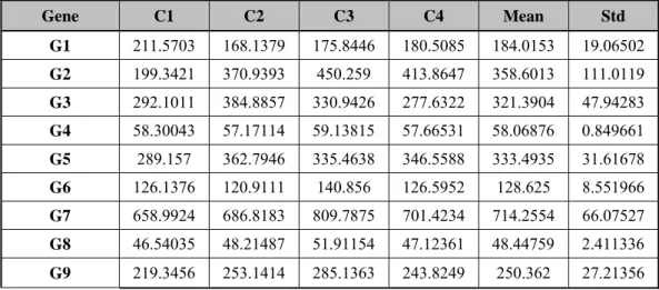
(19) Biological replicates allow commonly expressed genes to be identified, as well as those that are distinct to the particular biological sample. In the research, we did average the replicated to produce a single consensus measurement and thereby reduce the complexity of the final data.. 2.2.2.3 Data Filtering The goal of most other transformations is to filter the dataset to reduce its complexity and increase its overall quality. Many are designed to flag questionable and low quality data, while others are used to identify differentially expressed genes or to enhance particular feature of the data. Below is our method. If more than one probe sets represented the same gene, their intensities were averaged. Then, all hybridization intensity values ﹤20, including negative intensity values, were raised to a value of 20, in order to prevent the too small and negative intensities in these datasets. If the continuous time-points expression profile of one single gene is too flat, we called it “smooth pattern”, that gene would be filtered out. We hope that each gene we use for the latter dynamic time warping algorithm has a specific expression pattern; it means that the gene has variable expression intensities at different developmental ages, and we guess maybe this gene control the embryogenesis and has an important role in heart development. We made the calculation for genes with all the time-point intensities smaller its mean ± 0.3*mean were excluded from the latter use of mapping. As a result, we collected only undulated genes with any intensity of variation of greater than mean ± 0.3*mean, and transformed the data to z-score. Finally, z-score values at transcriptome level were calculated to represent expression data of each gene.. 2.2.2.4 Standardization If a distribution is normal but not standard, we can convert a value to the Standard normal distribution table by first by finding how many standard deviations away the number is from the mean. The number of standard deviations from the mean is called the z-score and can be found by the formula: Z =. x - μ. σ. . Consider the gene expression matrices in Table 2.3 and Table. 2.4. They all represent the expression levels of genes G1-G9 for experimental conditions C1,. C2, C3 and C4. Table 2.3 is the original data and Table 2.4 is the original data transformed into z-score (standardization).. 10.

(20) Table 2.3 Gene expression data matrixⅠ.. Gene expression data matrix of absolute expression measurements after normalization for samples C1, C2, C3 and C4. Gene. C1. C2. C3. C4. Mean. Std. G1. 211.5703. 168.1379. 175.8446. 180.5085. 184.0153. 19.06502. G2. 199.3421. 370.9393. 450.259. 413.8647. 358.6013. 111.0119. G3. 292.1011. 384.8857. 330.9426. 277.6322. 321.3904. 47.94283. G4. 58.30043. 57.17114. 59.13815. 57.66531. 58.06876. 0.849661. G5. 289.157. 362.7946. 335.4638. 346.5588. 333.4935. 31.61678. G6. 126.1376. 120.9111. 140.856. 126.5952. 128.625. 8.551966. G7. 658.9924. 686.8183. 809.7875. 701.4234. 714.2554. 66.07527. G8. 46.54035. 48.21487. 51.91154. 47.12361. 48.44759. 2.411336. G9. 219.3456. 253.1414. 285.1363. 243.8249. 250.362. 27.21356. Table 2.4 Gene expression data matrixⅡ.. Gene expression data matrix of expression measurements after standardization for samples C1, C2, C3 and C4 Gene. C1. C2. C3. C4. G1. 1.445314. -0.8328. -0.42857. -0.18394. G2. -1.43461. 0.111142. 0.825657. 0.497815. G3. -0.61092. 1.324397. 0.199241. -0.91272. G4. 0.272665. -1.05644. 1.258615. -0.47484. G5. -1.40231. 0.926756. 0.062316. 0.413238. G6. -0.29085. -0.902. 1.430197. -0.23734. G7. -0.83636. -0.41524. 1.445807. -0.1942. G8. -0.79095. -0.09651. 1.436528. -0.54907. G9. -1.13974. 0.10213. 1.27783. -0.24022. 2.2.2.5 Identification of Orthologous Genes Orthologs are genes that are related by direct evolutionary descent. The identification of orthologs is particularly important because these genes should play similar developmental or physiological roles, and consequently, their study in rodent or other models can provide insight into their functions in humans. We use orthologous genes to establish relations between human and mouse and then analysis their gene expression profiles with microarray data. HomoloGene is a system for automated detection of homologs among the annotated. 11.

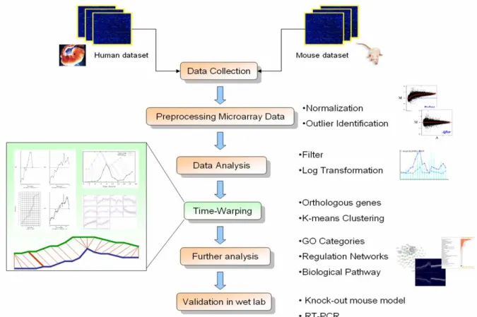
(21) genes of several completely sequenced eukaryotic genomes. The genomes represented in the recent Build 52 of HomoloGene include Homo sapiens, Mus musculus, Rattus norvegicus, Drosophila melanogaster, and so on [16]. This database contains 19157 orthologous genes. between human and mouse. Table 3.1 presents the preprocessing steps and detailed information of the microarray. data we used. We have performed a novel bioinformatics study and use the orthologous genes to be the cross-bridge between human and mouse. At last, we concluded the number of orthologs (probe sets) included in U133A and 430A is around 15530. Therefore, we have a large set of common genes covered by both sets to do the comparative functional genomics study. Figure 2.3 reveals the overview of our analysis of microarray data between human and mouse.. Figure 2.3 The overview of the microarray data analysis between human and mouse on the developmental stages.. 2.2.3 Analysis of Gene Expression Data The goal of microarray data analysis is to find relationships and patterns in the data and ultimately achieve new insights into the underlying biology. For instance, one could look for groups of genes having similar expression under similar conditions and try to find whether their products share similar functional roles in the cell, or for genes whose expression depends. 12.

(22) on the particular state of the system and see if the functions of their products can help to explain the particular phenotype.. 2.2.3.1 Distance Similarity Measurements Most of the gene expression data analysis methods are based on comparisons between the gene or sample expression profiles. In order to make these comparisons first we need a way to measure similarity or dissimilarity between these objects, i.e. between vectors representing genes or samples.. 2.2.3.1.1 Euclidean Distance Euclidean distance is the most common distance measure, and the one we use in everyday situations. Euclidean distance between points A = (a1, a2) and B = (b1, b2) in two dimensions can be expressed using Pythagoras’s theorem: D Eucl (A,B) =. (a1-b1). 2. +. (a 2 -b 2 ). 2. In n-dimensional space for vectors A = (ai,…,an) and B = (bi,…,bn), Euclidean distance can be expressed as : D Eucl (A,B) =. (a i -bi ). 2. 2.2.3.1.2 Pearson Correlation Distance We assume that the arithmetic mean of each gene expression profile is zero. We will see that under this assumption the angle distance is closely related to the Pearson correlation coefficient. The two expression profiles A and B for four samples are given. These are represented by vectors in four-dimensional space: A = (a1, a2, a3, a4) and B = (b1, b2, b3, b4). We can calculate the mean value for each profile as:. a = (a1 +a 2 +a 3 +a 4 )/4 and b = (b1 +b 2 +b3 +b 4 )/4 And shift each profile “down” by its mean, i.e. obtain new vectors: A 0 = (a1 - a, a 2 - a, a 3 - a, a 4 - a) and B0 = (b1 - b, b 2 - b, b3 - b, b 4 - b) Their dot product equals:. 13.

(23) A 0 ⋅ B0 = (a1 - a)(b1 - b) + (a 2 - a)(b2 - b) + (a 3 - a)(b3 - b) + (a 4 - a)(b4 - b) In general, in n-dimensional space: n. A 0 ⋅ B0 = ∑ (a i - a)(bi - b) i=1. If we divide this by n-1, we obtain the well=known expression for covariance, which is used to establish the degree of association between two or more distributions. Covariance is calculated in the same way as variance, except that there are multiple distributions. The variance can be thought of as a measure of the distance from the mean, or the “spread” of the data. Covariance is the generalization of variance for two distributions and can be expressed as: Cov(A, B) =. A 0 ⋅ B0 ( n - 1). The normalized covariance gives the expression for linear correlation, also known as the Pearson correlation coefficient (PCC): A 0 ⋅ B0 Cor(A, B) = 0 A B0. In this way we see that the PCC between vectors A and B is the same as the angle distance between these vectors in normalized and mean centered space. For unrelated distributions the PCC is near 1 for a strong correlation and near zero for a weak correlation.. 2.2.3.2 Clustering The goal of gene expression data clustering is to group together genes or samples that have similar expression profiles. Clustering is currently the most popular method of gene expression matrix analysis. It can be useful for discovering “type” of behavior, for reducing the dimensionality of the data (allowing tens of thousands of genes to be represented by a few groups each containing genes that behave similarly), as well as for the detection of outliers in the data. Clustering is one of the unsupervised approaches to data analysis, which can be used in the absence of a priori information, or when annotations are not considered in the analysis.. 14.

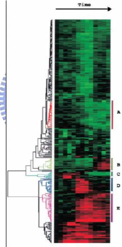
(24) 2.2.3.2.1 Hierarchical Clustering Hierarchical agglomerative clustering is a process in which the data are successively fused, typically until all the data points are included. For hierarchical agglomerative clustering usually all the pair-wise distances between objectives need to be defined. An agglomerative process typically starts by considering each object/data point as a separate, or singleton, cluster. Starting with n objects, the result of the first iteration of clustering is that the two objects that are most similar are grouped together to form a single cluster, leaving (n-1) clusters. The distance between the objects and the newly formed cluster containing two objects is then updated and the next most similar objects and clusters are grouped together as a single cluster[17]. The results of hierarchical clustering are frequently represented in a hierarchical tree, also known as a dendrogram (see in Figure 2.4).. Figure 2.4 Hierarchical tree.. 2.2.3.2.2 K-means Clustering K-means is the most common method of partition-based clustering. It starts with the given number of cluster centers, chosen either randomly or by applying some heuristics. Next the distance from the centroids to every object is calculated, and each object is assigned to the cluster defined by the closest centroid; then, for each cluster the new centroid is found. The distance from each object to each of the new centroids is calculated and in this way the. 15.

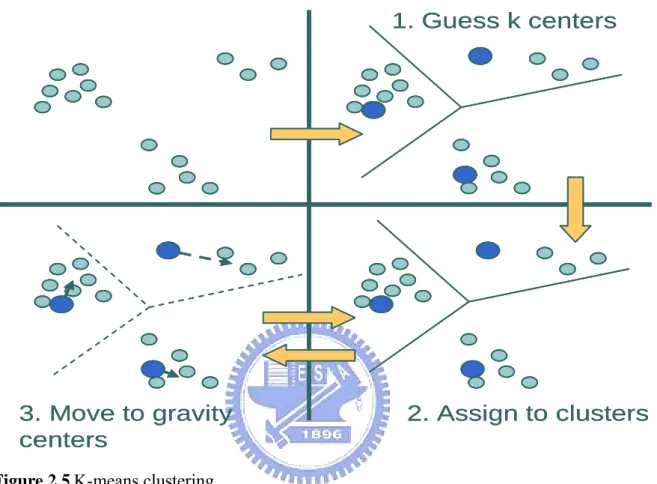
(25) boundaries of the partitioning are revised. This is repeated either until the centroids stabilize or until an a priori defined maximum number of iterations has been reached (see in Figure 2.5).. 1. Guess k centers. 3. Move to gravity centers. 2. Assign to clusters. Figure 2.5 K-means clustering.. 16.

(26) 2.2.3.3 Software and Tool 2.2.3.3.1 Genesis. 2.2.3.3.2 R. 17.

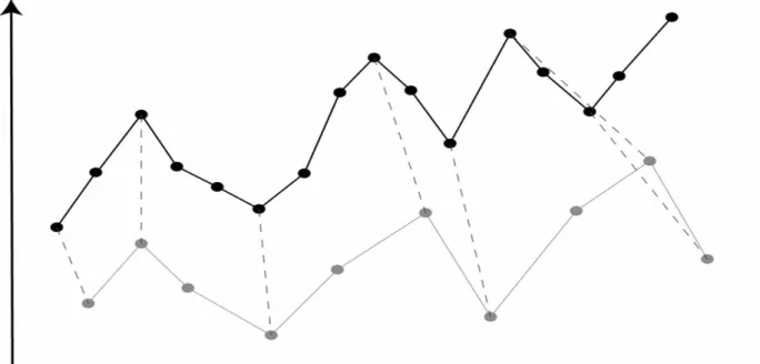
(27) 2.2.3.3.3 RMAExpress. 2.2.3.3.4 MetaCore. 2.2.4 Time Series Data Analysis Time series experiments provide a particular type of gene expression profile, revealing information about the order and the time scale of the expression events. In our research, we wish to compare gene expression time series data from different experiments corresponding to two similar species. An example of such an approach is comparing gene expression during the cell cycle for cell cultures synchronized using time warping [18]. If some of the genes. 18.

(28) involved in the process under study are known, we can “synchronize” the periods, by comparing the expression level of these known genes. Suppose the gene expression profiles of these two species is subject to variation, so that a function may be traced out more slowly during one portion and more quickly during another, and suppose these variations differ from one occasion to another. To allow for such variations when comparing functions, it is necessary to distort or “warp” the time axis appropriately, i.e., compressing it at some places and expanding it at others. The process of inferring the necessary compressions and expansions is often called time-warping [19]. Figure 2.6 demonstrates the concept of time warping.. Figure 2.6 The concept of time warping.. The two time series have different rate of their expression level. In general, we need to use a distance measure, for which the time points of one series can match to the other.. 2.2.4.1 The Concept of Time-Warping Biological processes have the property that multiple instances of a single process may unfold at different and possibly non-uniform rates in different organisms, strains individuals, or conditions. For instances, different individuals affected by a common disease may progress at different and varying rates. This presents an issue for analysis of biological processes using time series of RNA expression levels: To find the time point of one series that corresponds best to that of another, it is insufficient to simply pair off points taken at equal measurement times. Analysis of such time series may therefore benefit from the use of alignment. 19.

(29) procedures that map corresponding time points in different series to one another. An important area of application of these techniques is the study of biological processes that develop over time by collecting RNA expression data at selected time points and analyzing them to identify distinct cycles or waves of expression.. 2.2.4.2 Time-Warping Programs In our research, we have the datasets of the same biological condition which are human and mouse heart on developmental stages. In order to compare these two heart developmental time series in different species, we apply two time warping programs genewarp and grphwarp [18]. genewarp performs a simple time warping and grphwarp is a graphics generation program that take a file produced by genewarp. While genewarp can be used on any set of genes regardless of whether their individual time course expression profiles are similar, we first applied it to all orthologous genes respectively so that they could be aligned. But these orthologous genes maybe don’t have similar profiles; we have to choose the best 250 “mapping genes”. These “250 mapping genes” have two characteristics. Firstly, they are all orthologous gene pairs. Secondly, each pair of them have similar expression pattern after doing “time-warping”. It had been known that genes maybe have different expression patterns during the same biological process. We cluster these 250 genes into distinct groups according to their expression profiles. Therefore, genes in the same cluster have similar expression pattern and maybe the same biological function.. 20.

(30) Chpater 3 Results 3.1 Large-scale transcriptional analysis of the developing heart Approaches using DNA microarray have been successful in studying genome-wild transcriptional regulation during animal development, but suffer from several limitations. On multicellular organisms, cell division and differentiation leads to an increase in tissue complexity throughout development, but whole-animal microarray analysis cannot document this spatial information. We attempt to isolate mRNA form single tissue (Heart) at different developmental stages, measure gene expression, and assign expression to every gene at every time, in order to recreate the entire developmental expression pattern. Affymetrix oligonucleotide microarray platform has been used worldwide more than 1618 reports compiled in the NCBI PubMed Medline, till Jun 2007. The Affymetrix GeneChip system has been requires user to follow a strict manufacture’s protocol. Therefore, Affymetrix system has been considered as a relatively stable platform and proved to be acceptable by the worldwide research community. According to its consistency and comparability of Affymetrix platform, we use U133A for human and 430A for mouse to do this research. Affymetrix Human U133A and mouse 430A GeneChips have been successfully processed at the Genomic Medicine Research Core Laboratory (GMRCL) of Chang Gung Memorial Hospital. Furthermore, we have performed a pilot bioinformatics study and concluded the number of orthologous gene (transform to gene symbol ID) included in these two kinds of commercial GeneChips is around 8578. These orthologous genes are very prominent material to establish a cross-bridge between Human and Mouse. Therefore, we have a large set of orthologous genes covered by both chips to do the comparative functional genomics study. After preprocessing the array data, there has 3490 orthologous genes between human and mouse chip (see in Table 3.1 (b) ). We used these genes for further analysis. Table 3.1 Preprocessing of the microarray data and the number of genes after many steps of processing. Gene Chip. Human Genome U133A. Mouse Genome 430A. 21. Description.

(31) Probe sets. 22283. 22690. Number of probe sets on the chip. Total genes. 13477. 14218. Probe set ID transform to gene symbol. Orthologous genes Non-smooth genes. Overlapped orthologous genes between human and mouse. 8578 (a) 7919. 7934. Filtering flat expression genes. Orthologous genes. 3490 (b). Overlapped orthologous genes between human and mouse. Time Warping. 3490. Single orthologous gene pair time warping. Time Warping. 250. Select 250 genes which distance scores are the least. 3.2 Construction the Mapping System of Human and Mouse Microarrays There are no clearly defined development equivalences between the human and mouse fetus, in terms of gestational weeks for humans and post conception (p.c.) days or neonatal days (N) for mice. Thus, in this study we will analyze mouse at the following 16 time points (12, 13, 14, 15, 16, 17, 18, N1, N2, N3, N4, N5, N6, N7, N8, N9) and Human at 10 time points (6, 7, 8, 9, 12, 13, 16, 21, 23, 24). Table 2.1 shows the detailed information of the dataset and platform of microarray data we used. We use computational methods to provide a novel approach utilizing the gene expression profiles to match these two species with orthologous genes and select the best matching time-points which the expression patterns are highly correlated. Results from this study we propose here will provide the first-in-the-world complete data, at the transcriptome level, about the fetal development equivalence between the human and mouse.. 3.2.1 Time-Warping for the Orthologous Genes Orthologs are genes in different species that have evolved from a common ancestral gene by speciation and generally retain a similar function in the course of evolution. When mapping the expression profiles of human and mouse, using orthologous genes is a good way. In this approach, we use orthologous genes covered by human and mouse affymetrix microarray platform. We do the time-warping for each pair of orthologous gene in order to find their similarity of time series expression data. Time warping considers the similarity of pairs of. 22.

(32) vectors (orthologous gene) taken from a common k-dimensional space (feature space) taken one from each time series. Figure 3.1 illustrates the time warping result of one orthologous gene between human and mouse.. Human CBX5. Mouse cbx5. Alignment. Figure 3.1 Time warping results of CBX5 and cbx5.. CBX5 is a chromobox homolog 5 gene, and its orthologous gene in mouse is cbx5. We got their gene expression profiles by the order of developmental time points. Top-left is the gene expression values of CBX5 in 10 time points; Top-right is the gene expression values of cbx5. 23.

(33) in 16 time points. After applying the dynamic time warping program, genewarp, their expression profiles can map to each other like global alignment. Bottom-left is an alignment grid for CBX5 and cbx5. Every alignment corresponds to a path in the alignment grid from (0, 0) to (n, m). The entire alignment is simply a path (0, 0) →(1, 0) →(1, 1) →(1, 2) →(2, 3) →(3, 4) →(4, 5) →(4, 6) →(5, 6) →(6, 7) →(7, 8) →(7, 9) →(7,10) →(8, 11) →(8, 12) →(8, 13) →(8, 14) →(8, 15) →(9, 15) from (0, 0) to (n, m) in the grid. The score means the similarity of these two time series, the lower the score evaluates; the more similar the two time series are. In this case, the score of these two profiles is 2.51184. Bottom-right is the time alignment of these two profiles.. 3.2.2 K-means Clustering of Time-Warped Genes into Distinct Groups After “warping” for each single orthologous gene, we choose the best similar 250 genes for further analysis. Figure 3.2 demonstrates the distance scores of 3490 othologous gene from minimum to maximum. The fewer the distance score, the more similar the orthologous gene pairs. Figure 3.3 displays the distribution of 3490 orthologous genes. The selected 250 gene pairs have very similar expression pattern after time warping. It means that these genes are co-expressed in human and mouse heart development. These genes have three characteristics: (1) They are all orthologous gene pairs. (2) They are developmental related genes, especially expressed on embryonic stages. (3) After time warping, they have similar expression patterns. We called that “co-expressed gene pairs”. Each “co-expressed gene pairs” have its unique matching time points. In order to know these genes more systematic, we use k-means clustering to divide these 250 genes into 12 groups. In order to make our data more authentic, we combined mouse and human expression data to do the clustering in order to make the human and mouse data more correspondent with each other. After clustering, each group of genes has very similar pattern. Figure 3.4 shows k-means clustering result of the 250 orthologous genes. The annotations of the 250 genes are listed in Appendix A.. 24.

(34) Score 14. 12.8224. 12 10 8 6 4.19951. 4 2 0 1. 400. 799. 1198. 1597. 1996. 2395. 2794. 3193. Gene Order. Figure 3.2 The distance score of 3490 orthologous genes pairs from the minimum to the. maximum. The minimum score of gene (FZD2) is 2.35004; and the maximum score of gene (FLJ10847) is 12.8224. We select the most similar 250 genes which distance scores are less than about 4.2, and use these genes for further analysis.. 25.

(35) # of genes 1400 1200 1000 800 600 400 200 0 2. 3. 4. 5. 6. 7. 8. 9. 10. 11. 12 Distance score. Figure 3.3 The distribution of distance scores of the 3490 orthologous gene pairs.. Most genes’ scores are less than 6 and more than 5. There are just two gene’s distance scores more than 12.. 26.

(36) a 1. 2. 3. 4. 5. 6. 7. 8. 9. 10. 11. 12. H1. H2. H3. H4. H5. H6. H7. H8. H9. H10. H11. H12. b. 27.

(37) c M1. M2. M3. M4. M5. M6. M7. M8. M10. M11. M12. M9. Figure 3.4 K-means clustering of Human and Mouse 250 genes.. (a) K-means clustering of combining human and mouse 250 genes expression values. First 16 time points are the mouse values; Last 10 time points are the human values. Each box illustrates the expression values (log2 ratio) of genes in this group and how many genes clustering into this group. (K=12 and the distance measurement is Pearson correlation coefficient). (b) The 12 groups of human 250 genes. (c) The 12 groups of mouse 250 genes correspondent to their human orthologous genes. Each group of genes has the similar expression trend with their correspondent human group so it is very appropriate for the next step---time-warping within the same group of genes between human and mouse.. 3.3 Time Warping for Each Cluster Each cluster contains many genes, which have similar expression patterns. Figure 3.4 show the expression profiles of 250 genes in 12 clusters between human and mouse. We therefore implemented time warping algorithm for each group of genes between human and mouse, and. 28.

(38) hypothesize that genes in the same cluster group have the same biological functions. Table 3.2 clarifies the distance score and gene number of each cluster. At last, each cluster has its. unique time points mapping pattern. In this approach, we want to find many different gene expression patterns on heart developmental stages and make a pilot study for the research of human and mouse heart development. Detailed information of each group after time-warping is provided in Appendix B. Figure 3.5 clarifies the system flow of our approach using dynamic time-warping. Figure 3.6 exhibits gene expression profiles and time-warping results in the 12 distinct clusters. Table 3.2 12 clusters of genes and their numbers and scores in each distinct group. Mouse Cluster. Human Cluster. Number of Genes. Score. M1. H1. 11. 30.2521. M2. H2. 14. 35.6842. M3. H3. 16. 34.3911. M4. H4. 37. 55.5629. M5. H5. 3. 11.5195. M6. H6. 22. 43.2182. M7. H7. 35. 50.6715. M8. H8. 49. 68.406. M9. H9. 9. 25.9278. M 10. H 10. 38. 53.0934. M 11. H 11. 9. 30.3447. M 12. H 12. 7. 26.919. 29.

(39) Figure 3.5 Flowchart of applying dynamic time-warping as a step.. Firstly, single orthologous gene pair is applied the time warping step. After that, we selected the best genes which are warped great. Next step, the k-means clustering is used to clustering the best warped genes. The last step is to time-warp each cluster of genes individually.. 30.

(40) Cluster 1. Human. Human. Mouse. Mouse. 6. 7. 8. 9. 12. 13. 16. 21. 23. 24. 12 13 14 15 16 17 18 N1 N2 N3 N4 N5 N6 N7 N8 N9. No. of human genes. 11. No. of mouse genes. 11. Distance. 31. 30.2521.


(42) Cluster 3. Human. Human. Mouse. Mouse 6. 7. 8. 9. 12. 13. 16. 21. 23. 24 12 13 14 15 16 17 18 N1 N2 N3 N4 N5 N6 N7 N8 N9. No. of human genes. 16. No. of mouse genes. 16. Distance. 33. 34.3911.

(43) Cluster 4 Human. Mouse Human. Mouse 6. 7. 8. 9. 12. 13. 16. 21. 23. 24. 12 13 14 15 16 17 18 N1 N2 N3 N4 N5 N6 N7 N8 N9. No. of human genes. 37. No. of mouse genes. 37. Distance. 34. 55.5629.


(45) Cluster 6. Human Human. Mouse. Mouse. 6. 7. 8. 9. 12. 13. 16. 21. 23. 24. 12 13 14 15 16 17 18 N1 N2 N3 N4 N5 N6 N7 N8 N9. No. of human genes. 22. No. of mouse genes. 22. Distance. 36. 43.2182.

(46) Cluster 7 Human. Mouse. Human. 6. 7. 8. 9. 12. 13. 16. 21. 23. 24 12 13 14 15 16 17 18 N1 N2 N3 N4 N5 N6 N7 N8 N9. Mouse. No. of human genes. 35. No. of mouse genes. 35. Distance. 37. 50.6715.

(47) Cluster 8 Human. Mouse Human. Mouse 6. 7. 8. 9. 12. 13. 16. 21. 23. 24. 12 13 14 15 16 17 18 N1 N2 N3 N4 N5 N6 N7 N8 N9. No. of human genes. 49. No. of mouse genes. 49. Distance. 38. 68.406.

(48) Cluster 9. Human. Mouse. Human. Mouse. 6. 7. 8. 9. 12. 13. 16. 21. 23. 24. 12 13 14 15 16 17 18 N1 N2 N3 N4 N5 N6 N7 N8 N9. No. of human genes. 9. No. of mouse genes. 9. Distance. 39. 25.9278.

(49) Cluster 10 Human. Mouse Human. 6. 7. 8. 9. 12. 13. 16. 21. 23. 24. Mouse. 12 13 14 15 16 17 18 N1 N2 N3 N4 N5 N6 N7 N8 N9. No. of human genes. 38. No. of mouse genes. 38. Distance. 40. 53.0934.

(50) Cluster 11. Human. Human. Mouse. Mouse 6. 7. 8. 9. 12. 13. 16. 21. 23. 24 12 13 14 15 16 17 18 N1 N2 N3 N4 N5 N6 N7 N8 N9. No. of human genes. 9. No. of mouse genes. 9. Distance. 41. 30.3447.

(51) Cluster 12. Human. Human. Mouse. Mouse. 6. 7. 8. 9. 12. 13. 16. 21. 23. 24. 12 13 14 15 16 17 18 N1 N2 N3 N4 N5 N6 N7 N8 N9. No. of human genes. 7. No. of mouse genes. 7. Distance. 26.919. Figure 3.6 Grouped time warping results and gene networks in the individual group.. After k-means clustering of the 250 genes, 12 clusters of genes, their expression and time-warping results are illustrated in each individual chart. Each chart displays the human and mouse expression profiles in the gene group on the top left. The expression value of each time point is the mean of all the genes in the cluster and standard deviation is also showed in. 42.

(52) the plot. Every value is estimated by the log ratio and each gene’s expression is also showed on the bottom left. The time-warping result of the cluster is on the right side. The gene network chart is below each time warping result chart. We used gene list in each individual cluster to make the network by applying MetaCore™ (a systematic software for analyzing microarray data) with shortest paths (Dijkstra’s shortest paths algorithm) to find the shortest directed paths between the grouped genes.. 3.4 Functional Distribution of the Best 250 Time-Warped Genes The gene-ontology database (GO: http://www.geneontology.org) is a useful tool for annotating and analyzing the function of large numbers of genes. Genes in GO are classified based on their annotated role in biological process, molecular functions, and cellular components. To determine which GO terms are more populated among the mapping genes, FatiGO[20]—a web-based application that facilitates GO terms querying—was used. Figure 6a shows GO biological process categories level-3 distribution of the best 250 time-warped genes. The most populated functional categories in humans and mice are cellular metabolic process, primary metabolic process, macromolecule metabolic process, regulation of biological process, cell communication, multicellular organismal development, anatomical structure development, and cellular developmental process. These populated categories are developmental-associated terms. Obviously, the 250 genes have large populations in the process of development.. 43.

(53) 4%. 4%. 4%. 2% 2% 2%. 5%. cellular metabolic process primary metabolic process. 2%. macromolecule metabolic process. 2%. regulation of biological process. 2% 6%. cell communication. 2%. multicellular organismal development. 1% 1% 6%. 1% 1%. anatomical structure development cellular developmental process cell organization and biogenesis establishment of localization response to stress biosynthetic process cell cycle immune system process. 7% 12%. cell proliferation death catabolic process response to external stimulus regulation of a molecular function. 9%. cell adhesion defense response 12%. others. 11%. Figure 3.7 FatiGO result for the 250 genes in Level-3 Gene Ontology distribution.. The most populated GO categories are cellular metabolic process, primary metabolic process, macromolecule metabolic process, regulation of biological process, cell communication, multicellular organismal development, anatomical structure development, and cellular developmental process, etc. The distribution of the mapping functional categories is clearly shown, as some important categories associated with development.. 3.5 Finding Statistically Overrepresented GO terms To investigate the biological functions involved in human and mouse time-warping genes, the GO categories were analyzed using the GeneGO web-based program. GeneGO calculates statistical significance of nonrandom representations, that is, enrichment of a GO category among the gene under investigation. The nonrandom enrichment of a variety of biological process categories were identified, including organ development, cell differentiation, cellular developmental process, system development, developmental process, cell development, etc. These GO categories were statistically significant (p <0.005) with genes in the microarray chip for humans and mice. Interestingly, the significant GO terms are highly correlated with embryo development. Unequivocally, this overrepresented GO analysis validates the orthologous time-warping system and the microarray gene expression profiles are useful for. 44.

(54) studying vertebrate embryonic development. Additionally, selected time-warped genes also demonstrated enriched annotations related to cellular components, including extracellular matrix and molecular functions such as hydrolase activity and growth factor activity. These biological gene categories enriched in 250 genes can provide direction for future investigations into the molecular mechanisms of heart development. Table 3.3 presents the significant GO terms in total 250 time-warped genes and individual cluster. We selected 12 GO categories that are the most significant in each dataset. As shown in Table 3.3, genes in cluster 4 are overrepresented most in transcription and metabolic process. Genes in cluster 6 are overrepresented most in immune system process, lymphocyte differentiation, T cell differentiation. Genes in cluster 7 are overrepresented most in cell cycle process. Genes in cluster 10 are overrepresented most in signaling pathway and system development.. 3.5.1 P-value Function The P-value Function:. The P-value is calculated using the same basic formula: a hypergeometric distribution where the P-value essentially represents the probability of particular mapping arising by chance, given the numbers of genes in the set of all genes on processes, genes on a particular process and genes in datasets. This function uses the same variables as the Z-Score. Variables: N - total number of nodes in MetaCore database R - number of the network's objects corresponding to the genes and proteins in user’s list n - total number of nodes in each small network generated from user’s list r - number of nodes with data in each small network generated from user’s list Table 3.3 Biological process that Gene Ontology categories non-randomly enrich in 250 time-warping genes and individual clusters. Cluster. Process. 250 genes positive regulation of biological process (Cluster1-Cluster12) biological regulation regulation of cellular process. 45. Percentage. P-values. 36.34. 1.79E-25. 63.87. 2.77E-25. 55.04. 3.03E-25.

(55) Cluster1. regulation of biological process. 61.34. 3.11E-25. organ development. 36.34. 9.58E-24. positive regulation of cellular process. 31.3. 8.50E-23. cell differentiation. 43.28. 1.20E-22. cellular developmental process. 43.28. 1.20E-22. signal transduction. 49.58. 6.84E-22. system development. 41.18. 1.49E-20. developmental process. 58.19. 2.33E-20. cell development. 36.76. 1.10E-19. regulation of Rho protein signal transduction negative regulation of receptor mediated endocytosis positive regulation of metabolic process. 13.64. 5.15E-06. 9.09. 6.21E-06. 40.91. 6.94E-06. transcription from RNA polymerase II promoter paraxial mesoderm morphogenesis. 45.45. 1.09E-05. 9.09. 1.86E-05. regulation of Ras protein signal transduction positive regulation of transcription, DNA-dependent paraxial mesoderm development. 13.64. 2.82E-05. 31.82. 3.13E-05. 9.09. 3.72E-05. ruffle organization and biogenesis. 9.09. 3.72E-05. positive regulation of transcription from RNA polymerase II promoter. 27.27. 5.55E-05. regulation of small GTPase mediated signal transduction regulation of transcription from RNA polymerase II promoter anatomical structure morphogenesis. 13.64. 5.59E-05. 36.36. 7.41E-05. 59.38. 2.51E-09. 75. 1.01E-08. regulation of transcription, DNA-dependent regulation of transcription. 53.12. 1.12E-08. 56.25. 1.57E-08. organ development. 62.5. 2.03E-08. positive regulation of transcription. 37.5. 3.13E-08. regulation of nucleobase, nucleoside, nucleotide and nucleic acid metabolic process positive regulation of nucleobase, nucleoside, nucleotide and nucleic acid metabolic process positive regulation of transcription, DNA-dependent regulation of cellular metabolic process. 56.25. 4.41E-08. 37.5. 4.51E-08. 34.38. 6.55E-08. 59.38. 7.69E-08. transcription, DNA-dependent. 53.12. 1.29E-07. RNA biosynthetic process. 53.12. 1.35E-07. anatomical structure development. Cluster2. 46.

(56) base-excision repair. 12.5. 8.70E-04. 25. 1.49E-03. regulation of helicase activity. 6.25. 1.86E-03. negative regulation of helicase activity. 6.25. 1.86E-03. protein import into nucleus, translocation intracellular protein transport across a membrane regulation of mitochondrial membrane permeability positive regulation of transcription, DNA-dependent response to hypoxia. 12.5. 2.54E-03. 12.5. 2.54E-03. 6.25. 3.71E-03. 25. 4.60E-03. 12.5. 7.04E-03. positive regulation of global transcription from RNA polymerase II promoter response to X-ray. 6.25. 7.40E-03. 6.25. 7.40E-03. response to stress. 37.5. 7.71E-03. 50. 6.61E-11. 55.36. 6.97E-11. 50. 3.09E-10. 55.36. 3.81E-10. 50. 1.96E-09. 41.07. 1.71E-08. 35.71. 6.22E-08. 42.86. 7.36E-08. RNA biosynthetic process. 42.86. 7.86E-08. positive regulation of transcription. 26.79. 1.06E-07. 26.79. 1.63E-07. 28.57. 2.94E-07. 48.15. 2.74E-09. 48.15. 5.29E-09. 40.74. 4.31E-08. 40.74. 6.04E-08. 59.26. 7.35E-08. positive regulation of transcription from RNA polymerase II promoter. 33.33. 1.05E-07. positive regulation of transcription,. 37.04. 1.17E-07. positive regulation of transcription from RNA polymerase II promoter. Cluster3. regulation of transcription regulation of cellular metabolic process regulation of nucleobase, nucleoside, nucleotide and nucleic acid metabolic process regulation of metabolic process transcription Cluster4. Cluster5. regulation of transcription, DNA-dependent transcription from RNA polymerase II promoter transcription, DNA-dependent. positive regulation of nucleobase, nucleoside, nucleotide and nucleic acid metabolic process positive regulation of cellular metabolic process positive regulation of cellular metabolic process positive regulation of metabolic process positive regulation of transcription positive regulation of nucleobase, nucleoside, nucleotide and nucleic acid metabolic process positive regulation of cellular process. 47.

(57) DNA-dependent positive regulation of biological process. 59.26. 9.61E-07. regulation of cellular metabolic process. 55.56. 5.88E-06. 37.04. 7.57E-06. 37.04. 8.27E-06. regulation of cellular process. 74.07. 1.20E-05. immune response. 63.16. 2.35E-10. immune system process. 68.42. 1.09E-09. T cell differentiation. 26.32. 1.90E-07. T cell activation. 31.58. 2.53E-07. cell activation. 36.84. 6.41E-07. lymphocyte differentiation. 26.32. 2.04E-06. lymphocyte activation. 31.58. 2.96E-06. T cell selection. 15.79. 4.99E-06. response to stimulus. 73.68. 6.49E-06. leukocyte activation. 31.58. 7.01E-06. leukocyte differentiation. 26.32. 1.42E-05. multicellular organismal process. 89.47. 1.52E-05. 40.91. 9.43E-18. 40.91. 1.18E-17. cell cycle process. 43.94. 3.50E-16. cell cycle. 43.94. 1.38E-15. mitotic cell cycle. 30.3. 2.33E-14. G1 phase of mitotic cell cycle. 13.64. 3.84E-14. G1 phase. 13.64. 6.10E-14. interphase. 22.73. 7.97E-14. interphase of mitotic cell cycle. 22.73. 7.97E-14. cell cycle phase. 30.3. 1.66E-13. biological regulation. 81.82. 9.82E-12. regulation of biological process. 75.76. 7.22E-10. 30.99. 8.12E-12. 30.99. 9.62E-12. regulation of mitosis. 14.08. 3.38E-11. cell cycle. 35.21. 4.76E-11. cell cycle process. 32.39. 6.90E-10. mitosis. 16.9. 1.28E-09. M phase of mitotic cell cycle. 16.9. 1.39E-09. mitotic checkpoint. 8.45. 1.24E-08. regulation of transcription from RNA polymerase II promoter regulation of cell proliferation. Cluster6. regulation of progression through cell cycle regulation of cell cycle. Cluster7. Cluster8. regulation of progression through cell cycle regulation of cell cycle. 48.

(58) Cluster9. cyclin catabolic process. 5.63. 2.10E-08. M phase. 16.9. 1.21E-07. regulation of exit from mitosis. 7.04. 1.33E-07. mitotic sister chromatid segregation. 8.45. 1.57E-07. intracellular signaling cascade. 52.08. 4.98E-11. protein amino acid phosphorylation. 35.42. 1.11E-10. cell differentiation. 66.67. 2.58E-10. cellular developmental process. 66.67. 2.58E-10. cell development. 60.42. 5.03E-10. nucleosome assembly. 14.58. 7.75E-10. 75. 8.20E-10. phosphorylation. 35.42. 2.04E-09. chromatin assembly. 14.58. 7.55E-09. phosphate metabolic process. 35.42. 3.07E-08. phosphorus metabolic process. 35.42. 3.07E-08. developmental process. 77.08. 3.41E-08. positive regulation of biological process. 42.22. 6.34E-05. positive regulation of cellular process. 37.78. 7.87E-05. integrin-mediated signaling pathway. 8.89. 1.25E-04. signal transduction. 55.56. 1.97E-04. protein amino acid autophosphorylation. 8.89. 2.39E-04. 60. 2.53E-04. regulation of biological quality. 24.44. 2.65E-04. protein autoprocessing. 8.89. 2.89E-04. system development. 46.67. 3.29E-04. organ development. 40. 3.47E-04. protein amino acid phosphorylation. 20. 4.36E-04. 6.67. 4.41E-04. 77.78. 7.47E-12. 77.78. 1.43E-10. 66.67. 1.60E-10. 55.56. 8.67E-10. 77.78. 1.23E-09. transcription, DNA-dependent. 77.78. 1.27E-09. RNA biosynthetic process. 77.78. 1.33E-09. 50. 1.41E-09. biopolymer metabolic process. cell communication Cluster10. immune response-activating cell surface receptor signaling pathway Cluster11. transcription from RNA polymerase II promoter regulation of transcription, DNA-dependent regulation of transcription from RNA polymerase II promoter positive regulation of transcription, DNA-dependent regulation of transcription. positive regulation of transcription from RNA polymerase II promoter. 49.

(59) regulation of nucleobase, nucleoside, nucleotide and nucleic acid metabolic process positive regulation of transcription positive regulation of nucleobase, nucleoside, nucleotide and nucleic acid metabolic process. 77.78. 2.92E-09. 55.56. 4.15E-09. 55.56. 5.71E-09. 77.78. 8.36E-09. 20. 1.16E-03. 20. 1.16E-03. 20. 1.16E-03. 20. 1.74E-03. positive regulation of mitosis. 20. 2.90E-03. membrane budding. 20. 3.47E-03. vesicle coating. 20. 3.47E-03. 20. 4.05E-03. 20. 4.63E-03. 20. 5.21E-03. 20. 5.21E-03. 20. 5.79E-03. transcription mitotic chromosome movement towards spindle pole positive regulation of mitotic metaphase/anaphase transition chromosome movement towards spindle pole clathrin cage assembly. Cluster12. regulation of transcription from RNA polymerase I promoter regulation of mitotic metaphase/anaphase transition establishment of chromosome localization chromosome localization mitotic metaphase/anaphase transition. 3.6 Analysis of Transcriptional Regulations 3.6.1 Transcription Factors in Clusters There are 14 genes act as transcription factors in selected 250 time-warped genes, the detailed information is listed in Table 3.4. It is obvious that these transcription factors are co-expressed with their corresponding cluster genes. For example, APEX1 is a TF in cluster 3. That means APEX1 are highly correlated with 15 genes in cluster 3. Genes which expressions are similar clustered into the same cluster. If there has any TF in each cluster, we may hypothesize that maybe the TF regulates the genes in the same cluster. Table 3.4 Transcription factors in each cluster. Cluster 2 3 4. Human. Mouse. KLF9. Klf9. EPAS1. Epas1. APEX1. Apex1. DIP. BC021523. TCF4. Tcf4. Genes. TF. 14. 2. 16. 1. 37. 2. 50.

(60) ESRRG. Esrrg. TCF7. Tcf7. FOXC2. Foxc2. GATA1. Gata1. NR2F1. Nr2f1. RCN1. Rcn1. CITED1. Cited1. 10. STAT3. 11. TBX5. 6 7. 8. 22. 2. 35. 2. 49. 3. Stat3. 38. 1. Tbx5. 9. 1. 3.6.2 Transcription Factors Regulations In cluster 4, DIP and TCF4 are two transcription factors in total 37 genes. Their expression was shown in Figure 3.8. The expression profiles of these two genes are very similar in mouse heart development, but in human, DIP is dramatically degraded in latter time points and up-regulated in the latest time point. This condition is contrary to TCF4. These two TFs have similar pattern after time-warping between human and mouse. It is suggested that DIP and TCF4 maybe regulate the genes of the cluster. We can see the same condition in Figure 3.9 (cluster 7), Figure 3.10 (cluster 8), Figure 3.11 (cluster 10). In mouse cluster 7, the two. TFs, Foxc2 and Gata1, are dramatically down-regulated in the first two time points and smoothly expressed in latter points. In human cluster 7, FOXC2 and GATA1 mostly degraded in latter points. In the case, there is an interesting finding that the development rate or biological mechanism is different between human and mouse. In cluster 7 and cluster 8, the gene expression degraded through the time series, but in their networks, the regulation mechanisms are different. From the result, these two clusters have different regulators control their expressions. In cluster 10, STAT3 in an important factor in signaling transduction and regulated many genes in this cluster. We may suggest that STAT3 regulated other genes in this cluster not yet validated in public.. 51.

(61) Human. Cluster 4. 2.5. 2. 2. 1.5. 1.5. 1. 1. 0.5. 0.5. 0. DIP TCF4. 0 -0.5. 1. 2. 3. 4. 5. 6. Cluster 4. Mouse. 7. 8. 9. -0.5. 10. -1. -1. -1.5. -1.5. -2. -2. -2.5. Figure 3.8 Transcription factors in cluster 4.. 52. BC021523 1. 2. 3. 4. 5. 6. 7. 8. 9 10 11 12 13 14 15 16. Tcf4.

(62) Cluster 7. Human 2. 4. 1.5. 3.5 3. 1. 2.5. 0.5. 2. 0 -0.5. Cluster 7. Mouse. 1. 2. 3. 4. 5. 6. 7. 8. 9. 10. FOXC2. 1.5. Foxc2. GATA1. 1. Gata1. 0.5. -1. 0. -1.5. -0.5. -2. -1. -2.5. -1.5. Figure 3.9 Transcription factors in cluster 7.. 53. 1. 2. 3. 4. 5. 6. 7. 8. 9. 10 11 12 13 14 15 16.

(63) Human. Cluster 8 2.5. 2 1.5. 2. 1. 1.5 1. 0.5 NR2F1. 0 -0.5. Cluster 8. Mouse. 1. 2. 3. 4. 5. 6. 7. 8. 9. 10. Nr2f1. 0.5. RCN1. Rcn1. 0. CITED1. -0.5. -1 -1.5. -1. -2. -1.5. -2.5. -2. Figure 3.10 Transcription factors in cluster 8.. 54. 1. 2. 3. 4. 5. 6. 7. 8. 9. 10 11 12 13 14 15 16. Cited1.

(64) Cluster 10. Human 2. 1.5. 1.5. 1. 1. 0.5 0. 0.5 STAT3. -0.5. 0 -0.5. Cluster 10. Mouse. 1. 2. 3. 4. 5. 6. 7. 8. 9. 10. 1. 2. 3. 4. 5. 6. 7. 8. 9. 10 11 12 13 14 15 16. Stat3. -1 -1.5. -1. -2. -1.5. Figure 3.11 Transcription factors in cluster 10. 3.7 Promoter Analysis of the Gene Groups Based on the analysis of MetaCore, the regulatory network are built in each gene clusters. For example, two transcription factors, FOXC2 and GATA1, whose expression patterns are similar to other genes of cluster 7, regulate several target genes in cluster 7. However, there are several genes not regulated by FOXC2 and GATA1 based on the analysis of MetaCore. The genes which are not annotated that they are regulated by FOXC2 and GATA1 may be the. 55.

(65) targets of FOXC2 and GATA1. Therefore, the promoter sequences of genes which are not regulated by FOXC2 and GATA1 are used to scan whether the potential FOXC2 and GATA1 binding site on their promoter region or not. Four gene clusters which contain transcription factors are selected to analyze the transcription factor binding site by using the binding profile of TRANSFAC. The analyzing flowchart of promoter analysis are illustrated in Figure 3.12, which containing gene clustering, promoter extraction, and TF binding site scanning. The genes which have similar expression patterns are clustering together by K-mean cluster method. The clustered genes are firstly analyzed by MetaCore for observing the transcription factor and regulatory network. On one hand, all genes other than transcription factor are selected to map the Ensembl gene ID and extract the promoter sequence which is defined as the region from upstream 2000 to downstream 200 of transcription start site (TSS). On the other hand, the transcription factor is mapped to TRANSFAC [21] factor ID and extracted the TF binding matrix. The TF binding matrix can be used by MATCH program to scan the TF binding sites on user input sequences with two important parameters, core similarity and matrix similarity. We set the core similarity to 100%, and the predicted binding sites on promoter sequences are graphically visualized, as shown in Figure 3.13.. Figure 3.12 The analyzing flowchart of extracting promoter sequences and scanning TF binding site.. 56.