國 立 交 通 大 學
生醫工程研究所
碩 士 論 文
利用自我映射組織圖進行雙重任務下分心之
腦波反應辨識
Recognition of Signatures of Different Dual Tasks in
Cortical EEG through Self-Organizing Map
研 究 生:王 俞 凱
指導教授:林 進 燈 教授
利用自我映射組織圖進行雙重任務下分心之
腦波反應辨識
Recognition of Signatures of Different Dual Tasks in
Cortical EEG through Self-Organizing Map
研 究 生:王俞凱 Student:Yu-Kai Wang
指導教授:林進燈
Advisor:Chin-Teng Lin
國立交通大學
生醫工程研究所
碩士論文
A Thesis
Submitted to Institute of Biomedical Engineering
College of Computer Science
National Chiao Tung University
in Partial Fulfillment of the Requirements
for the Degree of Master
in
Computer Science
June 2009
Hsinchu, Taiwan, Republic of China
利用自我映射組織圖進行雙重任務下分心之
腦波反應辨識
學生:王俞凱
指導教授:林進燈 教授
國立交通大學生醫工程研究所
中文摘要
駕駛者分心已經證實是造成車禍發生的重大原因之一,因此若能及早偵測到 駕駛者心理狀態的變化並給予適當地回饋機制是重要的。因此,本論文以自我映 射 組 織 圖 (Self-Organizing Map, SOM) 來 分 析 、 辨 識 人 類 的 腦 電 波 (Electroencephalogram, EEG),探討駕車行為下之目標物時距(Stimulus Onset Asynchrony, SOA)影響人類分心效應之腦部反應變化,其中 SOM 是模擬人類大 腦學系過程與學習後結果的類神經網路架構。本論文分析、辨識的腦電波,是經 過去除雜訊及獨立成份分析(Independent Component Analysis, ICA)處理後的 前額區以及運動感覺區這兩個腦部皮質收集到的 EEG 訊號,再經過降低維度、特 徵擷取、去除基準、消除差異、標準化、以及平滑化等前處理步驟後才是完整的 輸入資料。本實驗建構的自我映射組織圖大小為 25*25,上述的資料當成輸入並 設定兩階段學習。結果顯示學習後的自我映射圖是呈現二維圖形,經由觀察可以 清楚地分辨單一任務與雙重任務的腦波資料,特別是單純開車和單純回答數學這 兩個任務的腦波資料分別群聚在此映射圖的兩個角落,而雙重任務之腦波資料則 群聚於映射圖中央,儘管有一些神經元是交錯坐落在此圖形中,但經過標示神經 元此一步驟,每一個類別的辨識正確率皆超過百分之 90。藉由此一研究發現雖 然人類的行為表現經有統計檢定沒有顯著性的差異,但是在腦波反應上的確是存在細微的變化,而原本個體間差異相當大的腦電波訊號,經過消除差異這一個演 算法處理後,可以大幅降低個體間訊號強弱的差異,並且完整保留處理不同任務 時腦電波訊號的差異性。
關鍵字:自我映射組織圖、腦電波、分心、雙重任務、虛擬實境、目標物時距、 駕車
Recognition of Signatures of Different Dual Tasks in
Cortical EEG through Self-Organizing Map
Student:
Yu-Kai Wang
Advisor: Dr. Chin-Teng Lin
Institute of Biomedical Engineering
National Chiao Tung University
Abstract
Driver distraction is widely recognized as a leading cause of car accident. It is important to detect and determine the mental condition during driver distraction. In this study the self-organizing map (SOM) is adopted to recognize of the cross-session variability in EEG dynamics for dealing with dual task involving driving and answering simple math questions in the stimulus onset asynchrony (SOA) conditions. EEG signal from the frontal and the motor cortex are integrated to use as the input data. Each trial of the input data was processed with removal of baseline, feature extraction, and normalization. Then, the processed data was recognized by the SOM which constructed 25*25 maps through a two phase training scheme. Our results demonstrated that five cases (three dual-task and two single-task cases) can be distinguished clearly by the SOM-based method. Especially each single-task case was clustered in a distinct spatial area of the maps and the other dual-task cases showed several subgroups in the middle of the maps. Although some neurons were mixed in the maps, the accuracy of each case was higher than 90% after labeling. In conclusion, even if there was no significant difference in the behavioral data between two cases, such as response time and driving performance, the proposed SOM-based exploratory
algorithm using EEG suggested existence of distinct signatures among the five cases. We have also suggested a method to reduce the variation among subjects for the same task and thereby could yield better maps.
誌 謝
本論文的完成首先要感謝我的指導老師 林進燈教授,感謝他給予學生這麼 好的研究資源與實驗環境,讓學生們都能專注於自身的研究上。當然也很感謝 林 老師在擔任教務長的繁忙工作下,還能抽空給予學生們研究上的指導與建議,這 兩年來的悉心指導,讓我學習到許多寶貴的知識,在學業及研究方法上也受益良 多;另外也要感謝口試委員們的建議與指教,使得本論文更為完整。 其次我要感謝印度統計學院的 Nikhil R. Pal 教授,以及美國聖地牙哥大 學的 鐘子平教授以及 段正仁教授。感謝他們給予我研究上很多寶貴的建議,從 實驗設計、實驗分析、實驗結果討論到論文撰寫,不僅給予我很大的協助,也常 常鼓勵我,使得論文得以順利完成。 另外,我也要特別感謝常常跟我一起討論的實驗組員世安學長、添丁學長與 怡然學長,他們總是能給我不錯的實驗想法及許多研究上很好的意見;也感謝之 前教我場景撰寫的騰毅學長、以及教我做實驗的盈宏學長,讓我對實驗室的環境 快速的上手,並熟悉了解實驗的許多細節。 最後,我要感謝腦科學研究實驗室的全體成員,沒有他們也就沒有我個人的 成就。感謝柯立偉博士、趙志峰學長、黃冠智學長、陳青甫學長、莊尚文學長、 邱德正學長以及林君玲學姊;也感謝建安、華山、馥戍、昂穎、睿昕、書彥等同 學,在我碩班兩年間無論是學業上、研究上、或是生活上,都提供我很多的幫助, 大家同甘共苦,相互扶持與鼓勵;我也要感謝敬婷、謹譽、佳琳等學弟妹,在過 去這一年中的相伴以及感謝實驗室助理 Jessica、 Nao、 May 與紹瑋在許多事務 上的幫忙以及陪伴。謹以本文獻給我親愛的家人與親友們,以及關心我的師長,願你們共享這份 榮耀與喜悅。
Contents
Contents ... viii
List of Tables ... x
List of Figures ... xi
1. Introduction ... 1
1.1 Motivation ... 1
1.2 Previous Literature ... 3
1.3 Thesis Organization ... 5
2. Experiment Design and System Architecture ... 7
2.1 Dynamic Driving Environment ... 8
2.2 Experimental Design ... 11
2.3 EEG Signal Acquisition ... 16
2.4 Subjects ... 17
3. Methods ... 19
3.1 EEG Signal Processing ... 19
3.2 Features Extraction ... 21
3.3 Computation of Self-Organization Maps ... 27
3.4 Recognizing EEG through SOM ... 32
4. Results ... 35
4.1 Behavior and EEG Results ... 35
4.2 Processed Features ... 37
4.3 SOM Results ... 39
4.3.1 Maps ... 39
4.3.2 Labeling ... 43
4.3.3 The Distribution ... 45
4.3.4 Relationship among Neurons ... 51
4.4 Results of Recognition ... 53
5. Discussion ... 56
5.1 Brain Dynamics Related Distraction Effects ... 56
5.2 Effect of Feature Processing ... 57
6. Conclusions ... 65 Reference ... 67
List of Tables
Table-1: The Specification of driving simulator ... 11 Table-2: Specifications of NuAmps ... 17 Table-3: Total mixed neurons in each map ... 62
List of Figures
Fig. 2-1: The illustration of the experimental setup. ... 7
Fig. 2-2: Pictures showed the dynamic VR driving environment. ... 9
Fig. 2-3: The picture showed the configuration of the 3D surrounded scene. ... 10
Fig. 2-4: The picture showed the overview of surrounded VR scene. ... 10
Fig. 2-5: The illustration of the monotonic high way scene. ... 12
Fig. 2-6: The illustration of the experimental paradigm. ... 13
Fig. 2-7: The illustration of the deviation event... 13
Fig. 2-8: The illustration of the mathematic equation. ... 14
Fig. 2-9: The illustration of five cases in our experiment. ... 15
Fig. 2-10: The EEG apparatus. ... 17
Fig. 3-1: The flowchart showed the EEG signal processes. ... 20
Fig. 3-2: The flowchart of steps about EEG data processing and analyzing. ... 22
Fig. 3-3: The figure showed ten intervals and the baseline. ... 23
Fig. 3-4: The method of calculating the mean vector. ... 25
Fig. 3-5: The properties of the map... 29
Fig. 3-6: The illustration of the neighborhood size ... 30
Fig. 3-7: The enhancement of labeling. ... 32
Fig. 3-8: The flowchart about first method of train and test. ... 33
Fig. 3-9: The flowchart about second method of train and test. ... 34
Fig. 4-1: Bar charts of normalized response time. ... 36
Fig. 4-2: The phenomenon of Frontal and Motor components. ... 37
Fig. 4-3: The features without processing. ... 38
Fig. 4-4: The input data. ... 39
Fig. 4-5: Results of agglomerative clustering of EEG signals by SOM. ... 40
Fig. 4-6: Results of agglomerative clustering of EEG signals by SOM. ... 41
Fig. 4-7: The filled map. ... 42
Fig. 4-8: The frequency of each neuron. ... 44
Fig. 4-9: The accuracy of each case. ... 45
Fig. 4-10: Distribution of EEG epochs in case-1. ... 47
Fig. 4-11: Distribution of EEG epochs in case-2. ... 48
Fig. 4-12: Distribution of EEG epochs in case-3. ... 49
Fig. 4-13: Distribution of EEG epochs in case-4. ... 50
Fig. 4-14: Distribution of EEG epochs in case-5. ... 51
Fig. 4-15: The EEG epochs in the different neurons. ... 53
Fig. 4-16: The result of testing by the first method. ... 54
Fig. 5-1: The map without subtracting the mean vector. ... 58
Fig. 5-2: The distribution of all EEG epochs collected from 2 subjects. ... 59
Fig. 5-3: The results of SOM with dimensions 10*10. ... 61
1. Introduction
1.1 Motivation
Driving is a complex task, requiring the concurrent execution of various cognitive, physical, sensory and psychomotor skills [1]. An enduring question about the human mind concerns the ability to do two or more things during driving. Driver distraction is a significant cause of traffic accidents and is believed to account for more deaths. The National Highway Traffic Safety Administration (NHTSA) and the Virginia Tech Transportation Institute (VTTI) reported that driver distraction is involved in 25-80% of traffic accidents [2]. That is because driver distraction is a significant contributor to road traffic accidents [3] [4]. Recognizing driver’s attention related brain resources during driving is very important and verifying the distraction level is still a challenge for researchers.
While driving, drivers must continually allocate their brain resources about attention to both driving and non-driving tasks. As technological and informational capabilities of our environment increase, the number of available information streams increases, and hence the opportunities for complex multitasking increase. Reasons of distractions found during diving were quite widespread, including eating, drinking talking with passengers, use of mobile phones, reading fatigue, problem-solving, and using in the car equipment. Recently, technology skills increase, commercial vehicle operators with complex in-car technologies (such as navigation, road traffic information, mobile telephones and in-vehicle entertainment system) are also at increased risk since drivers may become easily distracted in the years to come, thus making it likely that the problem of driver inattention [5] [6]. And a large number of
behavioral studies have now shown that performing another cognitive task while driving an actual or virtual car substantially degrades driving performance [3] [4] [7] [8]. Experimental studies have also been conducted to assess the impact of specific types of driver distraction on driving performance.
Drivers can, however, be distracted by an activity or event to the extent that they no longer allocate sufficient attention to the driving task and their behavior representations may change. So monitoring and identifying driver’s distraction /inattention while driving has the potential to detect the dangerous behaviors that are related to distraction, such as head swinging, eye movement, blinks, body movement, and response time of steering car. But some studies show that few aspects of driving are unaffected by a secondary task [9] and in some cases certain aspects improve [10] [11]. That is, distracted drivers impact their normal cognitive processes and divide their attention between the steering and other secondary tasks. Although numerous behavioral indicators are available to monitor the driver distraction, the brain activities of “divided attention” refer to attention divided between two or more sources of information, such as visual, auditory, shape, and color stimuli. The relation between the brain activities and human cognitive state is higher than the reactions of behavior.
The EEG has been used for 80 years in clinical practices as well as basic scientific studies. Nowadays, many studies show that Electroencephalogram (EEG) measurement might be the most predictive and reliable physiological indicator of driver fatigue [12-16]. EEG is much less expensive and has the superior ability of temporal resolution. Some studies used EEG to investigate mental arithmetic-induced workload increasing, and the finding is power increase in theta band in the region of frontal lobes [17] [18]. And several neuroimaging studies showed the importance of
in cognitive state on EEG is quite strong, in this study we will use EEG as our information source. In order to provide a driver more information before traffic accidents, we extract the features of brain activities during driving and analysis the recoded Electroencephalography (EEG) signal from designed different conditions.
1.2 Previous Literature
In several brain-computer interface (BCI) studies, most approaches are EEG-based, because the EEG system is small and easy to take it with you. They depict a BCI as a pattern recognition system and emphasize the role of classification [21] [22] [23]. And it also is sensitive to variations in cognitive and behavioral states. We can monitor the changing of EEG about distracted driving and identify “patterns” of brain activity through the classification algorithms.
Supervised classification methods are employed to learn to recognize the recorded patterns of EEG signal [22]. The classes of every sample used in teaching the classifier must be defined. But there are two problems for this learning method [23]. Firstly, the EEG data is noisy and correlated as many electrodes need to be fixed on the small scalp surface and each electrode measures the activity of thousands of neurons [24]. In our study, we employed an independent component analysis (ICA) to remove this type of noisy and previous studies demonstrated that ICA algorithm is an efficient processing method [25] [26]. Secondly, the quality of the data is affected by the different degree of the subject and changes in their concentration. It may be difficult to treat and define the samples containing two or more phenomena of interest [27]. In an unsupervised learning process, the samples are unlabeled as contrasted with supervised training.
classifications like the well-known Fisher linear discriminant [28]. But previous studies found that neural networks such as signal space projection (SSP) achieve significantly better recognition rates than linear approaches such as [29] [30]. SSP is similar to principal component analysis (PCA) and related methods in that reference vectors can be estimated directly from data. However, contrary to SSP’s reference vectors do not need to be orthogonal and each reference vector can be the representation of the corresponding patterns. The study [30] shows that it is a good performance for classifying the recorded EEG signal by Self-Organizing Maps (SOM) [31] [32], and the SOM algorithm is related to SSP. By these advantages, we choose the SOM to carry out classification.
Self-Organizing Map (SOM) is implemented through a neural network architecture that is believed to be similar in some ways to the biological neural networks [31] [32] [33] [34]. This artificial neural network offers an alternative approach to brain activities that provide a mechanism for visualizing the complex phenomenon of cognitive states. SOM is an unsupervised algorithm that clusters similar input to allow its output neurons to compete among themselves to become activated.
The principal goal of Kohonen’s SOM is not only to transform an incoming signal pattern of high dimension into a 1-D, 2-D, or 3-D discrete map, but also presentation of structure in the data. The SOM creates an easy visualization of topographic relations for a high-dimensional input space during training process. This is a characteristic of SOM and this specialty differs from traditional cluster algorithm. The maintenance of similarity relations allows an easily understandable visualization of topographic EEG patterns: similar patterns are represented near each other on the trained map. While the end results of the SOM analysis is some form of data
primarily concerned with grouping data or identifying clusters.
Another major difference with most cluster algorithms is that it is not only the closest node that is updated during the unsupervised learning process, but all surrounding neurons are also incrementally adjusted toward the input vector in inverse proportion to their distance from the best-matching (winning) neuron [35]. The reference vector of the best-matching neuron is then modified such as to reduce the difference with the input vector by defined learning rate. Each location on a Self-Organized Map entails a model for a cluster of similar signal patterns that occurred during this Self-Organization. And the training data does not become part of a group at this time.
1.3 Thesis Organization
The main goal of this study is to investigate the driver’s distraction level through the SOM algorithm. A Virtual-Reality based realistic driving environment is constructed to provide the drivers kinesthetic perceptions during driving. Unlike the previous studies, our experiment has three main characteristics. First, the stimulus onset asynchrony (SOA) experimental design, the different appearance time of dual tasks (mathematical questions and unexpected car deviation) is the benefit for us to investigate the driver’s cognitive and physiological response under multiple conditions and multiple distraction levels. Second, the ICA-based advanced signal analysis methods are combined with the SOM algorithm. Third, we reduce the relatively large subjective variability in EEGdynamics and find that EEG suggests existence of distinct signatures although there is no significant difference in the behavioral data.
This thesis was organized in 6 chapters. Chapter 1 briefly introduced current knowledge of cognitive states during distracted driving and the analytical classification algorithms. Chapter 2 detailed the apparatus and materials of the study. Chapter 2 also described the details of designed experiment, including the time course of event onset asynchrony setup. In chapter 3, we expound the feature processing to prepare the analysis of SOM. Chapter 4 showed the results and we discussed and compared with our finding in Chapter 5. Finally, we conclude our findings in Chapter6.
2. Experiment Design and System Architecture
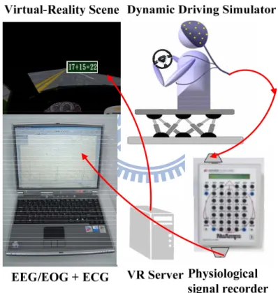
The most concerned issue in dual-task studies was the effect of distraction on driving because it directly related to public safety. For example, using cell-phone, tuning radio or looking at the road-sign could distract the drivers from their driving task and cause serious traffic accidents. However, the driving experiments were very dangerous if they were took place on road. The environment was employed in the setup of dual-task experiment as shown in Fig. 2-1.
Fig. 2-1: The illustration of the experimental setup.
It includes the dynamic VR driving environment and the EEG-based physiological measurement system.
With combining the technology of virtual reality (VR), a driving environment was constructed for the safety of driving experiments in our lab. In this study, a VR-based driving system was applied for interactive driving experiment. VR
technology is gradually being recognized as a useful tool for the study and assessment of normal and abnormal brain function, as well as for cognitive rehabilitation [17]. It included three major parts as shown in (1) the 3D highway driving scene based on the virtual reality technology, (2) a real vehicle mounted on a 6-DOF motion platform, and (3) a physiological signal measurement system with 36-channel EEG/EOG/ECG sensors. The full details of experimental system architecture will be described as followers.
2.1 Dynamic Driving Environment
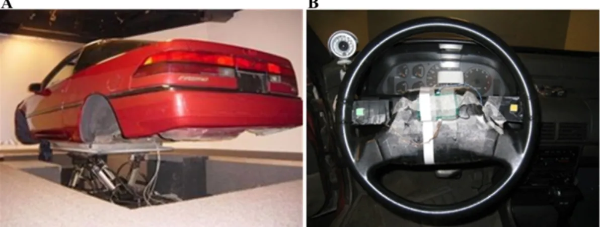
A virtual-reality (VR) based highway-driving environment was used to investigate the changes on drivers’ distraction effect. Some of our previous studies to investigate changes in drivers’ cognitive states during a long-term monotonous driving have also used the same VR-based environment [12] [17] [36]. The VR driving environment includes 3D surround scenes projected by seven projectors and a real car mounted on a 6-degree-of-freedom (as showed in Fig. 2-2(A)) Stewart platform to provide the kinesthetic stimuli [37]. During the driving experiments, all scenes move according to the displacement of the car and the subject’s maneuvering of the wheels (as showed in Fig. 2-2(B)) which make the subject feel like driving the car on a real road. The dynamic driving environment provided a safe, time saving and low cost approach to study human cognition under realistic driving events. The subjects could interact directly with the environment and receive the most realistic driving conditions during the experiments.
Fig. 2-2: Pictures showed the dynamic VR driving environment.
This equipment is in the Brain Research Center of National Chiao Tung University, Taiwan, and ROC. (A) One real car in the 3D VR environment was mounted on the 6-DOF motion platform. (B) The steering wheel of this car was used to handle the car and the subjects interacted directly with VR-environment through this steering wheel. There were two buttons (yellow and green) on the steering wheel for subjects to answer the mathematic equations. A camera was places at the left part of the steering wheel to monitor each subject during the experiment.
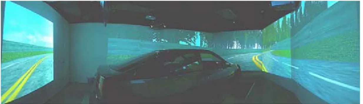
The VR scene was generated by the Virtual-Reality technology with a World Tool Kit (WTK) library. The VR scenes of different viewpoints were projected on corresponding locations. Fig. 2-3 showed the layout of our simulator. The front screen marked 1 and 2 was overlapped by two polarized frames to reach the binocular parallax. The frames for the left and right eyes were projected onto the frontal screen with two projectors, respectively. By wearing special glasses with a polarized filter, the configuration provided a stereoscopic VR scene for a 3D visualization. In our VR scene, the surrounded screens covered 206° frontal FOV and 40° back FOV, as shown in Fig. 2-4. Frames projected from 7 projectors were connected side by side to construct a surrounded VR scene. The size of each screen had diagonal measuring 2.6-3.75 meters. The vehicle was placed at the center of the surrounded screens. Detailed information was shown in Table-1.
Fig. 2-3: The picture showed the configuration of the 3D surrounded scene.
The 3D VR scene consisted of 7 projectors, creating a surrounded view. The frontal screen was overlapped by 2 projector frames in different polarizations, providing a stereoscopic VR scene for 3D visualization.
Fig. 2-4: The picture showed the overview of surrounded VR scene.
The VR-based four-lane highway scenes were projected into surround screen by seven projectors.
2.2 Experimental Design
To investigate the effect of stimulus onset asynchrony (SOA) on the behavioral performance and differences on brain activities between single- and dual- task conditions in a virtual environment, we designed two tasks: unexpected car deviation and calculation of mathematical equations. The combinations of these two tasks provided different distraction effects to the subjects.
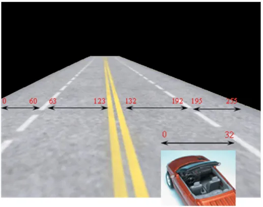
We developed a VR highway environment with a monotonic scene and eliminated all unnecessary visual stimuli as shown in Fig. 2-5. The four lanes from left to right were separated by a median strip in the VR-based scene. Our design was that the car must be kept in the third lane form the most left. The distance from the left side to the right side of the road was equally divided for outputting digital signal from WTK program, and the width of each lane and the car was 61 units and 32 units, respectively (as showed in Fig. 2-5). In the VR scene, the simulated driving speed was controlled by a scheduled program, thus subjects need not to step on paddles, to prevent large muscle activity on the throttle or brake.
Table-1: The Specification of driving simulator
Screen Number or Location Dimension
Screen Number 1, 2, 3, 4 (FOV 42°) (W)×(H) = (300 cm)×(225 cm)
Screen Number 5, 6 (FOV 40°) (W)×(H) = (270 cm)×(202 cm)
Screen Number 7 (FOV 40°) (W)×(H) = (210 cm)×(157 cm)
Vehicle Dimension (L)×(W)x(H) =
(430 cm)×(155 cm)×(140 cm)
Driver to Front Screen (1, 2) 370 cm
Driver to Left and Right Screen (5, 6) 220 cm (Left) and 300 cm (Right)
Fig. 2-5: The illustration of the monotonic high way scene.
The monotonous scene was designed to reduce the visual disturbance. The width of highway from the left to right side was equally divided into 256 units and the width of the car was 32 units.
We designed four sessions in one complete driving simulation experiment for each subject and the session duration was 15 minutes. In each session, the subject sat in front of the monitor with their hands on the steering wheel to control the car in the center of the third lane (from the most left lane). Among these four-session experiments, the subjects were forced to rest for ten minutes between every two sessions to avoid getting tried. On the other hand, to avoid anticipative effect for subjects the events were presented to the subjects randomly [38], as shown in Fig. 2-6. The inter-trial intervals were set from 6 to 8 seconds and the independent trials were not interaction to affect the subject. Thus a total of 100 trials could be presented to the subject in each session to ensure the number of events is enough for statistical analysis. There were about 80 trials in each case during one entire experiment.
Fig. 2-6: The illustration of the experimental paradigm.
Five cases were randomly appeared and the inter-trial intervals were varied from six to eight seconds. There were four sessions (15 minutes / per session) in each experiment.
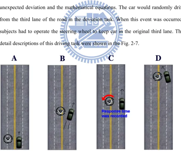
Since the main purpose of this experiment was to investigate the distraction effect in dual-task conditions. Therefore, two tasks were designed including the car unexpected deviation and the mathematical equations. The car would randomly drift from the third lane of the road in the deviation task. When this event was occurred, subjects had to operate the steering wheel to keep car in the original third lane. The detail descriptions of this driving task were shown in the Fig. 2-7.
Response time was recorded
A
B
C
D
Response time was recorded Response time was recorded Response time was recorded Response time was recordedA
B
C
D
Fig. 2-7: The illustration of the deviation event.
There are four steps in one complete deviation event. (A) Vehicle moving in straight line; (B) the onset of deviation event; (C) response to the deviation and (D) vehicle back to middle lane.
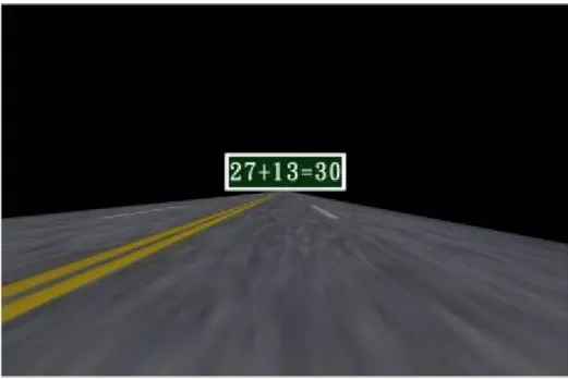
Two-digit addition equations were presented to the subjects in the mathematics task as shown in Fig. 2-8. The answers to the equations were already designed to present with the equations but they could be either right or wrong. The subjects were asked to press the buttons on the steering wheel as soon as they can. When the equation is correct, the subjects must press the right button. On the other hand, they would press the left button for the wrong mathematic equation. The event allotment ratios were 50% and 50% for right and wrong equations, respectively.
Fig. 2-8: The illustration of the mathematic equation.
The mathematic equation would be showed in front of the windscreen and the subjects were asked to response the answer. If the equation was correct, the right button on the steering wheel (as showed in Fig. 2.2(B)) might be pressed. On the other hand, the subject might press the left button when the equation was wrong.
The combinations of these two tasks were used to provide different distraction effect to the subjects. Five conditions were developed to study the interaction of the two tasks, they are: (A) math was presented at 400ms before deviation (math-400ms-deviaiton), (B) two tasks were presented at the same time
(deviation-400ms-math), (D) only math presented (single-math) and (E) only deviation occurred (single-deviation). The illustrations of the five conditions were shown in Fig. 2-9. A pilot study was designed to determine the time of stimulus onset asynchrony, and the result suggested the interaction between tasks is significant with 400ms time interval. Thus, we adopted 400 ms as the time of stimulus onset asynchrony.
Fig. 2-9: The illustration of five cases in our experiment.
The 5 cases were randomly appeared in the whole experiment. Each sub-figure shows the relationship between the deviation onset and math occurred. M is the mathematic equation and D is the task of car deviation. (A) Case 1: math was presented at 400ms before the deviation onset. (B) Case 2: math and deviation occurred at the same time. (C) Case 3: math presented at 400ms after the deviation onset. (D) Case 4: only math presented. (E) Case 5: only deviation occurred.
2.3 EEG Signal Acquisition
A standard for the placement of EEG electrodes proposed by Jasper in 1958, which is known as the 10-20 International System of Electrode Placement [39] is used in the electrode cap. An illustration of the 10-20 system is shown in Fig. 2-9(A), the electrodes are named according to the location of an electrode and the underlying area of cerebral cortex. An electrode cap was mounted on the subject’s head for signal acquisition as shown in Fig. 2-9(B).
The letters F, C, T, P, and O were refer to the frontal, central, temporal, parietal, and occipital cortical regions on the scalp, respectively. The term “10-20” means 10% and 20% of the total distance between specified skull locations. The percentage-based system allowed differences in skull locations. The physiological data acquisition used 30 sintered Ag/AgCl EEG/EOG electrodes with a unipolar reference at right earlobe and 2 ECG channels in bipolar connection placed on the chest.
The 36 electrodes including 34 EEG/EOG channels , 2 ECG channels (bipolar connections between the right clavicle and left rib), and one 8-bit digital signal produced form VR scene were simultaneously recorded by the Scan NuAmps Express system (Compumedics Ltd., VIC, Australia) shown in Fig. 2-10. It was a high-quality 40-channel digital EEG amplifier capable of 32-bit precision sampled at 1000 Hz. Table-2 showed the specifications of the NuAmps amplifier. Before acquiring EEG data, the contact impedance between EEG electrodes and skin was calibrated to be less than 5kΩ by injecting NaCl based conductive gel. The EEG data were recorded with 16-bit quantization levels at a sampling rate of 500 Hz in this study. All EEG data were preprocessed using a low-pass filter with a cut-off frequency of 50 Hz in order to remove the power line noise and other high-frequency noise. Similarly, a
drifts.
Fig. 2-10: The EEG apparatus.
This figure showed the EEG apparatus of the physiological recording. A: the 30 channel location. The letters used are: F: Frontal lobe. T: Temporal lobe. C: Central lobe. P: Parietal lobe. O: Occipital lobe. Z: refer to an electrode placed on the mid-line. B: The NuAmps EEG amplifier and the electrode cap.
2.4 Subjects
We have used a set of 11 subjects to collect EEG data for the investigation and the participants were the same as used in [17]. The subjects’ ages range between 20 to 28 years old, with a mean of 24 years. They were requested not to drink tea, smoke, drink caffeine, use drugs, or drink alcohol, all of which could influence the central and autonomic nervous system, for a week prior to the main experiment. The subjects had to pay attention to the designed conditions and respond as quickly as they can. We
Table-2: Specifications of NuAmps
Analog inputs 40 unipolar (bipolar derivations can be computed)
Sampling frequencies 125, 250, 500, 1000 Hz per channel
Input Range ±130mV
Input Impedance Not less than 80 MOhm
arranged the experiment in the morning and asked each subject to wash their hair right before coming for experiment so that we can collect more useful data. Before the beginning of each experiment, the subject needed a 15~30 minutes practice depending on when they got used to perform designed two tasks. Each subject had to achieve 4 sessions (15 minutes per session) and took a break between sessions. So a complete experiment took about one and a half hours to complete.
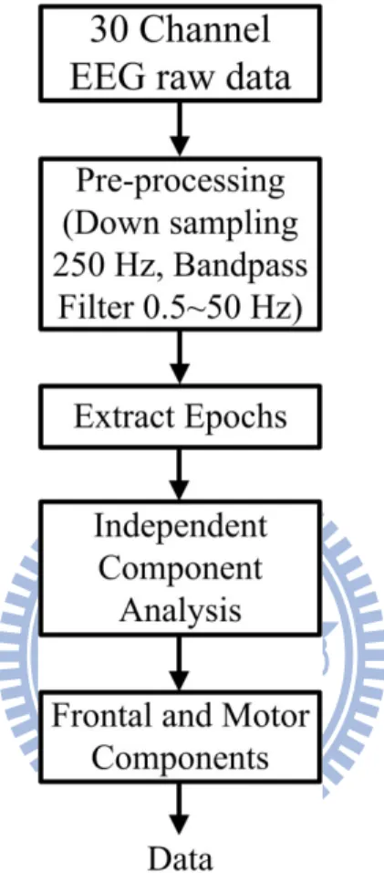
3. Methods
After the recording of the multi-channel EEG signals from 11 subjects, the data were analyzed for the study of distraction effect. EEG epochs were extracted from the recorded EEG signals after sown sampling, filter and artifact removal. We used Independent Component Analysis (ICA) [40] to separate independent brain sources. After the recorded EEG data analysis, we choose the data in Frontal and Motor components to be our feature for investigating the distraction levels. The extracted feature about EEG power must be processed first to be compatible with SOM. The steps of processing included downsizing the dimension, removing the baseline, reducing the variation among all subjects, normalizing and smoothing. The data have been adequately represented in the input space, and SOM training was performed. The algorithm of SOM was first demonstrated in an abstract system, without reference to any biological structures or signal types. Then we defined a mapping from the input data space R500 onto a two-dimensional array of neurons. We chose a rectangle lattice
with dimensions 25×25 and two phases learning process [27]. In this study, we proposed two methods to recognize the EEG epochs which were not trained the maps. The data base was created by the some taught maps and used the data set for the recognition of new EEG epochs from new or the same subjects.
3.1 EEG Signal Processing
Fig. 3-1 showed the flowchart of the proposed data analysis procedure for EEG signals. The EEG data were recorded with 16-bit quantization level at a sampling rate of 500 Hz and the recording were down-sampled to sampling rate equaled 250 Hz for the simplicity of data processing. The EEG data were then processed using a simple
low-pass filter with a cut-off frequency of 50 Hz to remove the line noise (60 Hz and its harmonic) and other high-frequency noise for further analysis. A simple high-pass filter with a cut-off frequency of 0.5 Hz was used to remove the DC drift.
Fig. 3-1: The flowchart showed the EEG signal processes.
The EEG raw data were pre-processing by this flowchart. At the beginning, we used low-pass filter and high-pass filter to remove the line noise and the DC draft. All epochs in the same case were extracted from the continuous EEG data and run the ICA. After running ICA, the source segregation of each subject was extracted.
Since we had designed different cases with the combinations of the driving and the mathematic tasks, thus the EEG response related to different cases should be extracted from the original EEG signals for further analysis. We extracted epochs from continuous EEG data and combine all epochs to run Independent Component
data equals to the length of a case. The ICA methods were extensively applied to solve the problem of EEG source separation, identification, and localization since 1990s [41-46]. We used the method of ICA to separate independent brain sources. The activation in Frontal areas was induced by mental task which were reported in the previous studies [17, 18]. The studies also showed that the spectra in Motor component were difference between the single- and dual- task conditions. We extracted the processed EEG signal in Frontal and Motor components to be our features for investigation the distraction levels by SOM in this study.
3.2 Features Extraction
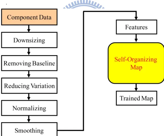
The features were the EEG data in Frontal and Motor component. Before we analyzed the extracted component data by SOM, the feature had to be processed. We wanted the features clearer and less variation. The flowchart of features processing was showed in the Fig. 3-2. We proposed some methods to process our extracted data. The detail steps and meaning of each method would be described in detail.
Downsizing
We designed the stimulus onset asynchrony (SOA) experiment, especially the different time interval of the dual tasks. The extracted features were the epoch-based. There was huge amount of information in our original EEG data. The data were epoch-based and included the information of timing. There were five thousand time points (1 second is the baseline and the other 4 seconds is phasic) in one epoch. In this research, the feature with combined with the EEG signals in Frontal and Motor
components to provide the more clear phenomenon than the data in each single component. Although the time points of EEG epochs in the two components equaled to five seconds, the dimensions of combined features were twice than the original EEG epochs in single component. We wanted to reduce the dimensions of the combined features and not lose any information about time and the perturbation of frequencies in each epoch. We could see the Fig. 3-3 to understand the detail information. Each epoch was equally divided into ten intervals. The length of phasic part in each epoch was 4 seconds so one interval was 400 milliseconds. We applied Fast Fourier Transform (FFT) for each interval to transform the signal from time domain to frequency domain.
.
Fig. 3-2: The flowchart of steps about EEG data processing and analyzing.
The two parts are feature processing and then using the processed data to train the maps by SOM algorithm. We applied these steps to process the EEG signals (as showed in the left part of this figure). Then the power spectra were the input data for
After applying the FFT, The main difference in power spectra among five cases could be observed about 5~14 Hz in Fontal component and 8~25 Hz in Motor component [17]. But there were 50 frequencies for each time point in the original EEG epoch. To reduce the dimensions of each interval, these values in the active bands by dealing with tasks were reserved. We just preserved the 1~20 Hz of Frontal component and 1~30Hz of Motor component in each interval. Then the data for Frontal (Motor) component in each interval were 20 (30) Hz and there were 10 intervals in each epoch. The features of Frontal or Motor components were reduced from 4000 time dimensions to 200 or 300 frequency and time dimensions, respectively. After this step, we got fewer dimensions and preserved the timing and frequency information in each interval.
Removing Baseline
There were four designed sessions in one complete experiment and the EEG signal was collected during one hour. There were many epochs in each session, and Fig. 3-3: The figure showed ten intervals and the baseline.
The length of each epoch from event-onset to event-offset during the experiment was 4000 milliseconds (4 seconds). One trial was divided to ten intervals so the length of all intervals was 400 milliseconds. The frequencies less than 20 (30) Hz in Frontal (Motor) component were reserved in this step. There were 50 points in each intervals and one epoch would be reduced to 500 points.
the events were presented to the subjects randomly in order to prevent anticipative [38]. Since we had designed different cases with the combination of the driving and the mathematic tasks, thus the EEG response related to different cases should be extracted from the analyzed EEG signals. To investigate the changing on brain activities between single- and dual- task conditions in a virtual environment, we just analyzed the EEG signals from onset of the event to the end of that epoch. The baseline was the mean of the EEG signal one second before the event onset. In order to investigate the changes in spectral power and the perturbations in the oscillatory dynamics of ongoing EEG, the baseline of each EEG epoch was removed by a dividing method. The unit of EEG signal is decibel (dB), and the dB is a logarithmic unit of measurement that expresses the magnitude of a physical quantity relative to a specified or implied reference level.
Because the FFT was applied to all EEG epochs, there were 50 frequency points originally. However, after the step of downsizing was processed, there were just 20/30 frequency points (1~20Hz/1~30Hz) for Frontal/Motor component. The length of baseline was 1000 milliseconds in Fig. 3-3. In other words, there were 1000 time points and 20 or 30 frequency points in each time point. The baseline was averaging all same frequencies which located at this time interval. Because dB is a logarithmic unit, each particular frequency in the EEG epoch was divided by that frequency during the baseline. After this step, we can ensure the EEG signals were main caused by the responding the tasks, excluded of reasons by the “state of mind”.
There were four sessions in one complete experiment. Each session of all experiments was set in the same circumstance, and the subjects were asked to keep the same psychological and physical situation during the experiment. However different people might not have the same phenomena for the same task; in other words,
among people. We wanted to analysis the influence of distraction instead of the difference among all subjects. In order to decrease the diversity in people and keep the variation among all five cases, we proposed this method of subtracting mean vector.
Reducing Variation
All epochs of five cases in the same subject were extracted from the data set. There were five hundred points in each epoch which was contained two hundred points from Frontal component and three hundred points from Motor component. Each dimension of all epoch extracted before from case 1 to case 5 was averaged to get one mean value. There was one mean number for one dimension from these extracted EEG epochs. We called this vector mean vector. The dimensions of mean vector and processed EEG signals were the same. The method of computing was showed in Fig. 3-4.
We subtracted this mean vector from each EEG epochs in that subject. If this step Fig. 3-4: The method of calculating the mean vector.
All EEG epochs of five conditions in the same subject were extracted from the data set. The mean value would be calculated for each dimension of these epochs by averaging all number in the current dimension. There were five hundred dimensions in each epoch and we would get the same numbers of mean value. These mean values were called mean vector.
of subtracting mean vector was not performed, the variation among subjects would be presented by the SOM map. In practice, the performance of the maps with subtracting the mean vector would be better. We would discuss this issue into details in Section 5-1.
Normalizing
Although we subtracted the mean vector for all epochs in each subject, the variation among the trials was still in our data. For example, someone performed two tasks A and B. However these two tasks were in the same condition, they were not happened in sequence. Many events in other condition would be appeared during the interval between A and B. by reason of events random occurred, the level of excited for these two tasks might be different. Before running the Self-Organizing Map with the multiple high dimension data, it is important to reduce the variation among different epochs. We carried out a normalization method like Z-Score to remove this abnormality. This algorithm was applied for each particular case by the order number of subjects. There were n trials in each case of one subject. First the mean value (Smean)
of those trials was computed by the following equation (1):
(1)
Where X is the input space, n is the total number of epochs in each case, i is the index of epoch number, and d is the dimensions of the input space.
In the second step the standard deviation (Sstd) was calculated by the same data by the
following equation (2):
∑ ∑
∑ ∑
= = = ==
n i feature d n i feature d meand
i
X
S
1 1 1 11
)
,
(
. (2)
Then we took these two values to normalize all epochs in that case. Each frequency in every trial was subtracted by the mean value (Smean) and divided by the standard
deviation (Sstd). The normalization of trial T was processed by the following equation
(3):
. (3)
Smoothing
We used a componentwise moving average to smooth the power spectra data. The size of moving window was the 10% epochs of that case in that subject, and the window was shifted by 1 epoch. The moving was processed by circular motion. For example, there were 100 EEG epochs in that case. The first window used epochs 1 through 10, the second window used epochs 2 to 11, and the latest window was used epochs 100 through 9. A moving average (computed using the 10% epochs) was used to minimize the presence of artifacts in the EEG signals of all epochs in that case. Thus for each case and subject, EEG signals in Frontal and Motor were well enough to be input data for the SOM model.
3.3 Computation of Self-Organization Maps
Self-Organizing Maps (SOM) offer an approach to brain activities that provides a
∑ ∑
∑ ∑
= = = =−
=
n i feature d n i feature d mean stdS
d
i
X
S
1 1 2 1 11
)
)
,
(
(
std mean feature dS
S
d
i
X
d
i
X
=
−
=)
,
(
)
,
(
~ 1mechanism for visualizing the complex distribution of cognitive states. The maps is defined by k neurons (locations) arranged as 1-, 2-, or 3-D lattice and easily realized that the topographic organization of the data. Increasing the number of locations k increases the accuracy of the results of labeling. Each neuron in the map contains an
n-dimensional (same as the input data) reference vector during the unsupervised
learning (training) process. When the unsupervised training process is over, the topographic organization of the map will adequately represent the input space. Thus, similar inputs will project near each other onto the near neurons in the map. Then the map will construct a structure by the input data. Topological neighborhoods can be of different shapes such as rectangle or hexagonal. In this research, we chose k = 625 (a rectangle lattice with dimensions 25 and 25). The maps were initialized, taught, and evaluated by SOM toolbox for MATLAB [47].
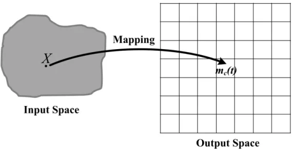
The initial step in the SOM routine is to define a random distribution of neurons, and there is one reference vector in each neuron in this map. All reference vectors mi
(i=1~k) must have random initial value and equal the dimension in the input space. Each neuron in the map will have a reference vector of 500 coefficients. In Fig. 3-5, for each input vector x(t), a reference vector mc(t) with minimum Euclidean distance
from the input is searched for by the following equation (4):
(4) The input data does not become part of a group at this time; it is simply used to adjust the location of the SOM node in the input space.
In Fig.3-6, the best-matching model vector mc and the model vectors mi in its circular
neighborhood are then modified toward the value of the input vector by the following equation (5):
(5) The magnitude of the learning coefficient α(t) decreases monotonically. Also the
size of the neighborhood of mc decrease at successive inputs. At the beginning of the
self-organizing its neighborhood on the map is wide, while at the end only the nearest neighbors of mc(t) are modified. The learning consisted of two phases. In the first
phase, the learning coefficient α(t) decreased from 1 to 0 in 75000 steps, while the
radius of the neighborhood decreased from 25 to 1. In the second phase, α(t)
decreased from 0.1 to 0 in 50000 steps, while the neighborhood radius decreased from 6 to 1. In both phases, the samples were presented randomly.
Fig. 3-5: The properties of the map
The X in the input data was mapping onto the map. The Euclidean distance from X to mc(t) was the minimum.
By the end of the training phase, this map may be useful until each neuron in the map is labeled. In ordered to label all neurons in the map, the input data was pre-classified into designated categories. There is a model vector in each neuron, and the Euclidean distance would be computed to each labeled patterns. The pattern would be located in that neuron with smallest distance then became the best stimulus for that neuron. This procedure closely resembles the way sites in the brain get labeled by stimulus features that maximally excite neurons at that time. Such a labeling procedure was applied to all the neurons in the map. Then we can run the voting scheme. Each neuron will be finally assigned a label that corresponds to the species whose patterns elicited a maximal response with the highest frequency. In other words, there may be several patterns in one neuron after the step of locating. For example, 9 patterns were in the same neuron (case-1:1, case-2:0, case-3:1, case-4:7, case-5:1), and the neuron would be assigned as ‘case-4’. The reason was that the Fig. 3-6: The illustration of the neighborhood size
The reference vectors in the best-matching neuron and its neighbor neurons would be adaptive to fit that input vector. (A) The neighborhood function in this study was used the Gaussian function. (B) The coverage of different neighborhood size.
neuron, we would not label that neuron. The method of labeling would eventually produce a well ordered partition of the map such that groups or clusters of neurons will respond maximally to the same class of patterns. Such a topographic map creates similarity relationships and can be used for pattern classification.
The maps were trained by the description as the above. The structure of the trained maps represented the phenomenon of all EEG epochs in each case. There were still some unlabeled neurons in the middle of each main area. We set a reference vector for each neuron during the steps of training and each reference vector would be adapted during the learning phase. The neighborhood size was reducing by the steps of training, and the neurons in the area of influence would get the chance of adapting. The structure of all maps was more consistent with the input data during this learning mechanism. Although there were no any data in these unlabeled neurons, there was a reference vector in the unlabeled neuron to represent the phenomenon and it must be similar to the reference vector or EEG epochs which located on the neighbor neurons. By this learning theorem, we marked each unlabeled neuron. If there was an unlabeled neuron in the middle of an array like Fig. 3-7, the distance (Euclidean distance) to each neighbor neuron would be computed. We could find the minimum distance between the two neurons, and then that unlabeled neuron would be labeled. The label of these two close neurons must the same. After applying this step, there were no unlabeled neurons in the trained maps and the better maps would be generated. We could create a data base to recognize the EEG signals of distraction effects.
3.4 Recognizing EEG through SOM
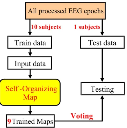
SOM was applied not only for training the maps but also testing the data by trained maps. We designed two methods to verify the testing data by these trained maps. The difference between these two methods was the training data. In the first model, the half EEG epochs from each subject were the training data. On the other hand, we chose all EEG epochs from one subject to be the training data in the second method.
The first method was cutting all EEG epochs into 2 parts and those EEG epochs were processed as description before. The separation was based on the subjects. The half of the data in one subject was partitioned into the training data and the other EEG epochs were the testing data. We used the training data to get the maps by SOM with the same parameters. All unlabeled neuron in the maps would be made up first. The reason was the EEG epochs in the testing data might not always stimulate labeled neurons. In other words, A EEG epoch might have the minimum distance to an Fig. 3-7: The enhancement of labeling.
The method of labeling the unlabeled neurons. (A) The grey neuron in the middle of this array is the unlabeled neuron. This unlabeled neuron neighbors two labeled neurons (blue and res). (B) We compute the Euclidean distance from the unlabeled neuron to all neighborhood neurons and find the minimum value. The label of that unlabeled neuron equals to the neighborhood neuron with the minimum distance.
making up the map, the testing data could be verifying this trained map. The flowchart about the first method about training and testing was showed in Fig. 3-8.
The other simulation was in the second method. There were still training data and testing data. All EEG epochs were processed by the steps showed in Fig. 3-1 in order to remove the variation and difference between subjects and trials. Then we chose the EEG epochs in one subject to be the testing data and the other was the training data. Nine maps were generated by the same parameters as before setting. The unlabeled neurons in these nine maps would be labeled first to provide complete information about relations among neighborhood. Then a data base was created by Fig. 3-8: The flowchart about first method of train and test.
All epochs were processed first and then separated into two parts. The half of epochs was the training data and the other half epochs the testing data. The parameters of SOM were the same as before.
these nine filled maps and we applied it to verify the testing data. Each epoch of testing data located on one neuron of each map in this data base and could be estimated case which was this epoch was belonged. We got nine results by the data base and classified the EEG epoch by voting. The class with maximal frequency was assigned to that EEG epoch. Fig 3.9 showed the flowchart about the second method of train and test.
Fig. 3-9: The flowchart about second method of train and test.
All epochs were processed first and then the EEG epochs of one subject were chose to be the testing data. 9 maps were trained by the other epochs and the parameters about SOM were the same as the first method of train and test. A data base was created by these nine trained maps and we applied it to classify all EEG epochs in testing data by voting.
4. Results
The main difference of brain activities among the five designed conditions was observed by the EEG analysis. The EEG signals in Frontal and Motor components which were collected from 11 subjects were the features for this study. We extracted EEG epochs in these two components to be the feature of distracted. Before running SOM algorithm, the features must be processed to reduce the variation. All processed EEG epochs were the input data into the Self-Organizing Map (SOM). The artificial neural network was used for the study of distraction. After training, the topological structure of input data was presented by the SOM to determine which neuron exemplified that particular distracted state. For each runs of SOM, a visual inspection was performed. Then, this agglomerative and partitive clustering algorithm was applied.
We characterize the phenomenon of components in the first section and compare processed features with the original features in the next section. The maps are trained by the processed features so the results of maps and analysis these maps are showed in the third section, including labeling, distributions of each subject’s EEG epochs, and the relation among neurons. Finally the results of recognition through two different models are shown in the latest section. Our results showed that the adaptive SOM process, in general way, may explain the organizations found in various brain structures.
4.1 Behavior and EEG Results
response time to deviation for dual tasks (case-1, case-2, and case-3) were significantly shorter than that for the single task (case-5). But there were no significant difference among the three dual-task conditions. The normalized response time to math was given in Fig. 4-1(B). The response time to math presented for dual tasks (case-1, case-2, and case-3) were significantly longer than that for the single task (case-4). But the normalized response times to math question and deviation for dual tasks were no statistical significantly difference.
Fig. 4-1: Bar charts of normalized response time.
These figures presented the normalized response time to the deviation (A) and mathematic equations (B) among 5 cases across 11 subjects.
The spectra in Frontal component were difference between the single-deviation and the dual-task cases in 5~17 Hz band. The activation in Frontal areas was induced by mental task which were reported in the previous studies [17, 18]. The studies also showed that the spectra in Motor component were difference between the single- and dual- task conditions around 8~25 Hz band. We chose these two components as the dominant feature to verify the distraction levels during driving as shown in Fig. 4-2.
Fig. 4-2: The phenomenon of Frontal and Motor components.
We extracted the features form Frontal and Motor components. (A) The main activations among the five conditions in Frontal were from 2 to 15 Hz. (B) We could observe the decrease of power from 8 to 25 Hz in Motor component.
4.2 Processed Features
We extracted the component data and the EEG signals in these two components were combined to be the features for this study. In order to reduce the variation and difference among all subjects, we proposed the processing methods for our extracted EEG epochs (as showed in Fig. 3-2). Fig. 4-3 shows the features without processing. The features just applied the method of downsizing so the dimensions of each EEG epochs equal 500. We can see that the value of power is not same strong among all subjects. Then we applied all methods showed in Fig, 3-2 to process the extracted EEG epochs. Fig. 4-4 shows the processed features. There is less variation in the processed features showed and the data is the input for the Self-Organizing Maps in this study.
Fig. 4-3: The features without processing.
The data showed in this figure is just reducing the dimensions. There is still some difference among all 11 subjects and 5 designed conditions.
4.3 SOM Results
4.3.1 Maps
Depending upon the random initialization, different features will settle in different parts of the 25*25 plane. However, the topological relations should be preserved in each trained map. We choose the EEG epochs of 4 cases (case-1, case-3, case-4, and case-5) to train the maps. The reason is that the effect of distraction is highest when two things were happened at the same time. In Fig. 4-5(A), there are 4 main clusters in this trained map with 2 phase training. We know that the EEG epoch of 4 cases are clearly recognized by the trained maps and there is some difference Fig. 4-4: The input data.
This was the inputs for the Self-Organizing Map. The input data was pre-processed by the steps described above.
when human response these 4 cases. The filled map by enhanced labeling is showed in Fig. 4-5(B). We can see 4 main clusters clearly in this filled map.
Fig. 4-5: Results of agglomerative clustering of EEG signals by SOM.
The map was trained by 4 cases. Four clusters mark by special colors are showed in the map. (A) The trained map by EEG epochs in 4 cases. (B) The filled map. The interaction of designed two tasks is indicated at the right part. M is the mathematic equation and D means the car deviation. In this map, the EEG epochs of case-2 (M and D are appeared at the same time) are not used.
In Fig. 4-6 we show maps. The investigations of SOM results allow concluding that SOM type algorithm can be used interpreting some mental tasks representing EEG data. We got many maps rapidly and the same phenomenon was found in these maps. We can find that some neurons which located in the middle of particular clusters are not labeled. The winning neurons are activity during training steps, and the neighborhood neurons are also adjusted. The connection among neurons is a key role in this algorithm. Competitive learning algorithm is competition among lateral neurons in a layer (via lateral interconnections) to provide selectivity (or localization) of the learning process. These unlabeled neurons are labeled by the close neighbor labeled neuron. After this computing, we get the better and clearer map in Fig. 4-7.
Fig. 4-6: Results of agglomerative clustering of EEG signals by SOM.
There are four maps in this figure. We verify the results by applying the algorithm many times. Five clusters mark by special colors are showed in each map. The interaction of designed two tasks is indicated at the right part. M is the mathematic equation and D means the car deviation. We combine these two tasks and stimulus onset asynchrony (SOA) to design five cases. The case-1~case-3 are the dual tasks and case-4~case-5 are the single tasks.
Our SOM based exploratory data analysis using EEG suggests existence of distinct signatures among these five cases. Fig. 4-6 and 4-7 show the topology relations of the collected EEG epochs. The EEG epochs of two single tasks are clustered well, but there are several subgroups to the dual tasks, especially the case-2. Although most neurons labeled case-2 are clustered to some main area, several special neurons are mixed together. The neurons labeled single conditions are mapped to the corners of each map and these two clusters are so congeries. The reason is the changing of brain signals for dealing with single task is consistent with each subject. When the mathematic question or car deviation appeared, the subject must response
them quickly and correctly. The brain resources are allocated to dealing with just one task during these two single conditions. But these two designed mental tasks are also combined to provide the dual-task situations in our experiment. Each subject is asked to response the tasks as soon as they can. When the subjects must do more than one task at the same time, these tasks scramble brain resources each other. Every subject doesn’t use the same strategy for responding dual-task condition. Someone answer the easy task first then deal with the complex task, but some people can deal with two tasks well.
Fig. 4-7: The filled map.
These four maps come from the maps showed in Fig. 4-1. Each unlabeled neuron in the map is marked a case by the method of flooding. Then all neurons represent one special case to show the topological relations. After flooding, these maps are clearer and easier to understand the distribution of EEG epochs among the five cases.
The three dual-task cases are clustered at the middle of the trained maps. The EEG epochs of case-1 and case-3 are grouped into two main areas, but we can see the
appeared at the same time. When these two tasks are appeared suddenly, subjects chose one tasks to respond first. By the different decision processes, the neurons labeled are close neurons labeled case-4 or labeled case-5. The two tasks are appeared with a 400ms interval and the subjects can have a short time to response one task well. In our maps, we can see the distribution of the cognitive state and investigate the distraction levels.
4.3.2 Labeling
We labeled all neurons by voting [31] [32] [48]. There might be several epochs from some cases in one neuron, because the phenomenon or characters of these epochs were too similar to recognize correctly. For every neuron, we counted the number of these epochs from every case. Then the neuron is labeled one case which has the maximum value by our calculating. The accuracy of each case is computable with this processing of voting. If the epochs are originally from the same case, these epochs are identified the right epochs. Otherwise the epochs do not come from the same case; they are mis-classified. In Fig. 4-8, the value in each neuron is the percentage of EEG epochs which are consistent with that neuron. When the value is less than 1, it means that the EEG epochs mapped into this neuron are more than 2 cases. We can call them mixed neurons.
Fig. 4-8: The frequency of each neuron.
There is one value in each neuron and this value is the percentage of EEG epochs which are consistent with this neuron.
We computed the accuracy of every case after labeling. The accuracy results of each trained map showed in Fig. 4-6 are in the Fig. 4-9. The accuracy of five cases is more than 90% in all trained map. Especially, the accuracy of case 4 and case 5 is even more than 95%. The accuracy of case2 in (C) is an exception and the hit rate is less 90%. But those mis-classified EEG epochs are still located in the neurons which are labeled case-1 or case-3. The epochs in three dual-task condition are easier to match the wrong neurons. In these steps of labeling, the average accuracy of five cases is about 90%. We can say that these maps in Fig. 4-4 are trained well and the
steps are enough to contract fully topology relation. We can classify the five cases well through the Self-Organizing Map, and the structure of the map is clearly to identify.
Fig. 4-9: The accuracy of each case.
The accuracy of each case was more than 90% in all four maps excepting case-2 in C. Especially the accuracy of case-4 and case-5 was near 100%. All EEG epochs were classified clearly by SOM in each time. The single-tasks are case-4 and case-5, but case-1 ~ case-3 are the dual-tasks considering the SOA.
4.3.3 The Distribution
The EEG signals were collected from 11 subjects. We applied many methods about feature processing to reduce the individual variation. Then the processed signals
were the input data and each epoch was mapped onto a 2-D array. It is an interesting and important thing to verify the location of all EEG epochs. We analyzed the distribution of all EEG epochs from different subjects to study the influence of distraction and human. The frequency of occurrence form across the SOM space was constructed by accumulating the number of EEG epochs mapped to each neuron. There were 2 numbers in each neuron: the first value is the order of each subject and the percentage was between the parentheses. We choose (A) map in Fig. 4-6 to analyze and draw the distribution of EEG epochs by different conditions and there are five cases in our experiment.
Case-1 is the dual-task condition. The mathematic questions appear before car deviation with a time interval of 400ms. The distribution of all EEG epochs from case-1 is showed in Fig. 4-10. The most data of case-1 is at the up part of the map but some special data are dispersive on this map.
Fig. 4-10: Distribution of EEG epochs in case-1.
The (A) map in Fig. 4-4 is verified the distribution of case-1. This figure shows the locations of all subjects and the percentage of all trials in each subject.
Fig. 4-11 shows the distribution of EEG epochs in case-2 and this array is match to (A) map in Fig. 4-6 and Fig. 4-7. It would seem that there are three or four sub-groups in this map. The car deviation and mathematic question are appearance at the same time to provide the most influenced effect during driving. The distribution of the EEG epochs in case-2 is dispersive. For example the EEG signals collected from subject 11 are located in these left, right, and down parts of this map. This phenomenon is consistent with the concurrence of brain resources.