利用多喇叭實現強健串音消除系統

國 立 交 通 大 學

電信工程學系

碩 士 論 文

利用多喇叭實現強健串音消除系統

Robust Crosstalk Cancellation for 3D Sound

Using Multiple Loudspeakers

研究生：蘇大中

指導教授：謝世福 博士

利用多喇叭實現強健串音消除系統

Robust Crosstalk Cancellation for 3D Sound

Using Multiple Loudspeakers

研究生 ：蘇大中 Student：D. J. Su

指導教授：謝世福 Advisor：S. F. Hsieh

國 立 交 通 大 學

電信工程學系碩士班

碩士論文

A Thesis

Submitted to Department of Communication Engineering College of Electrical and Computer Engineering

National Chiao Tung University in Partial Fulfillment of the Requirements

for the Degree of Master of Science

in

Electrical Engineering September, 2006

Hsinchu, Taiwan, Republic of China

利用多喇叭實現強健串音消除系統

學生：蘇大中 指導教授：謝世福

國立交通大學電信工程學系碩士班

摘要

傳統串音消除技術是針對一對喇叭來實現。而串音消除器主要的問題來自於 容易受到擾動的影響。由文獻可得知，當喇叭數增加則串音消除器消除串音的能 力亦隨之提升。同時，多喇叭架構對於擾動而造成雙耳音訊失真的效應較一對喇 叭要來得輕微。在本篇論文中，我們將呈現各種不同形態的串音消除器在三個喇 叭架構下，並且能夠達到節省成本及計算複雜度的目標。我們也會針對兩個喇叭 和三個喇叭架構的串音消除器作擾動分析，以及透過模擬數據來作為分析的依 據。

Robust Crosstalk Cancellation for

3D Sound Using Multiple

Loudspeakers

Student : D. J. Su Advisor : S. F. Hsieh

Department of Communication Engineering

National Chiao Tung University

Abstract

Traditional crosstalk cancellation is for two loudspeakers. The most critical

problem bothering us is the effect of perturbation. In several literatures, we know that

multiple loudspeakers arrangement results in good performance of crosstalk

cancellation. In addition, it is more robust for perturbation than two loudspeakers

setup. In this thesis, we show different types of crosstalk canceller of multiple

loudspeakers arrangement and economical realizations with less computational

complexity is achievable. Perturbation analysis is proposed in comparing two and

three loudspeakers setup. The simulation results are used to compare their

Acknowledgement

I would like to express my deepest gratitude to my advisor, Dr. S. F.

Hsieh, for his enthusiastic guidance and great patience, especially the

autonomy in research. I also appreciate my friends for their inspiration

and help. Finally, I would like to show my thanks to my parents for their

unceasing encouragement and love.

Contents

Chinese Abstract i

English Abstract ii

Acknowledgement iii

Contents iv

List of Tables vii

List of Figures ix

1 Introduction

...1

2 Transaural Stereo System

………4

2.1 Spatial Audio……….………..5

2.2 HRTFs……….6

2.3 Crosstalk cancellation………8.

2.3.1 Problem Formulation………9.

3 Crosstalk Cancellers

…...12

3.1 Conventional Two Loudspeakers Arrangement……...…….………13

3.2.1 Direct Forward Type………..…..………17

3.2.2 Least Square Forward Type………19

3.2.3 Shuffler Structure………20

3.2.4 A Simplified Shuffler Form.…..…………..………24

3.2.5 A Simplified Shuffler Form of Four Loudspeakers Arrangement…...28

3.2.6 Reduced-Order Modeling………31

4 Perturbation Analysis

…...…….………32

4.1 Perturbation Analysis for Filter Modeling..……….……….33

4.1.1 Analysis on Shuffler Form of Two Loudspeakers Setup...…………34

4.1.2 Analysis on Shuffler Form of Three Loudspeakers Arrangement...…38

4.1.3 Analysis on Simplified Shuffler Form…..………...44

4.2 Perturbation Analysis for Headmovement.…...………47

4.3 Optimum Loudspeakers Position for Robust Crosstalk Canceller…………50

4.3.1 Two Loudspeakers Arrangement………...……...…………52

4.3.2 Three Loudspeakers Arrangement………...………54

4.3.3 Four Loudspeakers Arrangement……….………56

4.4 Conclusions………59

5 Computer Simulations

……..………60

5.2 Two Loudspeakers Geometric………..……63

5.3 Three Loudspeakers Geometric………66

5.3.1 Least Square Forward Type………...……...………66

5.3.2 Shuffler Structure………...………..71

5.3.3 A Simplified Shuffler Form………...73

5.3.4 A Simplified Shuffler Form of Four Loudspeakers Arrangement…...78

5.4 Perturbation Analysis………82

5.4.1 Simulations on Filter Modeling………...……...……84

5.4.2 Simulations on Head movement………...……….91

6 Conclusions

……….……….95

List of Tables

5.1 The performance of shuffler form for two loudspeakers setup with different order

of FIR filters……...63

5.2 The CSF with different degree of freedom of the center loudspeaker………….65

5.3 The performance of least forward type crosstalk canceller for three loudspeakers

setup with different order of FIR filters………..66

5.4 The performance comparison of crosstalk cancellation by using least square

method for different numbers of loudspeakers arrangement………...67

5.5 The performance of shuffler form for three loudspeakers setup with different FIR

filter order………70

5.6 The performance of simplified shuffler form for three loudspeakers setup with

different orders of FIR filters………..…74

5.7 The performance of simplified shuffler form for four loudspeakers setup with

different orders of FIR filters………79

5.8 The error norm of equalization and crosstalk part for two loudspeakers shuffler

5.9 The performance of crosstalk cancellation for two loudspeakers shuffler form

after head movement………...91

5.10 The performance of crosstalk cancellation for three loudspeakers simplified

shuffler form after head movement………92

5.11 The performance of crosstalk cancellation for four loudspeakers simplified

List of Figures

2.1 The ITD and ILD………6

2.2 The setup of the dummy head………8

2.3 Signal and transfer function definitions for transaural stereo………10

3.1 Crosstalk cancellation system (Atal and Schroeder in 1963)………...13

3.2 Shuffler filter structure (Cooper and Bauck in 1989)………14

3.3 Geometry and transfer functions for three loudspeakers………..17

3.4 The structure of the direct forward type crosstalk canceller………18

3.5 The shuffler topology of three loudspeakers geometric (Cooper and Bauck in 1996)……….22

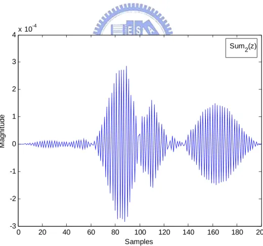
3.6 The impulse response of the filter ∑ ………22 ₂ 3.7 The impulse response of the filterC ………...23 ₂ 3.8 The impulse response of the filter ∆ ………23 ₂ 3.9 The simplified shuffler structure of crosstalk canceller for three loudspeakers arrangement………26

3.11 The impulse response of the filter∆ ………...27 ₃

3.12 Geometry and transfer functions for four loudspeakers………...28

3.13 The simplified shuffler structure of crosstalk canceller for four loudspeakers arrangement………30

4.1 The geometry of crosstalk cancellation system for multiple loudspeakers after filter modeling………..31

4.2 The factorized two loudspeakers shuffler form………33

4.3 The factorized three loudspeakers shuffler form………37

4.4 The factorized three loudspeakers simplified shuffler form………44

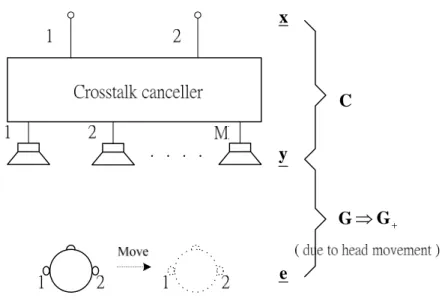
4.5 The geometry of crosstalk cancellation system for multiple loudspeakers due to head movement………46

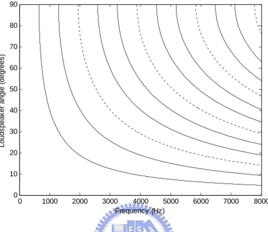
4.6 The condition numbers of G with different loudspeakers position………….51 ₂ 4.7 The condition numbers of G with different loudspeakers position………….53 ₃ 4.8 The robust bandwidth of different number of loudspeakers with the side loudspeakers located at ± °30 ………..56

5.1 The crosstalk cancellation results in frequency domain by using least square error method with loudspeaker located at ±30D………63

5.2 The crosstalk cancellation results in time domain by using least square method with loudspeaker located at ±30D………64

5.3 The crosstalk cancellation results in frequency domain of least square forward

type with the side loudspeakers located at ±30D and the center one located at

0D………66

5.4 The crosstalk cancellation results in time domain of least square forward type

with the side loudspeakers located at ±30D and the center one located at 0D...67 5.5 The signal power ratio R of different numbers of loudspeakers with different _c

filter orders………...68

5.6 The total errorε of different number of loudspeakers with different filter

orders………....68

5.7 The crosstalk cancellation results in frequency domain of shuffler structure with

the side loudspeakers located at ±30D and the center one located at 0D……...70 5.8 The crosstalk cancellation results in time domain of shuffler structure with the

side loudspeakers located at ±30D and the center one located at 0D………….71 5.9 The crosstalk cancellation results in frequency domain of simplified shuffler

form.………..74

5.10 The crosstalk cancellation results in time domain of simplified shuffler form…76

5.11 The CSF of different structure crosstalk canceller of three loudspeakers

arrangement………..76

arrangement………..77

5.13 The total error of different structure crosstalk canceller of three loudspeakers

arrangement………..77

5.14 The crosstalk cancellation results in frequency domain of simplified shuffler

form of four loudspeakers setup………...79

5.15 The crosstalk cancellation results in time domain of simplified shuffler form of

four loudspeakers setup………80

5.16 The signal power ratio after crosstalk cancellation R of two loudspeakers _c

shuffler form and three and four loudspeakers simplified shuffler form with

different FIR filter orders……….81

5.17 The total error of two loudspeakers shuffler form and three and four

loudspeakers simplified shuffler form with different FIR filter orders…………81

5.18 The crosstalk cancellation result in frequency domain after perturbing………..83

5.19 The crosstalk cancellation result in time domain after perturbing………...83

5.20 The norm of equalized error of two loudspeakers shuffler form with different

orders of IIR filter………86

5.21 The norm of crosstalk error of two loudspeakers shuffler form with different

orders of IIR filter………87

5.23 The crosstalk error of shuffler form versus direct forward type 2………...88

5.24 The equalized error of different structures of crosstalk canceller with different

IIR filter orders……….90

5.25 The crosstalk error of different structures of crosstalk canceller with different IIR

filter orders………...90

5.26 The signal power ratio R of crosstalk cancellation after head moving for _c

different numbers of loudspeakers………...94

5.27 The total error of crosstalk cancellation after head moving for different numbers

Chapter 1

Introduction

Using immersive audio techniques it is possible to render virtual sound sources in

3D space via a set of loudspeakers or headphones. The goal of such systems is to

reproduce the same sound pressure level at the listener’s eardrums that would be

present if a real sound source was placed in the location of the virtual sound source.

However, reproducing the 3D sound via two or more loudspeakers will suffer from

several factors to degrade the performances, such as room reverberance, crosstalk

disturbance and imperfection of the loudspeakers. In this thesis, we will focus on

crosstalk cancellation.

Previous work [13] has investigated that the design of conventional crosstalk

cancellation systems which deliver binaural audio to a listener has the serious

demonstrated that the performance of crosstalk canceller suffered from head

movement and have mathematically calculated the robustness of crosstalk

cancellation system. The approach proposed in [1] is to track the listener and adjust

the loudspeaker signals to maintain the binaural transmission so that a more robust

crosstalk canceller is possible. Recent work [9, 23] has demonstrated that if a number

of loudspeakers is used which exceeds the number of points in the listening space, the

performance of such a system can be improved. In such case, the reproduction is

sought and has better immunity of the head movement. Therefore, multi-channel

sound reproduction is our main focus in this thesis.

In this thesis, we will discuss how to synthesize the aural virtual reality

environment via multiple loudspeakers. We will focus on how to reduce the crosstalk

and design different types of crosstalk canceller so that the 3D sound can be

reproduced at listener’s ear precisely. Also, we will discuss how to factorize the

crosstalk canceller matrix so that economical realizations and less computation are

possible. In addition, we will discuss the robustness of crosstalk canceller by

perturbation analysis. The perturbation analysis of different structures of crosstalk

canceller for multiple loudspeakers arrangement is shown in chapter 4.

This thesis is organized as follows. In chapter 2, we will introduce the properties of

loudspeakers. Chapter 3 focuses on the design of crosstalk canceller using three

loudspeakers. Chapter 4 is the main part of this thesis; we will investigate the

robustness of crosstalk canceller and derive the optimum loudspeakers position for

different number of loudspeakers arrangement. In chapter 5, we will use computer

simulations to compare performances of different crosstalk cancellers and discuss the

robustness of crosstalk canceller. In chapter 6, we will make a conclusion to

Chapter 2

Transaural Stereo System

A transaural stereo system uses the binaural sound recording and reproduces them.

The system may have more than two loudspeakers. We will focus on the transaural

system with multiple loudspeakers. In this chapter, we will first introduce how the

human localize the sound source by the principle of ITD (interaural time differences)

and ILD (interaural level difference).

In section 2.2, we will illustrate how HRTFs (head-related transfer functions) can

aid in distinguishing sound location from one position to listener. Section 2.3 will

investigate the problems encountered in binaural reproduction via loudspeakers and

the idea of crosstalk canceller will be presented in detail. In the last section, we will

investigate the design of the transaueal stereo system and two types of layout

2.1 Spatial audio

The human hearing process is based on the analysis of input signals to the two ears

for differences in intensity, time of arrival, and directional filtering by the outer ear.

[11], [12] identified two basic mechanisms as being responsible for sound location

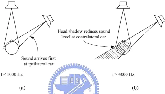
which are ITD (interaural time differences) and ILD (interaural level difference). As

described in [21], ITD and ILD cues that operated in different wavelength. For short

wavelengths (corresponding to frequencies in the range of about 4–20 kHz), the

listener’s head casts an acoustical shadow giving rise to a lower sound level at the ear

farthest from the sound source (ILD) as shown in Figure 2.1. (b). At long wavelengths

(corresponding to frequencies in the range of about 20 Hz–1 kHz), the head is very

small compared to the wavelength, and localization is based on perceived differences

in the time of arrival of sound at the two ears (ITD) as shown in Figure 2.1. (a). The

two mechanisms of interaural time and level differences formed the basis of what

became known as the duplex theory of sound localization. In the frequency range

between approximately 1 and 4 kHz, both of these mechanisms are active, which

results in several conflicting cues that tend to cause localization errors.

While time or intensity differences provide source direction information in the

horizontal plane, in the median plane, time differences are constant and localization is

head, torso, shoulders, and pinna, combined with resonances caused by the ear canal,

form the physical basis of the head-related transfer functions (HRTFs).

2.2 HRTFs

3D audio rendering systems are based on digital implementations of such

head-related transfer functions (HRTFs). In principle, it is possible to achieve

excellent reproduction of 3D sound fields using such methods, however, this requires

precise measurement of each listener’s individual HRTFs. In fact, the magnitude and

phase of these head-related transfer functions vary significantly not only for each

(a) (b)

Figure 2.1 The ITD and ILD. (a) In the low-frequency regime, sound is localized based on differences in the time of arrival at each ear. (b) At higher frequencies, sound localization is based on perceived level differences caused by head shadowing.

sound direction, but also from person to person. Current research [7] in this area is

focused on achieving good localization performance while using nonindividualized

HRTFs derived through averaging or modeling or based on the HRTFs of subjects that

have been determined to be “good localizer”. In [26], Begault found that there are

currently three major barriers in 3D audio implementations: 1) psychoacoustic errors

such as front-back reversals typical in headphone-based systems, 2) large amounts of

data required to represent measured HRTFs accurately, and 3) frequency and phase

response errors that arise from mismatches between nonindividualized and measured

HRTFs.

The HRTFs database we use is from MIT Multi-Media Lab in [27], each HRTFs

has 512 samples and with 44.1 kHz sample rate. The pickup of the HRTFs is a pair of

microphones embedded in the ears of a dummy head to simulate the ears of the

human head. The setup of the dummy head is shown in Figure 2.2. The spherical

space around the dummy head was sampled at elevations from -40 degrees (40

degrees below the horizontal plane) to +90 degrees (directly overhead). At each

elevation, a full 360 degrees of azimuth was sampled in equal sized increments. The

increment sizes were chosen to maintain approximately 5 degree great-circle

increments. In total, 710 different positions were sampled at elevations from -40

2.3 Crosstalk Cancellation

A simple way to reproduce the 3D sound is using headphones. Listening the

binaural signals via headphones can avoid the crosstalk interference, since the audio

signals are sent solely to their own destination. Because the listener would feel the

virtual sound image exists inside the head and be unable to provide sufficient realistic

perceptual feeling. Hence, using headphone for 3D sound might not be proper. To get

rid of the phenomenon, we would replace the headphones with two or more

loudspeakers.

In the case of conventional crosstalk canceller, this situation states playbacking the

binaural signals via a pair loudspeakers for one listener. However, the left ear of

listener received the sound not only from the left loudspeaker but also the right Figure 2.2 The setup of the dummy head.

loudspeaker and vice versa. This phenomenon is called crosstalk. These crosstalks

would disturb the directional perception in 3D sound reproduction since it would

change the spectrum, conveying the direction perception cues of the audio signals. In

order to eliminate the crosstalk, the crosstalk cancellation should be introduced.

2.3.1 Problem Formulation

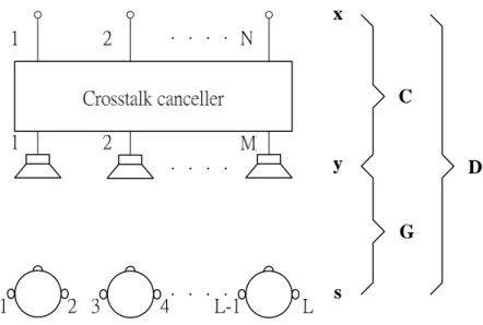
The algebraic structure of transaural stereo will be developed with the aid of Figure 2.3. In that figure, N program signals x x₁, ₂, ,x are to be used to create M _N

loudspeaker signals y y₁, ₂, ,y , which in turn result in L ear signals _M s s₁, ₂, ,s . _L

Let these three sets of signals be represented by the vectors

[

1 2

]

T N x x x = x (2.1)

[

1 2

]

T M y y y = y (2.2)

[

1 2

]

T L s s s = s (2.3)

where T denotes matrix transposition. Next, define three matrices of transfer functions. First let G be an L M× matrix, the acoustic matrix, such that element g is the _ij

transfer function to the ith ear from the jth speaker. Similarly, let C be an M×N

C D s y x G

crosstalk canceller from jth input to the ith output of the network, and let D be the

L N× matrix of desired transfer functions describing the overall transfer of signal

from the inputs of the crosstalk canceller to the ears, for which d is the transfer _ij

function to the ith ear from the jth crosstalk canceller input. With this notation in place,

the acoustic propagation can be written as the matrix form =

s Gy , (2.4)

the action of the crosstalk canceller can be written =

y Cx , (2.5)

and the desired transfer of signals is

=

s Dx. (2.6)

From these, a solution is found by solving

=

GC D (2.7)

for C. In this thesis, where N = 2, M = 2, 3, 4 and L = 2 so that G is a 2 M× matrix,

C is an M× and GC results in a 2 22 × desired transfer matrix D. In order to

deliver the binaural signals to listener precisely so that D must be an identity matrix. Thus, we will find the crosstalk canceller by solving G_{2 M×} C_{M 2×} =I_{2 2×} in chapter 3.

Chapter 3

Crosstalk cancellers

To achieve good reproduction of 3D audio it is necessary to precisely control the

acoustic signals at the listener’s ear. The simplest way to do this is to deliver binaural

signals through headphones. However, in many applications, e.g., home entertainment

environment, spatialized video-conferencing, it is preferable that the listener is not

required to wear headphones. If loudspeakers are used to deliver binaural signals, the

crosstalk signal that arrives at each ear from the other loudspeakers must be canceled.

This is achieved by pre-filtering binaural signals before send to loudspeakers and is

shown in Figure 3. 1.

In this chapter, we will discuss difference structures of crosstalk canceller of three

loudspeakers arrangement. In addition, economical realizations, less computations

1 h h2 h3 h4 1 g 2 g

3.1 Conventional Two Loudspeakers Arrangement

First, we consider the typical crosstalk canceller. Assume a symmetrical case here.

This case has two channels, two loudspeakers, and two ears, as shown in Figure 3.1. The acoustic transfer function matrix G

( )

Z is

( )

1

( )

_{( )}

2

_{( )}

( )

2 1 g z g z z g z g z ⎡ ⎤ = ⎢ ⎥ ⎣ ⎦ G . (3.1)

In order to reproduce the binaural signal at each ear, C

( )

z must be the inverse of the acoustic transfer function matrix G

( )

z , so that

( )

_{( )}

_{( )}

1

( )

_{( )}

2

_{( )}

( )

2 2 2 1 1 2 1 g z g z z g z g z g z g z − ⎡ ⎤ = _{⎢ ⎥} − − _{⎣ ⎦} C (3.2)

From Eq. (3.2), it requires four filters to realize crosstalk cancellation which has

heavy computation load. However, some simplification is possible in implementation. In 1989, Cooper and Bauck proposed shuffler structure which C

( )

z can be factored by the standard diagonalization technique of finding its eigenvectors and eigenvalues.

This results in the shuffler form.

( )

(

( )

( )

)

( )

( )

(

)

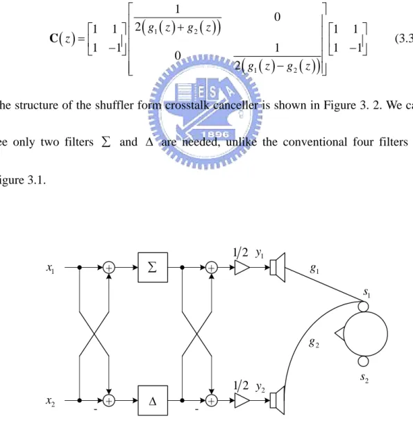
1 2 1 2 1 0 2 1 1 1 1 1 1 1 1 1 0 2 g z g z z g z g z ⎡ ⎤ ⎢ ₊ ⎥ ⎡ ⎤_{⎢ ⎥}⎡ ⎤ = ⎢ ₋ ⎥_{⎢ ⎥}⎢ ₋ ⎥ ⎣ ⎦_{⎢ ⎥}⎣ ⎦ − ⎢ ⎥ ⎣ ⎦ C (3.3)

The structure of the shuffler form crosstalk canceller is shown in Figure 3. 2. We can

see only two filters ∑ and Δ are needed, unlike the conventional four filters in

Figure 3.1. ∑ Δ 1 x 2 x 2 y 1 y 1 2 1 2 1 g 2 g 1 s 2 s

In our approach, we adopt the FIR filter and use the least square error method to

find out the finite impulse responses of the filters in Eq. (3.3). Let

( )

_{( )}

_{( )}

1 2 1 z g z g z ∑ = + (3.4) and

( )

_{( )}

_{( )}

1 2 1 z g z g z Δ = − (3.5)

then we can obtain two equation as follows:

( ) ( )

z g z1

( ) ( )

z g2 z d z1

( )

∑ ⋅ +∑ ⋅ = (3.6)

( ) ( )

z g z1

( ) ( )

z g2 z d2

( )

z

Δ ⋅ − Δ ⋅ = (3.7)

where d z₁

( )

and d₂

( )

z are the signal that we want to approximate . In the matrix form, these two equations can be expressed as follows:

⋅ = G c D (3.8) 1 2 0 0 ∑ Δ ⎡ ⎤⎡ ⎤ ⎡ ⎤ = ⎢ ⎥⎢ ⎥ ⎢ ⎥ ⎣ ⎦ ⎣ ⎦ ⎣ ⎦ 1 2 G d G d (3.9)

where G and ₁ G represent the convolution matrices of ₂ g n₁

[ ]

+g n₂

[ ]

and

[ ]

[ ]

1 2

g n −g n , respectively. The vector ∑=

{

∑

[ ] [ ]

0 ∑ 1 ∑

[

J−1

]

}

and

[ ] [ ]

[

]

{

Δ 0 Δ 1 Δ J 1

}

Δ = − represent the inverse FIR filters with J taps. The

desired response d_i =

{

d_i

[ ]

0 d_i

[ ]

1 d K_i

[

+ −J 2

]

}

=

{

1 0 0

}

for i =1, 2 represents the impulse response in time domain, where K is the number of taps of the

transfer functions.

K+J-2 such that the following square error as small as possible.

2 2

e = D G c− ⋅ (3.10) The least square error solution can be shown as

(

T

)

⋅ = T

G G c G D (3.11)

(

_T

)

−1 _T

=

c G G G D (3.12) Hence, the FIR filter would be

[ ] [ ]

[

]

{

c 0 c 1 c J 1

}

∑= − (3.13)

[ ] [

]

[

]

{

c J c J 1 c 2J 1

}

= Δ + − (3.14)

It should be mentioned that the desired signal can not be the pure impulse. It

requires an extra delay to decrease the least square error while approximating the

desired signal. The extra delay we choice is typically the half of the inverse FIR filter

order.

3.2 Three Loudspeakers Setup

Next, we look at the situation depicted in Figure 3.3, a symmetrical arrangement of

three loudspeakers and one listener. We have

( )

1

( )

_{( )}

3

( )

_{( )}

2

_{( )}

( )

2 3 1 g z g z g z z g z g z g z ⎡ ⎤ = ⎢ ⎥ ⎣ ⎦ G (3.15)

It should be mentioned that the solution of crosstalk canceller is not unique. Since

infinite number of solutions of C z_i

( )

. In the following sections, we will discuss some possible solutions of crosstalk canceller of three loudspeakers geometric and

illustrate how to find the crosstalk canceller.

1 g 2 g g3 × 3 2 C

3.2.1 Direct Forward Type

This structure has proposed by Cooper and Bauck in [10]. In order to reproduce the binaural signal at both ear accurately, the general solution is that C

( )

z must be the pseudoinverse of G

( )

z as shown below

( )

_H

( ) ( )

(

_H

( )

)

1

z z z z −

+ ₌

G G G G (3.16)

hence, the crosstalk canceller C

( )

z is

( )

z = +

( )

z

C G (3.17) Figure 3.3 Geometry and transfer functions for three loudspeakers.

( )

( )

( )

( )

( )

( )

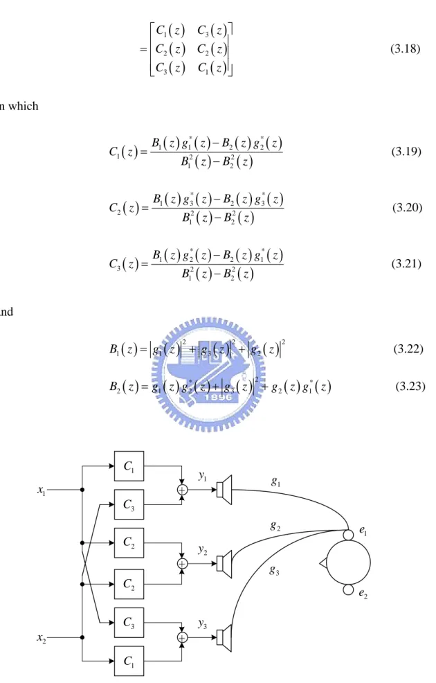
1 3 2 2 3 1 C z C z C z C z C z C z ⎡ ⎤ ⎢ ⎥ = ⎢ ⎥ ⎢ ⎥ ⎣ ⎦ (3.18) in which

( )

1

( ) ( )

1*

_{( )}

2

( ) ( )

_{( )}

*2 1 2 2 1 2 B z g z B z g z C z B z B z − = − (3.19)

( )

1

( ) ( )

3*

_{( )}

2

( ) ( )

_{( )}

*3 2 2 2 1 2 B z g z B z g z C z B z B z − = − (3.20)

( )

1

( ) ( )

*2

_{( )}

2

( ) ( )

_{( )}

1* 3 2 2 1 2 B z g z B z g z C z B z B z − = − (3.21) and

( )

( )

2

( )

2

( )

2 1 1 3 2 B z = g z + g z + g z (3.22)

( )

( ) ( )

_*

( )

2

( ) ( )

_* 2 1 2 3 2 1 B z =g z g z + g z +g z g z (3.23) . 1 y 2 y 3 y 1 x 2 x 1 e 2 e 1 g 2 g 3 g 1 C 1 C 2 C 2 C 3 C 3 C

The structure of the direct forward type crosstalk canceller is shown in Figure 3. 4. To perform these filters directly causes C z_i

( )

unstable due to the denominator of

( )

i

C z has non-minimum phase. Thus, in order to avoid the stability problem we can

find these filters by using the least square method

3.2.2 Least Square Forward Type

In order to overcome the problem of stability, we can find the crosstalk cancellation

filters by using the least square method. The structure of this type crosstalk canceller is same as Figure 3. 4. Our goal is that C

( )

z multiplied by G

( )

z equals an identity matrix I_{2 2×} with some extra delay. Since symmetric arrangement, the four equations need to solve become two equations as shown below

( ) ( )

( ) ( )

( ) ( )

( )

1 1 3 2 2 3 g z C z +g z C z +g z C z =d z (3.24)

( ) ( )

( ) ( )

( ) ( )

2 1 3 2 1 3 0 g z C z +g z C z +g z C z = (3.25)

In the matrix form:

= _s Gc D (3.26) 1 2 ⎡ ⎤ ⎡ ⎤_{⎢ ⎥ =}⎡ ⎤ ⎢ ⎥_{⎢ ⎥ ⎣ ⎦}⎢ ⎥ ⎣ _{⎦ ⎢ ⎥} ⎣ ⎦ 1 3 2 2 3 1 3 c G G G d c G G G 0 c (3.27)

where G₁, G₂ and G₃ represent the convolution matrices of g n₁

[ ]

, g n₂

[ ]

and

[ ]

3

The desired response d=

{

0 0 1 0

}

represents the impulse response

with K+J-1 taps and J 2 modeling delay in time domain. 0 represents the zero

vector with K+J-1 taps. Thus, the least square error solution can be obtained by Eq.

(3.11) and Eq. (3.12) then the FIR filter would be

[ ] [ ]

[

]

{

c 0 c 1 c J 1

}

= − 1 c (3.28)

[ ] [

]

[

]

{

c J c J 1 c 2J 1

}

= + − 2 c (3.29)

[ ] [

]

[

]

{

}

3 = c 2J c 2J +1 c 3J −1 c (3.30)

This type crosstalk canceller requires six FIR filters and causes complex calculation. In the next section, we will focus on factoring the crosstalk canceller matrix C

( )

z so that economical realizations are possible.

3.2.3 Shuffler Structure

This structure has proposed by Cooper and Bauck in [10]. Eq. (3.18) is useful in

showing that six filters are required, but of the six there are only three specifications.

Noticing that if we ignore the middle row of Eq. (3.18), the remaining elements have

the same symmetric form as Eq. (3.2), and we can benefit from the factorization of Eq.

(3.3). With this aid, we can write the factorization of Eq. (3.18) by inspection,

( )

( )

( )

( )

( )

( )

1 3 2 1 3 0 1 0 1 ₂ 1 1 0 1 0 0 1 1 1 0 1 0 2 C z C z z C z C z C z + ⎡ ⎤ ⎢ ⎥ ⎡ _{⎤ ⎢} ⎥ ⎡ ⎤ ⎢ ⎥ =_{⎢ ⎥}⎢ _{⎥ ⎢ ⎥} − ⎣ ⎦ ⎢ ⎥ ⎢ − ⎥ − ⎣ _{⎦ ⎢ ⎥} ⎢ ⎥ ⎣ ⎦ C (3.31)

( )

( )

( )

2 2 2 0 1 0 1 ₂ 1 1 0 1 0 0 1 1 1 0 1 0 2 z C z z ∑ ⎡ ⎤ ⎢ ⎥ ⎡ _{⎤ ⎢} ⎥ ⎡ ⎤ ⎢ ⎥ =_{⎢ ⎥}⎢ _{⎥ ⎢ ⎥} − ⎣ ⎦ ⎢ ⎥ ⎢ − ⎥ Δ ⎣ _{⎦ ⎢ ⎥} ⎢ ⎥ ⎣ ⎦ (3.32)

The shuffler topology of three loudspeakers setup is shown in Figure 3. 5. It can be shown that of the three loudspeaker signals y , ₁ y and ₂ y , ₃ y and ₁ y are ₃

created from the symmetric combination of x and ₁ x , one signal can be found from ₂

the other by replacing x by ₁ x and vice versa. In addition, ₂ y is formed of only a ₂

filtered x₁+ signal. If x₂ G

( )

z are real-valued, then

( )

( )

( )

( )

( )

(

)

( )

1 2 2 2 ₂ 1 2 2 3 g z g z z g z g z g z + ∑ = + + (3.33)

( )

( )

( )

( )

(

)

( )

3 2 2 ₂ 1 2 2 3 g z C z g z g z g z = + + (3.34)

( )

_{( )}

_{( )}

2 1 2 1 z g z g z Δ = − (3.35)

Note that these filters become identical to the corresponding filters of crosstalk canceller of Eq. (3.3) when g₃

( )

z =0. The impulse response of these filters are shown in Figure 3.6, Figure 3.7 and Figure 3.8.

1 y 2 y 3 y 1 x 2 x 1/ 2 1/ 2 2 C 1 g 2 g 3 g s1 2 s 2 ∑ 2 Δ 0 20 40 60 80 100 120 140 160 180 200 -3 -2 -1 0 1 2 3 4x 10 -4 Samples M a gni tud e Sum 2(z)

Figure 3.5 The shuffler topology of three loudspeakers geometric (Cooper and Bauck in 1996).

0 20 40 60 80 100 120 140 160 180 200 -4 -3 -2 -1 0 1 2 3 4x 10 -4 Samples M a gni tud e C 2(z) 0 20 40 60 80 100 120 140 160 180 200 -6 -4 -2 0 2 4 6x 10 -4 Samples M a gni tud e Delta 2(z)

Figure 3.7 The impulse response of the filterC . 2

3.2.4 A Simplified Shuffler Form

As described above, the direct forward type requires six filters to realize crosstalk

cancellation and has heavy computation. Although the shuffler structure requires

fewer filters than direct implementation, the crosstalk cancellation filters of such

structure are not easy to realize. In this section, we derive one possible solution of

crosstalk canceller, that is, a simplified shuffler form, in which only two filters are

needed to realize crosstalk cancellation. In addition, the crosstalk cancellation filters

of this structure are easier to implement than those in shuffler form.

Now, we illustrate how to find C. Ideally, G_2×3C_3×2 =I_{2 2×} . Since symmetric arrangement so that G_2×3C_3×2 results in two equations as follows:

( ) ( )

( ) ( )

( ) ( )

1 1 2 3 3 2 1 C z g z +C z g z +C z g z = (3.36)

( ) ( )

( ) ( )

( ) ( )

1 2 2 3 3 1 0 C z g z +C z g z +C z g z = (3.37)

From Eq. (3.36) and Eq. (3.37), there are three variables to be solved by two equations so that there exist infinite solutions of C z_i

( )

. The C z_i

( )

we find here is one possible solution. First, by subtracting and adding Eq. (3.36) and Eq. (3.37), we

have

( )

( )

_{( )}

_{( )}

1 3 1 2 1 C z C z g z g z − = − (3.38)

( )

( )

(

C z1 +C3 z

)

(

g z1

( )

+g2

( )

z

)

+2C2

( ) ( )

z g3 z =1 (3.39)

( )

_{( )}

2 3 1 2 C z g z = (3.40) In addition, g₁

( )

z +g₂

( )

z ≠0 so that

( )

( )

1 3 0 C z +C z = (3.41)

From Eq. (3.38) and Eq. (3.41), we can obtain:

( )

₍

_{( )}

_{( )}

₎

1 1 2 1 2 C z g z g z = − (3.42)

( )

₍

_{( )}

_{( )}

₎

3 1 2 1 2 C z g z g z − = − (3.43) Thus, one possible solution of crosstalk canceller can be:

( )

( )

( )

( )

( )

( )

( )

( )

( )

( )

( )

1 2 1 2 3 3 1 2 1 2 1 1 1 1 1 2 1 1 g z g z g z g z z g z g z g z g z g z g z ⎡ ₋ ⎤ ⎢ _{− −} ⎥ ⎢ ⎥ ⎢ ⎥ = ⎢ ⎥ ⎢ ⎥ ⎢ ₋ ⎥ ⎢ ⎥ − − ⎢ ⎥ ⎣ ⎦ C (3.44)

Also, we can utilize the factorization as described in section 3.2.3. If we ignore the

middle row of Eq. (3.44), the remaining elements have the same symmetric form as

Eq. (3.2), then we can benefit from the factorization of Eq. (3.3) and we can write the

factorization of Eq. (3.44) by reinserting the middle row as shown below

( )

_{( )}

( )

( )

3 1 2 0 0 1 0 1 1 1 1 1 0 1 0 0 1 1 2 1 0 1 1 0 z g z g z g z ⎡ ⎤ ⎢ ⎥ ⎢ ⎥ ⎡ _{⎤ ⎢ ⎥ ⎡} ⎤ ⎢ ⎥ = _{⎢ ⎥}⎢ _{⎥ ⎢ ⎥} − ⎢ ⎥ ⎣ ⎦ ⎢ − ⎥ ⎣ _{⎦ ⎢ ⎥} ⎢ ⎥ − ⎢ ⎥ ⎣ ⎦ C (3.45)

( )

( )

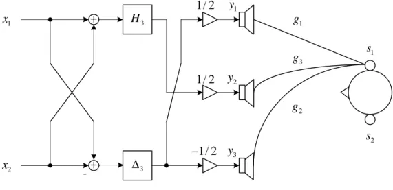
3 3 0 1 0 1 1 1 1 0 0 1 1 2 0 1 H z z ⎡ ⎤ ⎡ ⎤ ⎡ ⎤ ⎢ ⎥ = _{⎢ ⎥⎢ ⎥ ⎢ ⎥} Δ _⎣ − _⎦ ⎣ ⎦ ⎢ − ⎥ ⎣ ⎦ (3.46)

The structure of this type crosstalk canceller is shown in Figure 3. 9 and the impulse

response of these filters are shown in Figure 3.10 and Figure 3.11. Obviously, this

structure is easier to implement than direct forward type and shuffler form. In addition,

it requires only two filters so that economical realization and less computation can be

achievable.

It should be mentioned that only the sum signal x₁+ is fed to the center x₂

loudspeaker, and only the difference signal ±

(

x₁−x₂

)

is fed to the side loudspeakers. One side gets the same signal as the other side loudspeaker, but inverted in sign.

Feeding the side loudspeakers with opposite sign signals is similar to a dipole,

especially when the side loudspeakers are placed close together as described in [17].

1 y 2 y 3 y 1 x 2 x 1/ 2 1/ 2 1/ 2 − 3 Δ 1 g 3 g 2 g 1 s 2 s 3 H

Figure 3.9 The simplified shuffler structure of crosstalk canceller for three loudspeakers arrangement.

0 20 40 60 80 100 120 140 160 180 200 -5 -4 -3 -2 -1 0 1 2 3 4 5x 10 -4 Samples M a gni tud e Time domain H₃(z) 0 20 40 60 80 100 120 140 160 180 200 -6 -4 -2 0 2 4 6x 10 -4 Samples M a gni tud e Time domain Delta 3(z)

Figure 3.10 The impulse response of the filterH . ₃

3.2.5 A Simplified Shuffler Form of Four Loudspeakers

Arrangement

Similarly, we can extend to four loudspeakers and derive the simplified shuffler

form. In this case, we deliver the binaural signals to listener via four loudspeakers as

shown in Figure 3.12. Under symmetric arrangement, the acoustic matrix G is a 2 4×

matrix and the crosstalk canceller matrix C is a 4 2× matrix as shown below

( )

1

( )

_{( )}

2

_{( )}

( )

3

( )

_{( )}

4

_{( )}

( )

4 3 2 1 g z g z g z g z z g z g z g z g z ⎡ ⎤ = ⎢ ⎥ ⎣ ⎦ G (3.53)

( )

( )

( )

( )

( )

( )

( )

( )

( )

1 4 2 3 3 2 4 1 C z C z C z C z z C z C z C z C z ⎡ ⎤ ⎢ ⎥ ⎢ ⎥ =_{⎢ ⎥} ⎢ ⎥ ⎢ ⎥ ⎣ ⎦ C (3.54) 4×2 C 1 g g2 g3 g4

In addition, our desired transfer function matrix D is a 2 2× identity matrix. Thus,

we can obtain two equations as follows

( ) ( )

( ) ( )

( ) ( )

( ) ( )

1 1 2 2 3 3 4 4 1 C z g z +C z g z +C z g z +C z g z = (3.55)

( ) ( )

( ) ( )

( ) ( )

( ) ( )

1 4 2 3 3 2 4 1 0 C z g z +C z g z +C z g z +C z g z = (3.56)

By subtracting and adding Eq. (3.55) and Eq. (3.56), we have

( )

( )

(

)

(

( )

( )

)

(

( )

( )

)

(

( )

( )

)

( )

( )

(

)

(

( )

( )

)

(

( )

( )

)

(

( )

( )

)

1 4 1 4 2 3 2 3 1 4 1 4 2 3 2 3 1 1 g z g z C z C z g z g z C z C z g z g z C z C z g z g z C z C z ⎧ − − + − − = ⎪ ⎨ + + + + + = ⎪⎩ (3.57)

Next, we choose C₂

( )

z =C₃

( )

z and C₂

( )

z +C₃

( )

z =1

(

g₂

( )

z +g₃

( )

z

)

so that

( )

( )

(

)

(

( )

( )

)

( )

( )

(

)

(

( )

( )

)

1 4 1 4 1 4 1 4 1 0 g z g z C z C z g z g z C z C z ⎧ − − = ⎪ ⎨ + + = ⎪⎩ (3.58)

We can further obtain

( )

( )

_{( )}

_{( )}

1 4 1 4 1 1 2 C z C z g z g z = − = − (3.59) and

( )

( )

_{( )}

_{( )}

2 3 2 3 1 1 2 C z C z g z g z = = + (3.60)

then one possible solution of crosstalk canceller can be

( )

( )

( )

( )

( )

( )

( )

( )

( )

( )

( )

( )

( )

( )

( )

( )

( )

1 4 1 4 2 3 2 3 2 3 2 3 1 4 1 4 1 1 1 1 1 1 1 2 1 1 g z g z g z g z g z g z g z g z z g z g z g z g z g z g z g z g z − ⎡ ⎤ ⎢ _{− −} ⎥ ⎢ ⎥ ⎢ ⎥ ⎢ _{+ +} ⎥ ⎢ ⎥ = ⎢ ⎥ ⎢ ⎥ + + ⎢ ⎥ ⎢ ₋ ⎥ ⎢ ⎥ − − ⎢ ⎥ ⎣ ⎦ C (3.61)

( )

(

( )

( )

)

( )

( )

(

)

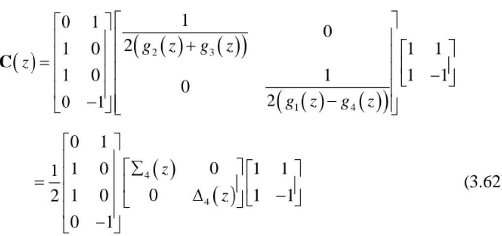
2 3 1 4 1 0 1 0 2 1 0 1 1 1 0 1 1 1 0 2 0 1 g z g z z g z g z ⎡ ⎤ ⎡ ⎤ ⎢ ⎥ ⎢ ⎥ _{+ ⎡ ⎤} ⎢ ⎥ ⎢ ⎥ = _{⎢ ⎥⎢ ⎥} ⎢ ⎥ _⎣ − _⎦ ⎢ ⎥ ⎢ ⎥ ₋ − ⎢ ⎥ ⎣ ⎦ ⎣ ⎦ C

( )

( )

4 4 0 1 0 1 0 1 1 1 0 1 0 1 1 2 0 1 z z ⎡ ⎤ ⎢ _{⎥ ∑⎡ ⎤ ⎡ ⎤} ⎢ ⎥ = _{⎢ ⎥ ⎢ ⎥} ⎢ ⎥_⎣ Δ _⎦⎣ − _⎦ ⎢ ₋ ⎥ ⎣ ⎦ (3.62)

The structure of this type crosstalk canceller is shown in Figure 3.13. Same as the

simplified shuffler form of three loudspeakers setup, it requires only the inversed-sum filter ∑₄

( )

z and the inversed-difference filter Δ₄

( )

z to realize the crosstalk canceller.

It should be mentioned that the approach we propose here is only one possible

solution. There must be lots of different implementation of crosstalk canceller for four

loudspeakers arrangement. 1 y 2 y 3 y 1 x 2 x 4 y 1 g 2 g 3 g 4 g 4 ∑ 4 Δ 1 s 2 s 1 2 1 2 1 2 1 2 −

Figure 3.13 The simplified shuffler structure of crosstalk canceller for four loudspeakers arrangement.

3.2.6 Reduced-Order Modeling

In order to efficiently reduce the orders of the model, we use pole-zero models to

approximate the impulse response of FIR filters. Here, we use Prony appoximation

method to model. Either model can be expressed by the system function:

( )

( )

_{( )}

0

( )

_{( )}

1 1 q k q k q p k p k p B z b k z C z A z a k z − = − = ∑ = = + ∑ (3.63)

The Prony approximation wants to minimize the error:

( )

p

( ) ( )

q

( )

E z =A z x z −B z (3.64)

where x z

( )

is the system’s impulse response that we want to model. Since

( )

0

q

b n = for n> , we may write the error explicitly for each n as follows: q

( )

[ ]

_{[ ]}

1

[ ] [

_{[ ] [}

]

_]

[ ]

1 ; 0,1, , ; p l p q p l p x n a l x n l b n n q e n x n a l x n l n q = = ⎧ + ∑ − − = ⎪ = ⎨ _{+ ∑ − >} ⎪⎩ … (3.65)

Prony approximation begins by finding the coefficients a_p

( )

k that minimize the

square error

[ ]

2

[ ]

[ ] [

]

2 1 1 1 p prony p n q n q l e e n x n a l x n l ∞ ∞ = + = + = =

∑

=

∑

+

∑

− (3.66)

Form this equation, we know the modeled impulse response ˆx n

[ ]

approximates

[ ]

x n without error over the interval

[ ]

0, q . However, there is modeling error

between x n

[ ]

and ˆx n

[ ]

. We will discuss how the modeling error affects the

Chapter 4

Perturbation Analysis

The main disadvantage of crosstalk canceller system is that it is critically dependent

on the listener’s head being in a fixed design position, the so called “sweet-spot”.

Many studies have shown that the lateral movement away from the design position of

as little as a few centimeters results in loss of the 3D audio effect. In this chapter, we

will discuss the robustness of two and three loudspeakers arrangement. The analysis

of shuffler form and simplified shuffler form are our main focus here.

In addition, we will focus on the performances of crosstalk suppression, and see

how perturbations or modeling errors of these inverse filters will affect the crosstalk

suppression in the crosstalk canceller. In the following section, we will discuss which

4.1 Perturbation Analysis for Filter Modeling

First, we will investigate the robustness of crosstalk canceller due to filter modeling

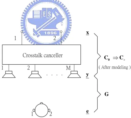
error as shown in Figure 4.1. Ideally, the product of C and ₀ G results in an

identity matrix. After modeling, C becomes ₀ C which means there are modeling ₊

errors inC . Hence, the product of ₊ C and ₊ G is no longer an identity matrix, since the modeling error affects the performance of equalization and crosstalk cancellation.

In this section, we will analyze how the modeling errors affect the performance of two

and three loudspeakers shuffler forms and simplified shuffler form, since their

structures are similar.

0 C e x + ⇒ C y G

Figure 4.1 The geometry of crosstalk cancellation system for multiple loudspeakers after filter modeling

4.1.1 Analysis on Shuffler Form of Two Loudspeakers Setup

From Figure 3.2, we can derive the relation between Y and X in a matrix form.

1 1 2 2 1 2 Y X Y X ∑ +Δ ∑ −Δ ⎡ ⎤ ⎡ ⎤⎡ ⎤ = ⎢ ⎥ ⎢_{∑ −Δ ∑ +Δ}⎥⎢ ⎥ ⎣ ⎦ ⎣ ⎦ ⎣ ⎦ (4.1)

After modeling, the filters ∑ and Δ will be changed to be ∑ and ₊ Δ with ₊

modeling error e and _s,1 e_d,1, respectively, so that the relation between Y₊ and X can be written as follows: ,1 1 ,2 2 1 2 Y X Y X + + + + + + + + + + ∑ +Δ ∑ −Δ ⎡ ⎤ ⎡ ⎤ ⎡ ⎤ = ⎢ ⎥ ⎢_{∑ −Δ ∑ +Δ} ⎥ ⎢ ⎥ ⎣ ⎦ ⎣ ⎦ ⎣ ⎦ ,1 ,1 ,1 ,1 1 ,1 ,1 ,1 ,1 2 1 2 s d s d s d s d e e e e X e e e e X ∑ + + Δ + ∑ + − Δ − ⎡ ⎤ ⎡ ⎤ = ⎢_{∑ + − Δ − ∑ + + Δ +} ⎥ ⎢ ⎥ ⎣ ⎦ ⎣ ⎦ (4.2)

where Y_+,1 and Y_+,2 represent the perturbed signals sent to the loudspeaker pair. The modeling errors after crosstalk cancellation can be expressed as follows:

,1 ,1 ,1 ,1 1 2, ,1 ,1 ,1 ,1 2 1 2 s d s d Shuffler s d s d e e e e g E e e e e g + − ⎡ ⎤ ⎡ ⎤ = ⎢ _{− +} ⎥ ⎢ ⎥ ⎣ ⎦ ⎣ ⎦ (4.3)

Now, we begin the analysis. First, we factorize the filters ∑ and Δ as shown

below 1 2 1 1 1 1 1 g g g F ∑ = = ⋅ + + (4.4) 1 2 1 1 1 1 1 g g g F Δ = = ⋅ − − (4.5) In Eq. (4.4) and Eq. (4.5), we let

2 1 g F g = (4.6)

1 x 2 x 2 y 1 y 1 2 1 2 1 g 2 g 1 s 2 s 1 1 F+ 1 1 F− 1 1 g 1 1 g

Thus, we can obtain the structure as shown in Figure 4.2. It should be mentioned that

we focus on the perturbation of F due to filter modeling so that we assume there are no modeling errors in 1 g . By utilizing Taylor series, we have ₁

( )

1 1 1 1 n n F g ∞ = ⎡ ⎤ ∑ = ⋅ +_⎢ − _⎥ ⎣

∑

⎦ (4.7) 1 1 1 1 n n F g ∞ = ⎡ ⎤ Δ = ⋅ +_{⎢ ⎥} ⎣

∑

⎦ (4.8) After low order filter design, F becomes F₊ with filter modeling error e, i.e.

e=F₊− (4.9) F Therefore, we have 1 1 1 1 g F + + ∑ = ⋅ +

(

) (

) (

2

)

3 1 1 1 F e F e F e g ⎡ ⎤ = ⋅ −_⎣ + + + − + + _⎦

( ) (

)

1 1 1 1 1 n n n F e g ∞ = ⎡ ⎤ = ⋅ +_⎢ − + _⎥ ⎣

∑

⎦ (4.10)

Using binomial series, we can obtain

( )

1 0 1 1 1 1 n n _{k n k} n k n e F k g ∞ − + = = ⎡ ⎛ ⎞ ⎤ ∑ = ⋅ +_⎢ − _{⎜ ⎟ ⎥} ⎝ ⎠ ⎣

∑

∑

⎦

( )

( )

1 1 1 1 1 1 1 n n n _{k n k} n n k n F e F k g ∞ ∞ − = = = ⎡ ⎛ ⎞ ⎤ = ⋅ +_⎢ − + − _{⎜ ⎟ ⎥} ⎝ ⎠ ⎣

∑

∑∑

⎦ (4.11) Similarly, 1 1 1 1 g F + + Δ = ⋅ − 1 1 1 1 1 1 n n k n k n n k n F e F k g ∞ ∞ − = = = ⎡ ⎛ ⎞ ⎤ = ⋅ +_⎢ + _{⎜ ⎟ ⎥} ⎝ ⎠ ⎣

∑

∑∑

⎦ (4.12) We then have ,1 s e = ∑ − ∑ ₊

( )

1 1 1 1 1 n n k n k n k n e F k g ∞ − = = ⎛ ⎞ = ⋅ − _{⎜ ⎟} ⎝ ⎠

∑∑

(

2 2 2 3

)

1 1 2 3 3 e eF e eF e F e g = ⋅ − + + − + − + (4.13) Assume

(

2eF−e

)

(

e2−3eF2+3e F2 − +e3

)

so that

(

)

,1 1 1 2 1 s e F e g ≅ ⋅ − (4.14) and ,1 d e = Δ − Δ ₊ 1 1 1 1 n k n k n k n e F k g ∞ − = = ⎛ ⎞ = ⋅ _{⎜ ⎟} ⎝ ⎠

∑∑

(

2 2 2 3

)

1 1 2 3 3 e eF e eF e F e g = ⋅ + + + + + + (4.15)

(

)

,1 1 1 2 1 d e F e g ≅ ⋅ + (4.16) Thus, the modeling error vector can be written as follows

1 2, 2 1 2 1 2 Shuffler g Fe e E g e Fe g − ⎡ ⎤ ⎡ ⎤ ≅ _{⎢ ⎥⎢ ⎥} − ⎣ ⎦ ⎣ ⎦ (4.17)

To further simplify this analysis, we will assume vectors are reduced to scalars,

1 1

g = and g₂ = to account for interaural intensity difference. Hence, F rr = and

the error vector can be rewritten as

2, 2 1 2 Shuffler re e E e re r − ⎡ ⎤ ⎡ ⎤ ≅ ⎢₋ ⎥ ⎢ ⎥ ⎣ ⎦ ⎣ ⎦

(

2

)

2 1 er e r ⎡ ⎤ = ⎢ ⎥ − ⎢ ⎥ ⎣ ⎦ (4.18) The first element of this error vector indicates the error of equalization part and the

second element represents the error of crosstalk part due to the filter modeling. In [20],

the author has investigated the perturbation analysis on direct forward type 2. The

error vector can be derived as

2 2 0 1 1 0 1 e E e r r ⎡ ⎤ ⎡ ⎤ = _{⎢ ⎥ ⎢ ⎥} − _{⎣ ⎦ ⎣ ⎦} 1 ₂ 1 er e r ⎡ ⎤ = _{⎢ ⎥} − _{⎣ ⎦} (4.19) It is difficult to compare which structure has better immunity of the perturbation. We

4.1.2 Analysis on Shuffler Form of Three Loudspeakers

Arrangement

Also, we take the same analysis on shuffler form of three loudspeakers arrangement

and derive the modeling error vector for comparison. In the same way, we derive the

relation between Y and X in the shuffler form crosstalk canceller of three loudspeakers

arrangement as follows:

(

)

(

)

(

)

(

)

2 2 2 2 1 1 2 2 2 2 3 2 2 2 2 1 1 2 2 1 1 2 2 Y X Y C C X Y ⎡ _{∑ +Δ ∑ −Δ} ⎤ ⎢ ⎥ ⎡ ⎤ ⎢ ⎥ ⎡ ⎤ ⎢ ⎥ = ⎢ ⎥ ⎢ ⎥ ⎢ ⎥ _{⎣ ⎦} ⎢ ⎥ ⎢ ⎥ ⎣ ⎦ _{⎢ ∑ −Δ ∑ +Δ ⎥} ⎣ ⎦ (4.20)

After modeling, the filters ∑ , ₂ C and ₂ Δ will be changed to be ₂ ∑ , _+,2 C_+,2 and

,2 +

Δ with modeling error es,2 , ec,2 anded,2, respectively, so that the relation

between Y₊ and X can be written as follows:

(

) (

)

(

) (

)

,2 ,2 ,2 ,2 ,1 1 ,2 ,2 ,2 2 ,3 ,2 ,2 ,2 ,2 1 1 2 2 1 1 2 2 Y X Y C C X Y + + + + + + + + + + + + + ⎡ _{∑ +Δ ∑ −Δ} ⎤ ⎢ ⎥ ⎡ ⎤ ⎢ ⎥ ⎡ ⎤ ⎢ _{⎥ = ⎢} ⎥ ⎢ ⎥ ⎢ ⎥ _{⎣ ⎦} ⎢ ⎥ ⎢ ⎥ ⎣ ⎦ _{⎢ ∑ −Δ ∑ +Δ ⎥} ⎣ ⎦

(

) (

)

(

) (

)

2 ,2 2 ,2 2 ,2 2 ,2 1 2 ,2 2 ,2 2 2 ,2 2 ,2 2 ,2 2 ,2 1 1 2 2 1 1 2 2 s d s d c c s d s d e e e e X C e C e X e e e e ⎡ _{∑ + + Δ + ∑ + − Δ −} ⎤ ⎢ ⎥ ⎢ ⎥ ⎡ ⎤ =_⎢ + + _{⎥ ⎢ ⎥} ⎣ ⎦ ⎢ ⎥ ∑ + − Δ − ∑ + + Δ + ⎢ ⎥ ⎣ ⎦ (4.21)

whereY_+,1, Y_+,2 and Y_+,3 represent the perturbed signals sent to the loudspeakers. Then the modeling error after crosstalk cancellation can be expressed as follows:

1 y 2 y 3 y 1 x 2 x 1/ 2 1/ 2 1 g 2 g 3 g s1 2 s 1 1 F+ 1 1 F+ 1 1 F− 1 1 g 1 1 g 1 1 g 1 H 2 H

(

)

(

)

(

)

(

)

1 ,2 ,2 ,2 ,2 ,2 3, 3 ,2 ,2 ,2 ,2 ,2 2 1 1 2 2 1 1 2 2 s d c s d shuffler s d c s d g e e e e e E g e e e e e g ⎡ _{+ − ⎤ ⎡ ⎤} ⎢ _{⎥ ⎢ ⎥} = ⎢ _{⎥ ⎢ ⎥} ⎢ _{− +} ⎥_{⎢ ⎥} ⎣ ⎦ ⎢ ⎥ ⎣ ⎦ (4.22)

Now, we begin the analysis. First, we factorize the filters ∑ , ₂ C and ₂ Δ as ₂

follows:

(

1

)

2 2 2 ₂ 2 1 1 2 3 ₃ 1 2 1 1 1 1 2 1 2 g g g F g g g _g g g + ∑ = = ⋅ ⋅ + + + ⎛ ⎞ + ⎜ ₊ ⎟ ⎝ ⎠ (4.23)

(

)

(

)

(

)

1 2 3 3 2 2 ₂ 2 ₂ 1 1 2 3 1 2 3 1 1 1 2 2 g g g g C g F g g g g g g + = = ⋅ ⋅ + + + + + (4.24) 2 1 2 1 1 1 1 1 g g g F Δ = = ⋅ − − (4.25) where F is described in section 4.1.1. Thus, we can obtain the structure as shown in Figure 4.3. The filters H and ₁ H in Figure 4.3 are shown below ₂

(

)

(

)

1 2 3 1 2 1 2 3 2 2 ₂ 1 2 3 1 1 2 2 H g g g g g g H g g g ⎧ ₌ ⎪ _{⎛ ⎞} ⎪ _{+ ⎜ ⎟} ⎪ ₊ ⎝ ⎠ ⎨ ⎪ ₊ ⎪ ₌ ⎪ + + ⎩ (4.26)

By utilizing Taylor series, we have

( )

2 2 1 1 ₃ 1 2 1 1 1 1 2 n n F g _g g g ∞ = ⎡ ⎤ ∑ = ⋅ ⋅ +_⎢ − _⎥ ⎣ ⎦ ⎛ ⎞ + ⎜ ₊ ⎟ ⎝ ⎠

∑

(4.27)

(

)

(

)

( )

1 2 3 2 2 ₂ 1 1 _{1 2 3} 1 1 2 n n g g g C F g _{g g g} ∞ = + ⎡ ⎤ = ⋅ ⋅ +_⎢ − _⎥ + + ⎣

∑

⎦ (4.28) 2 1 1 1 1 n n F g ∞ = ⎡ ⎤ Δ = ⋅ +_{⎢ ⎥} ⎣

∑

⎦ (4.29) After low order filter design, F becomes F₊ with filter modeling error e as described in Eq. (4.9) so that we have

,2 2 1 ₃ 1 2 1 1 1 1 1 2 g _g F g g + + ∑ = ⋅ ⋅ + ⎛ ⎞ + ⎜ ₊ ⎟ ⎝ ⎠

(

) (

) (

2

)

3 2 1 ₃ 1 2 1 1 1 1 2 F e F e F e g _g g g ⎡ ⎤ = ⋅ ⋅ −_⎣ + + + − + + _⎦ ⎛ ⎞ + ⎜ ₊ ⎟ ⎝ ⎠

( ) (

)

2 1 1 ₃ 1 2 1 1 1 1 1 2 n n n F e g _g g g ∞ = ⎡ ⎤ = ⋅ ⋅ +_⎢ − + _⎥ ⎣ ⎦ ⎛ ⎞ + ⎜ ₊ ⎟ ⎝ ⎠

∑

(4.30)

Using binomial series, we can obtain

( )

( )

,2 2 1 1 1 1 ₃ 1 2 1 1 1 1 1 2 n n n k n k n n k n F e F k g _g g g ∞ ∞ − + = = = ⎡ ⎛ ⎞ ⎤ ∑ = ⋅ ⋅ +_⎢ − + − _{⎜ ⎟ ⎥} ⎛ ⎞ ⎣ ⎝ ⎠ ⎦ + ⎜ ₊ ⎟ ⎝ ⎠

∑

∑∑

(4.31)