可動態擴充之數位訊號處理核心於系統單晶片內之整合架構研究(III)

(1)

行政院國家科學委員會專題研究計畫成果報告

可動態擴充之數位訊號處理核心於系統單晶片內之整合架

構研究(3/3)

計畫類別：個別型計畫計畫編號： NSC94-2213-E-009-001- 執行期間： 94 年 08 月 01 日至 95 年 07 月 31 日執行單位：國立交通大學資訊工程學系(所) 計畫主持人：鍾崇斌共同主持人：單智君計畫參與人員：吳奕緯、黃士嘉、田濱華、林聖勳、陳志遠報告類型：完整報告處理方式：本計畫可公開查詢

中華民國 95 年 10 月 31 日

(2)

行政院國家科學委員會專題研究計畫成果報告

可動態擴充之數位訊號處理核心於系統單晶片內之整合架

構研究(3/3)

Reconfigurable Computing for Complex Arithmetic Systems

― Using Rendering as an Example (3/3)

計畫編號： NSC94-2213-E-009-001-

執行期間： 94 年 08 月 01 日至 95 年 07 月 31 日

計畫主持人：鍾崇斌國立交通大學資訊工程系

共同主持人：單智君國立交通大學資訊工程系

計畫參與人員：吳奕緯、黃士嘉、田濱華、林聖勳、陳志遠

中文摘要

伴隨著IC 製程的進步，現今的在一個晶片中塞入數百萬以上電晶體以經是件滿容易的事，其中可能包含CPU、Memory、DSP、Flash 等，形成完整系統，即所謂晶片系統(System-on-Chip，SoC)，亦可稱為系統晶片。然而若將 SoC 應用到嵌入式系統時，電源消耗與執行效能往往是個最直接遭遇到的課題。因此，我們在本計畫中，便針對 SoC 中電源消耗與執行效能這兩議題提出相對應的解決方法。通常對於 SoC 系統的電源消耗而言，處理器往往是佔最大的比重。對此，我們在第一年度中針對目前嵌入式處理器(embedded processor)在指令匯流排 (instruction bus) 上的省電需求，提出一同時兼具暫存器重新標記 (register relabeling)以及指令編碼(instruction encoding) 優點的演算法，使編碼後的資料在 instruction bus 上傳送時的位元觸發(bit toggle) 數更小。實驗數據顯示，我們提出的演算法比起單純只有register relabeling 減少約 50%的位元轉換(bit transition) 數；比起單純只有instruction encoding 的方法減少約 19%的 bit transition 數。

在第二年中，我們又針對 embedded processor 提出兩個減低電源消耗的方

法。分別為 ARM9 微處理機之省電設計與低耗電指令快取記憶體（instruction

cache，I-Cache）。根據分析 ARM 程式在 ARM9TDMI 處理機架構執行流程發現，處理機中的運算單元（乘法器、ALU、shifter）並不會同時使用到，也就是說運算單元不需一直保持於忙碌狀態，這種狀況提供了省電設計的可能。因此，若能將不需使用的運算單元關閉，則可節省不必要的能量消耗。成果顯示平均而言可以節省 30~60%之 ALU 與 shifter 的 switching power，另外可節省 99%之 multiplier 的 switching power。在 I-Cache 的使用上，程式在執行時 cache line 的

使用個數是不多的，因此我們也可把這些沒有使用到的cache line 轉成低電壓模

式，以降低I-Cache 的靜態功率消耗。然而調低 cache line 電壓所付出的代價是，

當系統需要存取該cache line 時，則需要較多時間延遲。因此，若我們能準確的

預測每一條cache line 需要被存取的時機，我們就能在耗電與存取時間上取得一

(3)

靜態功率消耗。

在第三年的部分，我們則針對embedded processor 提出一個增進其執行效能

的方法，稱之為延伸指令集(instruction set extension, ISE)。ISE 的基本概念就是根據目前程式的特性，找出常被執行的一些指令樣式(instruction pattern)，並在 processor 增加額外的硬體來執行這些 instruction patterns，藉此加速程式的執行。而這裡所說的instruction patterns 便可由新增的 instructions 來取代，也就是 ISEs。

因此，ISE 可被視為是一種有效的方式可以滿足在許多應用上不斷增加的電路以

及速度的需求。ISE 產生的流程通常包含了 ISE exploration 以及 ISE selection 兩

個步驟，在ISE exploration 的步驟中，為了要達到最高的加速效果，大多數的研

究都直接使用速度最快的實做方式來實做每一個在特殊的功能單元(application specified function unit, ASFU)中的基本運算，而 ASFU 也就是複雜執行延伸指令集的功能單元，儘管如此，最快速的實作方式卻不一定是最好的選擇，在選擇 ASFU 中的運算的實作方式時，有兩點重要的考量：(1)ASFU 的執行時間必須符合管線時間的限制，也就是必須與原本管線時脈的整數倍相同，並且在(1)的前提下，(2)ASFU 必須使用最少的額外面積，為了要滿足這些考量，我們提出了一

個ISE Exploration 的演算法不只可以探索 ISE 候選者，也同時考慮了它們的實作

方式以期能夠減少最多的執行時間，並且在此同時使用較少的面積。使用 Mibench 的模擬結果顯示，與沒有考量管線時間的 ASFU 比較，這個方法可以額外節省 35.28%、15.92%以及 22.41%(最大、最小以及平均)的面積，而且最多只有 1.06%的效能損失，模擬的結果更進一步的顯示我們的方法在足夠小的例子中，找出來的結果與最佳解相當接近，但卻節省了相當多的計算時間。關鍵詞：系統單晶片、低耗電快取記憶體、嵌入式處理器、暫存器重新標記、指令編碼、延伸指令集

Abstract

The low power dissipation and high performance achievement are the most crucial challenges in designing system-on-chip (SOC), especially for an embedded system. Since all of these embedded systems are battery-operated, reducing the SOC power dissipation to extend the battery life therefore is important. On the other hand, achieving high performance is another critical issue in designing SoC. Because most power is consumed by embedded processor in most SOC systems, we propose several methods to reduce power consumption and increase execution performance for the embedded processor in this report.

In first year, we present an algorithm, which comprises advantages of register relabeling and instruction encoding, to reduce power consumption of instruction bus. The simulation results showed that our algorithm can reduce over 50% and 19 % of bit transitions than register relabeling and instruction encoding, respectively.

In second year, we propose 2 schemes, are ARM9 low power mechanism and low power instruction cache (I-Cache) respectively, to reduce power consumption in

(4)

the embedded processor. Most operation units, such as ALU, multiplier and Shifter, would not be used at same time according to application profiles from ARM9. Such phenomenon provides a feasible way to reduce processor power dissipation. In this report, we propose a method to turn on/off unused parts of operation units to reduce processor power dissipation. Our simulation shows that our proposed method reduces 30~60% and 99% switching power in ALU/shifter and multiplier respectively. In our observation, only one cache line is accessed in the I-Cache at any cycle. Other unused cache line can hence be turned to low power mode to reduce I-Cache’s static power dissipation. But the cache accessing time would increase, if the processor accesses a cache line in low power mode. Thanks to branch target buffer (BTB), the processor easily predicts the next one and two instruction address and turns these cache lines corresponding to this instruction addresses to active mode in advance. By the same way, the processor predicts whether a cache line will be used in the future. If no, this cache line would be turned to the low power mode. Our simulation shows that our proposed method reduces 80% static power in I-Cache.

Instruction set extension (ISE) is an effective way to meet the growing efficiency demands for both circuit and speed in many applications. In third year, we propose an ISE generation algorithm to improve the execution performance of embedded processor. Because most applications frequently execute the several instruction patterns, grouping these instruction patterns into new instructions, i.e. instructions in ISE, is an effective way to enhance the performance. For simplicity, instruction(s) in ISE is called ISE(s) hereinafter. ISEs are realized by application specific functional units (ASFU) within the execution stage of the pipeline.

ISE generation flow usually consists of ISE exploration and ISE selection phases. In ISE exploration, in order to achieve the highest speed-up ratio, most works deploy the fastest implementation option for each operation in application specific functional unit (ASFU) which executes instruction in ISEs. Nevertheless, the fastest implementation option may be not the best choice. Two considerations are important in selecting an implementation option for each operation in ASFU: (1) the execution time of an ASFU should meet pipestage timing constraint, i.e. fit to an integral number of original pipeline cycles; and (2) under (1), the ASFU should use the least silicon area. To conform to these considerations, we propose an ISE exploration algorithm which not only explores ISE candidates but also their implementation options to minimize the execution time meanwhile use less silicon area. Results with MiBench indicate that the approach achieves up to 35.28%, 15.92% and 22.41% (max., min. and avg.) of further reduction in extra silicon area usage and only has maximally 1.06% performance loss compared with the approach without the consideration of pipestage timing constraint for ASFU. Furthermore, simulation

(5)

results also show that our approach is very close to optimal one, but takes much less computing time.

Keyword: SoC, low power memory, embedded processor, register relabeling, instruction encoding and instruction set extension

(6)

目

錄

摘要...1 1. 簡介...2 2. 相關研究與背景說明...5 3. ISE Exploration...9 4. 實驗結果...17 5. 結論...25 6. 計畫成果自評...26 7. 參考資料...26

(7)

行政院國家科學委員會專題研究計畫成果報告

可動態擴充之數位訊號處理核心於系統單晶片內之整合架

構研究(3/3)

Reconfigurable Computing for Complex Arithmetic Systems

― Using Rendering as an Example (3/3)

計畫編號： NSC94-2213-E-009-001-

執行期間： 94 年 08 月 01 日至 95 年 07 月 31 日

計畫主持人：鍾崇斌國立交通大學資訊工程系

共同主持人：單智君國立交通大學資訊工程系

計畫參與人員：吳奕緯、黃士嘉、田濱華、林聖勳、陳志遠

摘要

A new algorithm for instruction set extension (ISE) exploration with considering pipestage timing constraint is proposed in this paper. In order to achieve the highest speed-up ratio, most works deploy the fastest hardware implementation option to execute instruction(s) in ISE. For simplicity, instruction(s) in ISE is called ISE(s). Nevertheless, the fastest hardware implementation option may not be the best choice. Two considerations are important in selecting a hardware implementation option for each operation within ISE: (1) the execution time of an ISE should meet pipestage timing constraint, i.e. fit to an integral number of original pipeline cycles; and (2) under (1), the ISE should use the least silicon area. To conform to these considerations, the proposed ISE exploration algorithm explores not only ISE candidates but also their hardware implementation option. Compared to previous work, the proposed algorithm minimizes the silicon area cost and further reduces the execution time. Results with MiBench indicate that under same number of ISE, our approach achieves 69.43%, 1.26% and 33.8% (max., min. and avg.) of further reduction in silicon area and also has maximally 1.6% performance improvement compared with the previous work. Furthermore, simulation results also show that our approach is very close to optimal one in small cases, but takes much less computing time.

(8)

1. 簡介

Instruction set extension (ISE) is an effective means of meeting the growing efficiency demands for both circuit and speed in many applications. Currently, the growing number of commercial products is marked, such as Tensilica Xtensa [1], ARC ARCtangent [2], MIPS CorExtend [3] and Nios II [4]. Because most applications frequently execute the several instruction patterns, grouping these instruction patterns into new instructions, i.e. instructions in ISE, is an effective way to enhance the performance. For simplicity, instruction(s) in ISE is called ISE(s) hereinafter. ISEs are realized by application specific functional units (ASFU) within the execution stage of the pipeline. Notably, since this work adopts a load-store architecture, the ASFU cannot access data directly from main memory.

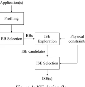
The ISE design flow, as illustrated in Figure 1, comprises application profiling, basic block (BB) selection and ISE generation which consists of ISE exploration as well as selection phases. After profiling, basic blocks are selected as the input of ISE exploration based on their execution time. ISE exploration explores legal instruction patterns as ISE candidates, which have to conform to predefined physical constraints, including ISA format, pipestage timing and instruction/operation types. In other words, ISE exploration determines which operation in basic block should be implemented in hardware (i.e. ASFU) or in software (i.e. executed in CPU core). In addition to exploring ISE candidate(s), the proposed algorithm also explores the hardware implementation options of all operations in ISE candidates. After generating ISE candidates, ISE selection chooses as many ISEs as possible among ISE candidates under predefined physical constraints, which are silicon area and ISA format. In this paper, we only focus on ISE exploration; therefore, the algorithms of ISE selection would not be addressed. Interesting readers could refer ISE selection to [9, 15 and 16] for details.

(9)

Profiling

BB Selection _ExplorationISE

ISE Selection Application(s) ISE(s) Physical constraints BBs ISE candidates

Figure 1: ISE design flow

Several important physical constraints, e.g., pipestage timing, instruction set architecture (ISA) format, register file, convex and silicon area, should be considered during exploring ISE candidates. These physical constraints are described as follows: Pipestage Timing

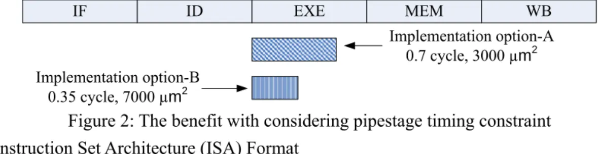
The pipestage timing constraint refers to a situation in which the execution time of ASFU should fit in the original pipestage, i.e. the execution time of ASFU should be an integral number of original pipeline cycles. Many operations in ASFU often have multiple hardware implementation options owing to different area and speed requirements. In ISE exploration, to achieve the highest speed-up ratio, most works [XXXX] usually deploy the fastest hardware implementation option for each operation in ASFU. Nevertheless, the fastest hardware implementation option may not be the best choice unless it can make the execution time of ASFU to fit in or to be as close as possible to the original pipestage. Restated, an ASFU using miser hardware implementation option is better choice due to the manufacturing cost benefit, if it has same execution time reduction with the one using the fastest hardware implementation option. From another perspective, under the same silicon area constraints, designers can employ more ISEs to achieve higher performance improvement than previous works, if the miser implementation option is adopted. Figure 2 is an example to explain the benefit of considering pipestage timing constraint. Assume that there are two hardware implementation options for an ISE, namely implementation option-A (IO-A) and implementation option-B (IO-B). The silicon area and execution time of IO-A are 3000 µm2 and 0.7 cycle, respectively; as well as IO-B, 7000 µm2 and 0.35 cycle. Obviously, IO-B has faster execution time than IO-A. Nevertheless, under pipestage timing constraint, both of them have same performance improvement, but IO-A consumes less silicon area. This is why considering pipestage timing constraint can bring benefit in silicon area saving;

(10)

meanwhile, maintain the same level of performance. IF ID EXE MEM WB Implementation option-A 0.7 cycle, 3000 µm2 Implementation option-B 0.35 cycle, 7000 µm2

Figure 2: The benefit with considering pipestage timing constraint Instruction Set Architecture (ISA) Format

The ISA format represents two constraints. The first constraint limits the number of input/output operands employed by an ISE. The second constraint is the number of ISEs and is usually used in ISE selection. That is, the number of ISEs generally cannot exceed the number of unused opcodes. However, perhaps some people would question why not use multiple instructions to overcome both constraints. The reason is that using multiple instructions to represent one ISE may increase ISE fetching latency. This leads to lengthening the execution time of ISE. The trade-off between execution time reduction and the number of opcodes as well as operands is another problem. We do not intend to address this problem in this paper.

Register File

The Register file constraint resembles the first constraint of the ISA format. Under the register file constraint, the number of input/output operands adopted by an ISE cannot exceed the number of read/write ports of the register file.

Convex

The convex constraint is that the ISE’s output cannot connect to its input via other operations not grouped in ISE. In other words, if no path exists from a operation u ISE A to another operation v ISE A involving a operation w∉ ISE A, then ISE A is convex. Figure 3 illustrates an example of the convex and non-convex ISEs. The convex constraint is needed to ensure that a feasible scheduling exists. On the other hand, an ISE violating the convex constraint would have less or no execution time reduction. 3 4 1 2 Non-convex 3 4 1 2 Non-convex 3 4 1 2 Convex 3 4 1 2 Convex

Figure 3: The convex and non-convex ISEs Silicon Area

(11)

The silicon area constraint limits the silicon area usage for a single ISE to a predefined or reasonable size. In ISE selection, the silicon area constraint also restricts the total silicon area utilized by all ASFUs.

In ISE exploration, many investigations may overlook pipestage timing constraint such that causes unnecessary waste of silicon area. To handle pipestage timing and other constraints above, we propose a new ISE exploration algorithm. The proposed algorithm is derived from the ant colony optimization (ACO) algorithm [5, 6 and 7]. In contrast with previous studies [8], the proposed algorithm explores not only ISE candidates, but also their hardware implementation option, thus reducing the silicon area and minimizing the execution time. Results with MiBench reveal that under same number of ISE, the proposed approach achieves 69.43%, 1.26% and 33.8% (max., min. and avg.) of further reduction in silicon area, and also has maximally 1.6% performance improvement over the previous work [8]. Conversely, under the same silicon area constraint, the proposed approach reaches up to 3.85%, 0.97% and 2.17% (max., min. and avg.) more speedup than the previous one [8]. Moreover, simulation results also demonstrate that the proposed approach is extremely close to the optimal scheme, but takes much less computing time.

This study has the following contributions:

1. An ISE exploration algorithm is proposed, which explores not only ISE candidates, but also their hardware implementation options, and thus reducing the silicon area cost.

2. The proposed ISE exploration algorithm not only significantly lowers silicon area cost, but also enhances performance over the previous algorithm.

3. The proposed ISE exploration algorithm can explore a search space comprising hundreds of instructions in a few minutes, and has a near-optimal solution. The rest of this work is structured as follows. Section 2 studies the previous related work and background of Ant Colony Optimization Algorithm. Section 3 then presents the proposed approach. Next, Section 4 presents the simulation results and discussion. Conclusions are finally drawn in Section 5.

2. 相關研究與背景說明

2.1 Relative Works

Pozzi [8] proposed an algorithm, called the exact algorithm, to examine all possible ISE candidates such that it can obtain an optimal solution. The exact algorithm maps the ISE search space, such as a basic block, to a binary tree, and then discards some portion of the tree that violates predefined constraints. Nevertheless,

(12)

this algorithm is highly computing-intensive, so it does not process a larger search space. For instance, if a BB has N operations, and each operation has only one hardware implementation option, then it has 2N possible ISE patterns (legal or illegal). Notably, one ISE candidate may consists of one or multiple legal ISE pattern(s). When N = 100 (the standard case), then the number of possible ISE patterns is 2100. Obviously, this number of patterns cannot be computed in a reasonable time. To decrease the computing complexity, heuristic algorithms derived from genetic [8], Kernighan-Lin (KL) [9] and greedy-like algorithms [10] have been developed.

Yu [11] investigated the effect of various constraints, such as ISA format, hardware area and control flow, for ISE generation. Such constraints restrict the performance improvement of the ISEs. The ISA format limits the number of read and write ports to the register file. The limitation of the control flow is whether the search space of ISE exploration can cross basic block boundaries. To meet time constraint in real-time applications, the operations locating on the worst-case execution path would have higher opportunity to be grouped into ISE than others, as in [12]. This is because the most frequently executed instruction pattern may not contribute execution time reduction to the worst-case execution path. The granularity of each vertex within the search space can be varied from one instruction to multiple subroutine calls [13]. Borin [13] also claims that one search space can consist of multiple basic blocks in their proposed algorithm. From a different perspective, Peymandoust [14] characterized each basic block as a polynomial representation. First, the multiple-input single-output (MISO) algorithm extracts symbolic algebraic patterns from the search spaces, and represents them as polynomials on behalf of ISE candidates. These ISE candidates are then mapped to the polynomial representations of program segments using symbolic algebraic manipulations. Nevertheless, some algorithms [8, 9, 10, 11, 12, 13 and 14] do not consider the pipestage timing constraint, and therefore waste silicon area unnecessarily.

2.2 Background - Ant Colony Optimization (ACO) Algorithm

Basic Idea of Ant Colony Optimization Algorithm

Ant Colony Optimization algorithm is inspired by the behavior of ants in finding paths from the colony to food. This algorithm [1, 2] has been extensively applied to solve many optimization problems.

In the real world, ants wander randomly when they begin to find paths from the colony to food. The ants lay down pheromone on the paths which they have passed through. The density of the pheromone on one path determines the probability that the next ant will pass through this path. Because the pheromone evaporates with time, the shortest path is marched over fastest, and thus has the highest pheromone density.

(13)

After a period of time, an increasing number of ants select the shortest path, causing the density of pheromone on this path gradually grow. Finally, the shortest path is obtained. The shortest path can be treated as the optimal solution for an optimization problem.

Figure 2 depicts an example of ACO. Suppose that 50 ants are going to find food, and can choose from among two paths, namely left-path (left hand side path) and right-path (right hand side path). Left-path is twice as long than right-path, as illustrated in Fig. 2 (a). In Fig. 2, D and P are the number of unit of distance and pheromone, respectively, and t represents the time unit. At t = 0, neither path has pheromone, and the ants choose paths with equal probability. Suppose that 25 ants choose left-path, and 25 ants choose right-path at the beginning of t = 1, as shown in Fig. 2 (b). Every ant leaves one unit of pheromone on the path. At the end of t = 1, 25 ants arrive food source, and another 25 ants are in the middle of left-path. Black spots in Fig. 2 (c) depict the locations of ants at the end of t = 1. Assume that the pheromone evaporates at a rate of 5 units per time unit. The paths ant passed have 20 (=25−5) units of pheromone after evaporation, as displayed in Fig. 2 (c). Then, the ants start walking again at the beginning of t = 2, as demonstrated in Fig. 2 (d). 25 ants return to their colony and another 25 ants arrive food source, at the end of t = 2. The locations (black spots) of ants at the end of t = 2 is shown in Fig. 2 (e). Fig. 2 (f) depicts the number of pheromone units on each path segment after t = 2. At next iteration, right-path has a higher probability of being chosen by ants than left-path owing to the higher pheromone density. After a period of time, an increasing number of ants select right-path due to higher density of pheromone, causing the density of pheromone on right-path grows. Finally, the shortest path, i.e. right-path, is obtained.

(14)

Figure 2: An example of ant colony Why Use the Ant Colony Optimization Algorithm?

ISE exploration is an optimization problem. Many computation models, such as genetic algorithms and simulated annealing, have been successfully adopted to solve many optimization problems. One of those computation models, named ACO, is very similar to the ISE exploration problem that explores not only ISE candidates, but also their hardware implementation options. A computation model that is more similar to the original problem than others should be chosen for minimizing the modification required. In other word, a computation model that more closely resembles the original problem requires less modification than other models do.

The ISE exploration problem is clearly analogous to ACO. Selecting the shortest path among multiple paths in ACO can be viewed as similar to choosing the best implementation option (hardware or software) among different implementation options for each operation in the basic block. One can imagine that different implementation options for all operations in a basic block can be modeled as a tree. An operation can be seen as a node in the tree, and different implementation options are different links between two nodes in the tree. Figure 3, in which O1 is operation 1 as well as SW-IO and HW-IO denote the software and hardware implementation option, respectively, illustrates this concept. In Fig. 3, the ants start from their colony (operation 1) to food (operation m), and make a decision at every node (choose one

P=25→20

Food

Food Food

Ant Colony Ant Colony

25 ants 25 ants

Ant Colony (50 ants)

D=20 D=20 D=10 D=10 25 ants P=25→20 P=25→20 Food Ant Colony 25 ants 25 ants Food Ant Colony 25 ants P=45→40 P=20→15 P=45→40 25 ants Food Ant Colony P=20 P=15 P=40 P=40 Before Start (t=0) (a) Go (t=1) (b) Evaporation (t=1) (c) Go (t=2) (d) Evaporation (t=2) (e) After (t=2) (f) D = Distance, P = Pheromone

(15)

implementation option of each operation). After a period of time, i.e. several iterations, the ants find the shortest path (the dotted line with arrow in Fig. 3) between their colony and food. The shortest path is the optimal solution in ISE exploration.

O 1 H W -IO 1 H W -IO n SW-IO O 2 H W -IO 1 H W -IO n SW -IO O m H W -IO 1 H W -IO n SW -IO O m H W -IO 1 H W -IO n SW -IO Operation 1 Operation 2 Operation m Ant Colony Food

Figure 3: Analogy between ACO and ISE exploration

3. ISE Exploration

ISE exploration in this work not only identifies frequently executed instruction patterns as ISE candidates, but also evaluates hardware implementation options of each operation in ISE candidates to minimize the execution time while using less silicon area. The input and output of ISE exploration algorithm are basic blocks and ISE candidates as well as their hardware implementation options, respectively. The

(16)

implementation option(s) of an operation denote(s) its implementation method(s), and can be roughly divided into two categories, namely hardware and software.

The flow of ISE exploration is briefly described as follows. According to the results of BB selection, each selected basic block is transformed to a data flow graph (DFG). DFG is represented by a directed acyclic graph G(V,E) where V denotes a set of vertices, and E represents a set of directed edges. Every vertex v V is an assembly instruction in the basic block, called an “operation” or “node” hereafter. Each edge (u,v) E from operation u to operation v signifies that the execution of operation v needs the data generated by operation u. Then, an implementation option (IO) table representing all implementation options for an operation is appended to each operation in a DFG. Using the DFG with IO table, ISE exploration algorithm is repeatedly executed until no ISE candidate can be discovered. Significantly, the ISE exploration algorithm identifies at least one ISE candidate at each round. A round usually consists of multiple iterations.

At each iteration, the ISE exploration algorithm initially selects one implementation option in each operation according to a probability value (p), which is a function of trail and merit values. Note that every implementation option has one probability value (p). The meaning of trail is the same with the pheromone in the ACO algorithm, i.e. how many times an implementation option is chosen in previous iterations. The merit value is the benefit of one implementation option being chosen. The trail value of the selected implementation option is increased, while others (i.e. non-selected implementation options) are decreased after making a choice. Restated, the result having the highest merit value can be regarded as a local optimal solution. The trail value guides the current solution to achieve global optimal, and the probability value (p) assists the current solution in departing local optimal. After updating trail values, the algorithm evaluates all implementation options of each operation in DFG, i.e. it computes their merit value using merit function. This process is iteratively performed until convergence criteria are met, i.e. until the probability values (p) of all operations have exceeded a predefined threshold value.

3.1 Implementation option

An operation normally has multiple implementation options, which can be divided into two categories, namely hardware and software. The hardware implementation option means that the operation is included in an ISE and is implemented in additional hardware, i.e. ASFU. Because of different speed and area requirements, most operations usually have multiple hardware implementation options. By contrast, the software implementation option signifies that the operation is performed in the CPU core.

(17)

implementation option (IO) table, is appended to every operation. Each entry in the IO table comprises three fields, namely implementation option, delay and area. The name of implementation option is shown in implementation option field. The execution time and the extra silicon area cost of one implementation option are shown in delay field and area field, respectively. Obviously, using software implementation option requires at least one execution cycle, but does not introduce any extra silicon cost. Conversely, using the hardware implementation option can reduce the number of execution cycle, but increases the silicon area consumed. A new graph G+ is generated after the IO table is appended to G. Figure 3 shows an example of G+, consisting of two operations, A and B.

Figure 3: An example of G+

3.2 Formulation of ISE exploration

ISE exploration explores ISE candidates in G+, and evaluates the implementation options of each operation in ISE candidates. An ISE candidate in G+ is a subgraph S G+. The proposed ISE exploration can be formulated as follows.

ISE exploration: Considering a graph G+, obtain subgraph S G+, and evaluate

the implementation options of vertex v S to minimize the execution cycle count while reducing the silicon area as many as possible under the following constraints:

1. IN(S) ≤ Nin, 2. OUT(S) ≤ Nout, 3. S is convex,

4. Load and store operations∉ S.

IN(S) (OUT(S)) is the number of input (output) values used (generated) by a subgraph S (i.e. an ISE). The user-defined values Nin and Nout denote the read and write ports limitations of the register file, respectively. To conform to the limitation of load-store architecture, the load and store operations are forbidden from being grouped into ISE.

(18)

The main task of the proposed ISE exploration algorithm can be considered as assigning an implementation option (including hardware and software) for each operation in the basic block to minimize the execution time and silicon area cost. Therefore, how to choose a “right” implementation option for an operation is crucial for the proposed ISE exploration algorithm. As with the ACO algorithm, the implementation option is chosen according to its probability value (p). The probability value (p) of an implementation option is the implementation option’s probability of being selected at each iteration of the ISE exploration algorithm. The reason using the probability value (p) is that selecting the implementation option based on its probability value (p) can prevent local optimal solutions. The probability value (px,j) of implementation option j in operation x is a function of the trail and the

merit values, as revealed in Equation (1). The significance of the trail value is identical to that of the pheromone in the ACO algorithm, and reveals the number of times that an implementation option is selected in previous iterations. Here, the trail value of implementation option j of operation x is denoted by trailx,j, and trailx,0 is

designated as the trail value of software implementation option. The trail value, like the pheromone, must be updated at each iteration. The merit value is defined as the benefit of one implementation option being selected, and it is obtained by using the merit function, which is described in detail later. The merit value of implementation option j of operation x is represented by meritx,j, and meritx,0 is designated as the merit

value of the software implementation option. The probability value of implementation option j of operation x (px,j) is derived with:

1 0 and 0 1 1 0 , , , , , ≤ ≤ ≤ ≤ ⋅ − + ⋅ ⋅ − + ⋅ =

∑

= α k j , ) merit α) ( trail (α merit α) ( trail α p _k j j x j x j x j x j x (1)

where k is the number of hardware implementation options in operation x, and α is utilized to determine the relative influence of trail and merit, and

1 0 , =

∑

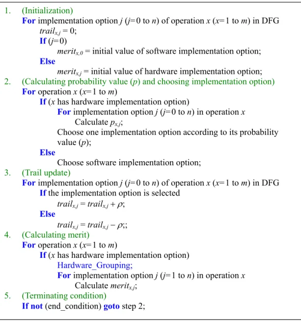
= k j j x p (2) Figure 4 shows the pseudo code of the proposed ISE exploration algorithm. Here, a DFG is assumed to have m (m > 0) operations, each with n (n > 0) implementation options. Initially, i.e. in step 1, the algorithm sets initial values for the trail and merit values of each implementation option of all operations. Notably, the hardware implementation options have higher initial merit values than software ones such that the algorithm could preferentially choose the hardware implementation option at the start of execution to achieve higher performance improvement. In step 2, the algorithm verifies all operations to determine whether they have hardware implementation options. If yes, then the algorithm selects one implementation option

(19)

(including hardware and software) in each operation based on the probability value; if no, then it selects the software implementation option. In Step 3, the algorithm updates the trail value of each implementation option in all operations. The trail value of the chosen implementation option (i.e. the implementation option has been selected in Step 2) is raised with increasing ρ, a positive constant value, while those of others are reduced. Here, ρ is called evaporating factor and very similar to the evaporation rate in ACO. The algorithm in Step 4 derives the merit value of each implementation option in all operations. As in Step 2, the algorithm first checks each operation to determine whether it has a hardware implementation option. If yes, then the algorithm executes the Hardware Grouping function, which determines whether an operation can be grouped with its reachable operations as a virtual ISE candidate. If it can be grouped, then the Hardware-Grouping function adopts this virtual ISE candidate to obtain the execution time and silicon area for every hardware implementation option in this operation. The Hardware-Grouping function is described in detail later. The ISE exploration algorithm then computes the merit value with the merit function. Finally, the ISE exploration algorithm checks the end condition in Step 5. If the end condition is not fulfilled, then the ISE exploration algorithm returns to Step 2 and enters the next iteration; otherwise, it terminates.

The end condition is that for all operations in DFG, the probability value (p) of one of implementation options exceeds P_END, which is a predefined threshold value and is very close to 100%. A larger P_END has a higher opportunity of obtaining a better result, but typically takes a longer time to converge. An implementation option with the probability value (p) larger than P_END is called a taken implementation option. An ISE candidate is a set of reachable nodes (i.e. operations) all of which have taken hardware implementation option.

(20)

Figure 4: ISE Exploration Algorithm Hardware-Grouping

Hardware-Grouping checks whether the operation x can be grouped with its reachable nodes (i.e. operations) as a virtual ISE candidate, and recursively groups operation x with its reachable nodes, which have chosen hardware implementation option in previous iteration, as a virtual ISE candidate, i.e. a virtual subgraph vSx. The

result of Hardware-Grouping of operation x using implementation option j is denoted as vSx,j. Significantly, vSx is the set of all vSx,j (i.e. vSx={ vSx,j | j = 1 to n}), and vSx,0 is

meaningless due to implementation option 0 is the software option. Using vSx,j,

Hardware-Grouping measures the execution time, silicon area and register read/write port usage of vSx,j.The execution time of vSx,j is the critical path time in vSx,j, the

silicon area of vSx,j is the sum of silicon areas used by all operation in vSx,j, and

register read/write port usage is the number of register file read/write ports utilized by 1. (Initialization)

For implementation option j (j=0 to n) of operation x (x=1 to m) in DFG trailx,j = 0;

If (j=0)

meritx,0 = initial value of software implementation option;

Else

meritx,j = initial value of hardware implementation option;

2. (Calculating probability value (p) and choosing implementation option)

For operation x (x=1 to m)

If (x has hardware implementation option)

For implementation option j (j=0 to n) in operation x Calculate px,j;

Choose one implementation option according to its probability value (p);

Else

Choose software implementation option; 3. (Trail update)

For implementation option j (j=0 to n) of operation x (x=1 to m) in DFG

If the implementation option is selected trailx,j = trailx,j + ρ;

Else

trailx,j = trailx,j − ρ;;

4. (Calculating merit)

For operation x (x=1 to m)

If (x has hardware implementation option)

Hardware_Grouping;

For implementation option j (j=1 to n) in operation x Calculate meritx,j;

5. (Terminating condition)

(21)

vSx,j. Notably, cumulating the silicon area used by each operation in vSx,j may not

reflect the silicon area utilized by vSx,j in real; however, it can simplify the calculation

of silicon area, and the cumulating result is the upper bound of silicon area; that is, more silicon area saving can be achieved in real case.

Figure 5: Examples of Hardware-Grouping

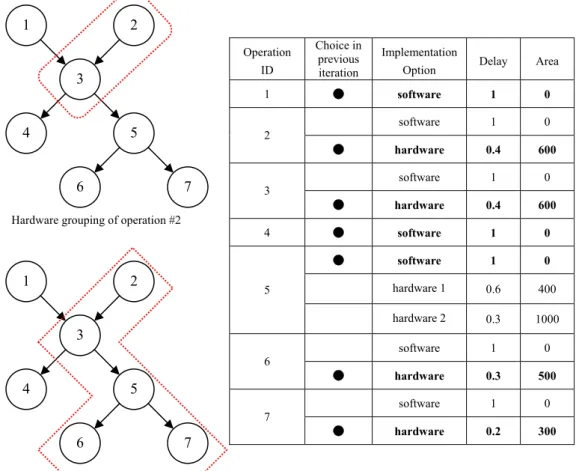
Figure 5 depicts the working of the Hardware-Grouping function. The table in Fig. 5 lists the delay and area of each implementation option of all operations, and specifies the chosen implementation option in the previous selection. In both the top and bottom left of Fig. 5, nodes grouped by a dotted line are treated as a virtual ISE candidate. For operation #2, Hardware-Grouping groups operation #2 and #3 as a virtual ISE candidate, i.e. vS2, as shown in the top left of Fig. 5. Because operation #2

only has one hardware implementation option, vS2 has one evaluation result, namely

vS2,1 (execution time = 0.8, silicon area = 1200). The bottom left of Fig. 5 is another

example, in which Hardware-Grouping groups operation #5 and other nodes, are #2, #3, #6 and #7, as a virtual ISE candidate, i.e. vS5. Since operation #5 has two

hardware implementation options, vS5 has two evaluation results, namely vS5,1

(execution time = 1.7, silicon area = 2400) and vS5,2 (execution time = 1.4, silicon

area = 3000).

Hardware grouping of operation #5 Hardware grouping of operation #2

Operation ID Choice in previous iteration Implementation

Option Delay Area

1 ● software 1 0 software 1 0 2 ● hardware 0.4 600 software 1 0 3 ● hardware 0.4 600 4 ● software 1 0 ● software 1 0 hardware 1 0.6 400 5 hardware 2 0.3 1000 software 1 0 6 ● hardware 0.3 500 software 1 0 7 ● hardware 0.2 300 2 3 4 5 1 7 6 2 3 4 5 1 7 6

(22)

Merit Function

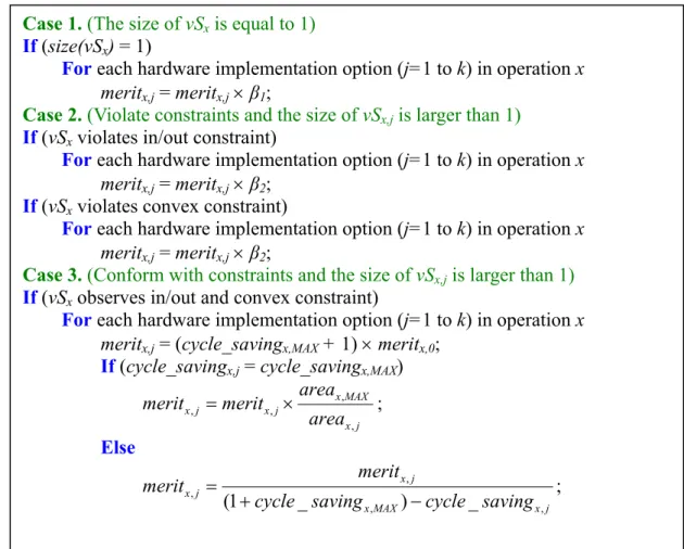
The merit function determines the benefit, i.e. merit value, of different implementation options in an operation. Briefly, the merit function consists of three cases, size checking (case 1), constraints violation determination (case 2) and performance as well as area benefits calculating (case 3). Figure 6 shows the merit function algorithm. Initially, in case 1, the algorithm checks whether size(vSx,j), which

is the number of operation in vSx,j, is equal to 1. Notably, this work assumes that every

operation is one-cycle delay in original processor specification. If a multiple-cycle delay is assumed, then case 1 should be tailored to fit this situation. If size(vSx,j) = 1,

then vSx,j only has one operation x such that the performance cannot be improved.

Therefore, the algorithm multiplies the merit value of every hardware implementation option by a constant β1 (0 < β1 < 1) to lower the chance of it being chosen. The

calculation of the merit function is then terminated. If no, then goto case 2.

Case 2 verifies whether vSx violates input/output port and/or convex constraints.

If yes, then the merit value of each hardware implementation option is multiplied by constant β2 and/or β3 (0 < β2 < 1 and 0 < β3 < 1), reducing the opportunity for

selecting the hardware implementation option, as in case 1. The calculation of the merit function is then terminated. Since operation x may have chance to be grouped in an ISE candidate at the following iterations, the algorithm only divides the merit value of each hardware implementation option by a constant. If the algorithm does not allow the possibility of operation x becoming an operation in an ISE candidate, the optimal solution may also be excluded. If no, then enter case 3.

In case 3, the merit value of implementation option j (meritx,j, j > 0) in operation

x is computed according to (1) the speedup that can be achieved by vSx,j, and (2) the

silicon area utilized by vSx,j. The execution cycle reduction and silicon area of the

virtual subgraph vSx,j is represented by cycle_savingx,j and areax,j, respectively. The

basic concept of case 3 is: (1) if vSx,j can improve the performance, then all hardware

implementation options should have larger merit value than the software one; (2) the merit value should be direct proportion to the execution time reduction, and (3) under the same performance improvement, the hardware implementation option using less silicon area should have larger merit value Accordingly, the merit of software implementation option is always set as a constant, meritx,0, to be a baseline. In case 3,

the algorithm first sets the merit value of implementation option j as the product of cycle_savingx,MAX + 1 and meritx,0 ,where cycle_savingx,MAX is the maximal execution

cycle reduction achieved by vSx. The algorithm then checks whether the execution

time reduction of implementation option j is equal to the cycle_savingx,MAX. If yes,

then the algorithm adjusts the merit value according to the silicon area of implementation option j. Here, areax,MAX, represents the largest silicon area consumed

(23)

by vSx. Note that the difference between areax,MAX and areax,j as well as

cycle_savingx,MAX and cycle_savingx,j are only in operation x. Restated, besides

operation x, all operations in vSx deploy the same hardware implementation option. If

no, then the merit of implementation option j is divided by the difference between cycle_savingx,j and cycle_savingMAX + 1.

Figure 6: Algorithm of merit function

4. 實驗結果

4.1. Experimental setup

The Portable Instruction Set Architecture (PISA) [17], which is a MIPS-like ISA, and MiBench [18] was employed to evaluate the proposed ISE exploration algorithm and genetic algorithm [8]. Each benchmark was compiled by gcc 2.7.2.3 for PISA with -O0 and -O3 optimizations. Owing to the limitation in the corresponding glibc and compiler, 6 benchmarks, namely mad, typeset, ghostscript, rsynth, sphinx and pgp, could not be compiled successfully. For both ISE exploration algorithms, 6 cases were evaluated, includes 2/1, 4/2 and 6/3 register file read/write ports as well as using -O0 and -O3 optimization.

Case 1. (The size of vSx is equal to 1) If (size(vSx) = 1)

For each hardware implementation option (j=1 to k) in operation x meritx,j = meritx,j × β1;

Case 2. (Violate constraints and the size of vSx,j is larger than 1) If (vSx violates in/out constraint)

If (vSx violates convex constraint)

Case 3. (Conform with constraints and the size of vSx,j is larger than 1) If (vSx observes in/out and convex constraint)

For each hardware implementation option (j=1 to k) in operation x meritx,j = (cycle_savingx,MAX + 1) × meritx,0;

If (cycle_savingx,j = cycle_savingx,MAX)

j x MAX x j x j x area area merit merit , , , , = × ; Else j x MAX x j x j x saving cycle saving cycle merit merit , , , , _ ) _ 1 ( + − = ;

(24)

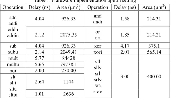
Table 1: Hardware implementation option setting

Operation Delay (ns) Area (µm2) Operation Delay (ns) Area (µm2)

4.04 926.33 and andi 1.58 214.31 add addi addu addiu 2.12 2075.35 _orior 1.85 214.21 4.04 926.33 xor 4.17 375.1 sub subu 2.14 2049.41 xori 2.01 565.14 mult 5.77 84428 multu 5.65 79778.1 nor 2.00 250.00 2.64 1144 slt slti sltu sltiu 1.01 2636 sll sllv srl srlv sra srav 3.00 400.00

In the simulation, we assume that: (1) the CPU core is synthesized in 0.13 µm CMOS technology and executes in 100MHz; (2) the area of the base CPU core, in which no register file is comprised, is 1378855.84µm2; (3) the read/write ports of register file are 2/1, 4/2 and 6/3, respectively; and (4) the execution cycle of all instructions in PISA is one cycle, i.e. 10 (ns). Table 1 lists the hardware implementation option settings (delay and area) of instructions in PISA. Significantly, only instructions that can be grouped into ISEs are listed in table 1. These settings were either obtained from Lindstrom [19], or modeled by Verilog and synthesized with Synopsys Design Compiler. Since enlarging the number of read/write ports in the register file increases the required silicon area, different read/write ports of register file were also synthesized. Therefore, the silicon areas of the CPU cores with 2/1, 4/2 and 6/3 (register file read/write ports) were 1500000µm2, 1574138.80µm2 and 1631359.54µm2, respectively.

Because of the heuristic nature of the ISE exploration algorithm, the exploration was repeated 5 times within each basic block, and the best result among the 5 iterations was chosen.

For obtaining the set of parameters (α, ρ, β1, β2 and β3), this work adopted a

greedy-like method. The parameter exploration method is described as follows: Step 1: Randomly select a smaller basic block, and manually compute its

optimal result. Then, randomly choose a set of parameters. Based on this set of parameters, only adjust one parameter at a time to execute the proposed algorithm. When the simulation result is equal or very close to the optimal one, stop adjusting this parameter and start to adjust other parameters. Once all the parameters are obtained, enter Step 2.

(25)

algorithm to compute their results using the set of parameters obtained in step 1. If the proposed algorithm converges for these bigger basic blocks, apply this set of parameters for all basic blocks. Otherwise, go back to Step 1, and use other smaller basic block to find a set of parameters. If the proposed algorithm can not converge for all basic blocks, go back to Step 1, too.

Note that the basic block(s) used in Step 1 and 2 must be chosen among the result of BB selection in the ISE design flow. The parameters adopted in this paper and their meanings are listed below.

♦ α: the weight of merit and pheromone in px,j.

♦ ρ : the evaporating factor in trail update.

♦ β1: the decay speed when a selected-hardware-implementation-option

operation is stand alone.

♦ β2: the decay speed when the input/output constraint is violated.

♦ β3: the decay speed when the convex constraint is violated.

A large α makes the algorithm converge slowly, while a small α is on the contrary. Restated, a large α obtains a solution slowly, and a small α obtains a poor solution, but quickly. ρ has same characteristic with α. β1, β2 and β3 affect the opportunity of being

selected again for the violated-constraint(s) implementation option. In other words, large β1, β2 and β3 let the violated-constraint(s) implementation option have higher

chance of being selected again at following iterations.

In this experiment, the initial merit value of the software and hardware implementation option was 100 and 200, respectively; P_END was 99%. The probability value adopted α = 0.25, the evaporating factor ρ was 5, and the merit function had β1 = 0.9, β2 = 0.9 and β3 = 0.5.

Additionally, since [author of 3]’s approach [3] does not consider pipestage timing constraint, we assume that it always deploys the fastest implementation option for every operation in ASFU.

4.2 Experimental results

Figures 7 and 8 depict the average execution time reduction and the average extra silicon area cost of Mibench with different numbers of ISE, respectively. Each bar in Figs. 7 and 8, comprises several segments, which indicate the execution time reduction using 1, 2, 4, 8, 16 and 32 ISEs. The first word of each label on X axis in both Figs. 7 and 8 indicates which ISE exploration algorithm is adopted. “Proposed” and “genetic” denote the proposed ISE exploration algorithm and that of [author of 3] [3], respectively. The first and second symbols in parentheses of each label on the X-axis are the number of register file read/write ports in use, and which optimization method (-O0 or -O3) is used. For instance, (4/2, O3) means that the register file has 4

(26)

read ports as well as 2 write ports, and that the -O3 optimization method is employed. For both algorithms, -O3 exhibits better execution time reduction than -O0 in most cases. Possibly, -O3 often uses various compiler optimization techniques. Some of these techniques (like loop unrolling, function inlining, etc.) remove branch instructions, and increase the size of basic block(s). The bigger basic block usually has a larger search space, such that it has a greater opportunity to obtain the ISEs, which consist of more operations. This results in more execution time reduction. However, increasing the size of basic blocks also enlarges the opportunity of violating register read/write port constraint, when only few read/write ports can be used, e.g. 2/1. This is why -O3 has less execution time reduction than -O0 in some cases.

Most of execution time reduction is dominated by several ISEs within hot basic blocks. In other words, the number of ISE is not entirely proportional to the execution time reduction. In most cases, 8 ISEs can perform over half of execution time reduction achieved by 32 ISEs, and only utilize less than quarter of silicon area used by 32 ISEs. For instance, while using 4/2 (register file read/write ports) register file, 8 ISEs can save average 14.95% execution time and cost 81467.5µm2 silicon area, which is 5.43% of the original core area. Conversely, if 32 ISEs are adopted, then the average execution time reduction can rise to 20.62%, but extra area cost also increases to 345135.45µm2, which is 23.01% of the original core area.

0% 5% 10% 15% 20% 25% 30% prop osed ( 2/1, O0) prop osed ( 2/1, O3) gene tic ( 2/1, O0) gene tic ( 2/1, O3) propo sed ( 4/2, O0 ) propo sed (4/2 , O3 ) gene tic ( 4/2, O0) gene tic ( 4/2, O3) propo sed (6/ 3, O 0) prop osed (6/ 3, O 3) gen etic (6 /3, O 0) gen etic (6 /3, O 3) E x ec ut io n T im e R e du c ti o n 1 2 4 8 16 32

(27)

0 100000 200000 300000 400000 500000 600000 700000 propo sed (2 /1, O 0) propo sed (2 /1, O 3) genet ic ( 2/1, O0) genet ic ( 2/1, O3) pro pose d (4 /2, O 0) propo sed (4/2 , O 3) gen etic (4/ 2, O 0) genet ic ( 4/2, O3) propo sed (6/3, O0) propo sed ( 6/3, O3) genet ic ( 6/3 , O 0) genet ic (6 /3, O 3) Ex tr a Ar e a Co s t 1 2 4 8 16 32

Figure 8: Extra silicon area cost

Except for several cases in 6/3 (register file read/write ports), the proposed ISE exploration algorithm achieved a better execution time reduction than [author of 3] [3]. The proposed approach has lower performance improvement in some cases because one set of parameters (α, β1, β2 and β3) does not work well in all cases. This problem

can be mitigated by dynamically adjusting these parameters according to different situations. Theoretically, ISE candidates always adopting the fastest hardware implementation option would have the best performance. However, as revealed in Fig. 7, the proposed ISE exploration algorithm has better execution time reduction in most cases, since even in the same BB, the operations grouped into an ISE candidate and the number of ISE candidate explored by both algorithms may be not identical.

Because the proposed ISE exploration algorithm explores not only ISE candidate but also their implementation options, less extra silicon area is used in all cases. Figure 9 illustrates the silicon area saving of proposed algorithm for all cases, as compared with the genetic algorithm [3]. Obviously, the proposed algorithm can significantly reduce the extra silicon area cost. Figure 9 also reveals that relaxing the constraint of register file read/write ports tends to decrease the silicon area saving. Relaxing the constraint of register file read/write ports can increase the number of operations grouped into ISE. However, the operations grouped into ISE due to relaxing the constraint of register file read/write ports usually are logic operations such that only one hardware implementation option can be selected. This leads to less silicon area being saved using our approach.

(28)

0.00% 10.00% 20.00% 30.00% 40.00% 50.00% 60.00% 70.00% 80.00% 1 2 4 8 16 32 Number of ISE S ili c o n a rea s a v in g

(2/1, O0) (2/1, O3) (4/2, O0) (4/2, O3) (6/3, O0) (6/3, O3)

Figure 9: Silicon area saving

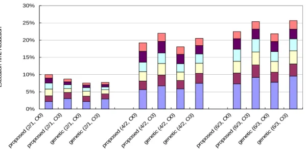
From another perspective, under the same silicon area constraints, adopting the miser implementation option can enlarge the number of ISEs that can be utilized in processor core, can increase the level of performance improvement. Figure 10 shows this perspective. In Fig. 10, each bar consists of several segments, which indicate the execution time reduction under different silicon area constraints, are 5%, 10%, 15%, 20%, 25% and 30% of the original CPU core size. In all cases, the proposed ISE exploration algorithm has better performance improvement than genetic algorithm [3]. Significantly, the improvement in execution time reduction is not in proportion to the available silicon area, since most execution time reduction is dominated by several ISEs. Table 2 presents the detailed results of Fig. 10. describe why only few performance improvement 0% 5% 10% 15% 20% 25% 30% propos ed ( 2/1, O0 ) propos ed ( 2/1, O3 ) genet ic (2 /1, O 0) genet ic (2 /1, O 3) propo sed ( 4/2, O 0) propo sed ( 4/2, O 3) genet ic (4 /2, O 0) genet ic (4 /2, O 3) propos ed (6 /3, O0 ) propos ed (6/3, O3) gene tic (6 /3, O 0) gen etic (6/3, O3 ) E x ec u ti on T im e Reduc ti o n 5% 10% 15% 20% 25% 30%

(29)

Figure 10: Execution time reduction under different silicon area constraint Table 2: Execution time reduction under different silicon area constraint Silicon area

constraint 5% 10% 15% 20% 25% 30%

Number of ISE being selected

proposed (2/1, O0) 13 28 50 71 102 128

proposed (2/1, O3) 12 27 40 55 79 100

genetic (2/1, O0) 8 15 22 35 48 61

genetic (2/1, O3) 8 12 18 26 34 46

Execution time reduction

proposed (2/1, O0) 8.60% 9.81% 10.38% 10.61% 10.76% 10.83% proposed (2/1, O3) 7.57% 8.49% 8.94% 9.29% 9.54% 9.64% genetic (2/1, O0) 6.23% 6.90% 7.25% 7.63% 7.87% 8.01% genetic (2/1, O3) 6.42% 6.83% 7.23% 7.57% 7.79% 8.05%

proposed (4/2, O0) 8 18 23 34 46 56

proposed (4/2, O3) 6 14 20 26 34 45

genetic (4/2, O0) 4 8 14 21 28 36

genetic (4/2, O3) 4 8 14 19 22 26

proposed (6/3, O0) 5 12 19 25 31 39

proposed (6/3, O3) 6 9 14 19 25 32

genetic (6/3, O0) 4 7 12 17 22 28

genetic (6/3, O3) 4 7 10 15 19 23

4.3 Optimal Solution

To understand the quality of ISE candidates explored by the proposed ISE exploration algorithm, the results of proposed algorithm are compared with the optimal solution, as shown in Table 3. Table 4 compares the processing times. The

(30)

legal pattern number is the number of ISE candidates that obey constraints (input/output constraint, convex, no load/store operation). The processing time of the optimal solution strongly depends on the DFG size or legal pattern number. The results of proposed algorithm are very close to the optimal result when the optimal solution can be obtained successfully. Nevertheless, the proposed algorithm can significantly decrease the computing time. Additionally, releasing the input/output constraint normally increases the legal pattern number significantly. In this case, the optimal solution is difficult to obtain, but the proposed algorithm still behaves well.

Table 3: Comparison of optimal solution and ISE Exploration Algorithm (result) Optimal Solution Proposed Algorithm DFG Size Legal Pattern Number In / Out Constraint Cycle Reduction Extra Area Cost Cycle Reduction Extra Area Cost 13 4 2 / 1 3 1228 3 1228 26 9 2 / 1 5 7381 5 7603 20 30 2 / 1 8 11683 6 9152 41 7 2 / 1 7 10028 7 10028 64 1 2 / 1 1 1141 1 1141 32 45 2 / 1 --* -- 16 107160 23 75 2 / 1 -- -- 9 13886 13 2 / 1 5 6454 4 5128 12 28 4 / 2 6 8752 6 8752 13 2 / 1 9 9127 9 9350 46 4 / 2 -- -- 13 13929 44 108 6 / 3 -- -- 15 14357

P.S. *: means the solution can’t be obtained in practical time.

Table 4: Comparison of optimal solution and ISE Exploration Algorithm (processing time)

Optimal Solution Proposed Algorithm DFG Size Legal Pattern Number In / Out Constraint Processing Time Processing Time 13 4 2 / 1 0.01s 0.03s 26 9 2 / 1 0.03s 1.21s 20 30 2 / 1 14m22.46s 2.705s 41 7 2 / 1 2m12.53s 1.249s 64 1 2 / 1 4.08s 0.753s 32 45 2 / 1 --* 4.49s 23 75 2 / 1 -- 2.333s 12 13 2 / 1 0.01s 0.438s

(31)

28 4 / 2 2m15.33s 0.777s

13 2 / 1 4.73s 1.786s

46 4 / 2 -- 2.102s

44

108 6 / 3 -- 3.067s

P.S. *: means the solution can’t be obtained in practical time.

5. 結論

The proposed ISE generation algorithm can significantly reduce the silicon area cost with almost no performance loss. Previous studies in ISE exploration deploy the fastest implementation option for each operation in ASFU to achieve the highest speed-up ratio. Nevertheless, the fastest implementation option is not always the best choice in terms of performance and silicon area cost. This work considers the pipestage timing constraint, such that the proposed ISE exploration algorithm explores not only ISE candidates, but also their implementation option. The advantages of the proposed ISE exploration algorithms are as follows: (1) significantly lower the extra silicon area cost with almost no performance loss, and (2) is polynomial time solvable. Experiment results demonstrate that the proposed design can further decrease the extra silicon area by up to 69.43%, 1.26% and 33.8% (max., min. and avg., respectively), and also has a maximum performance improvement of 1.6%.

Additionally, we recommend addressing several issues in future work. First, the parameters (α, ρ, β1, β2 and β3) significantly influence experimental results. This work

adopts the same set of parameters for different cases, i.e. different combination of register file read/write ports and the size of BB. However, the dynamic adjustment for these parameters to further improve performance would be interesting to study. Second, [combination] raises one interesting issue, namely “ISE combination”. Without introducing any performance loss, if several analogous ISE candidates are merged into one, or one hardware resource is used to execute identical operations in the same ISE, then the silicon area can be further lowered. Third, most ISE exploration algorithms only address on the single-scalar processor, which issues at most a single instruction per cycle into its execution pipeline. Grouping operations into ISE can often benefit in performance improvement in a single-scalar processor. Nevertheless, it would not be true in a multiple-issue processor. Grouping operations, which can be executed in parallel with others in a multiple-issue processor, into ISE is difficulty to improve performance, but increases the silicon area cost. ISE exploration in the multiple-issue processor would be another interesting issue.

(32)

6. 計畫成果自評

在第一年的計畫執行過程中，我們針對嵌入式 embedded processor 在

instruction bus 上的省電需求，提出一同時兼具 register relabeling 以及 instruction encoding 優點的演算法，使編碼後的資料在 instruction bus 上傳送時的 bit toggle 數更小。並針對這個議題發表了三篇碩士論文：(1) 降低傳送次數之窄匯流排編碼[20]、(2) 嵌入式系統低功率指令匯流排編碼方法[21]、(3) 減少嵌入式處理器之程式記憶體的資料匯流排耗電[22]。這些碩士畢業論文針對 instruction bus 上的耗能進行分析並提出相關的演算法。在第二年的計畫時程中，我們更進一步地針對embedded processor 提出兩個減低電源消耗的方法。分別為微處理機之省電設計與低耗電instruction cache。在第二年度的成果中，我們發表了兩篇碩士論文：(1)ARM9 微處理機之省電設計 [23]，與(2)可被窄寬度運算共用之單一管線資料路徑設計[24]，和一篇國際性會議論文，Instruction fetch power reduction using forward-branch bufferable innermost loop bufferp [25]。在第三年的計畫執行中，我們則針對 embedded processor 提出一個增進其執行效能的方法，稱之為延伸指令集(instruction set extension, ISE)。在本年度的中我們發表了一篇碩士論文與一篇國際性會議論文：(1) 考量管線時間之延伸指令集[26]，(2) Instruction set extension generation with considering physical constraints[27]。綜觀為期三年的計畫執行，我們針對 SoC 上省電與效能這兩項議題提出數篇碩士畢業論文與國際性會議論文。其中，在省電這個議題上，我們總共提出了五篇碩士畢業論文；而在效能這個議題上，則分別提出了一篇碩士畢業論文與國際性會議論文。總結來說，在這幾年的研究中，我們不僅僅對於 SoC 上省電與效能這兩項議題上發表具體的研究。對於其他應用的發展亦有具體的成果發表，並期望這些成果對於國內在發展相關產業時能提供具體的助益。

7. 參考資料

[1] T. R. Halfhill, “Tensilica’s software makes hardware,” Microprocessor Report, 23 June 2003.

[2] ——, “ARC Cores encourages “plug-ins”,” Microprocessor Report, 19 June 2000. [3] T. R. Halfhill, “MIPS embraces configurable technology,” Microprocessor

Report, 3 Mar. 2003.

[4] ——, “Altera’s new CPU for FPGAs,” Microprocessor Report, 28 June 2004. [5] M. Dorigo, V. Maniezzo, and A. Colorni, “Ant System: Optimization by a

(33)

Colony of Cooperating Agents,” IEEE Transactions on Systems, Man and Cybernetics, February 1996.

[6] Gang Wang, Wenrui Gong and Ryan Kastner, “Application Partitioning on Programmable Platforms Using the Ant Colony Optimization”, Journal of Embedded Computing, 2006.

[7] Mouloud Koudil, Karima Benatchba, Said Gharout and Nacer Hamani, “Solving Partitioning Problem in Codesign with Ant Colonies,” IWINAC, 2005.

[8] Laura Pozzi, Kubilay Atasu, and Paolo Ienne, “Exact and Approximate Algorithms for the Extension of Embedded Processor Instruction Sets,” IEEE Transactions on Computer Aided Design, July, 2006.

[9] Partha Biswas, Sudarshan Banerjee, Nikil Dutt, Laura Pozzi, and Paolo Ienne, “Fast automated generation of high-quality instruction set extensions for processor customization,” In Proceedings of the 3rd Workshop on Application Specific Processors, September 2004.

[10] Nathan T. Clark, Hongtao Zhong and Scott A. Mahlke, “Automated Custom Instruction Generation for Domain-Specific Processor Acceleration,” IEEE Transactions on Computers, October, 2005.

[11] Pan Yu and Tulika Mitra, “Characterizing embedded applications for instruction-set extensible processors,” DAC, 2004.

[12] Pan Yu and Tulika Mitra “Satisfying real-time constraints with custom instructions,” CODES+ISSS, 2005.

[13] Edson Borin, Felipe Klein, Nahri Moreano, Rodolfo Azevedo, and Guido Araujo. “Fast Instruction Set Customization”, ESTIMedia, September 2004.

[14] Armita Peymandoust, Laura Pozzi, Paolo Ienne, and Giovanni De Micheli, “Automatic Instruction-Set Extension and Utilization for Embedded Processors,” In Proceedings of the 14th International Conference on Application-specific Systems, Architectures and Processors, June 2003.

[15] Jason Cong, Yiping Fan, Guoling Han and Zhiru Zhang, “Application-Specific Instruction Generation for Configurable Processor Architectures,” Twelfth International Symposium on Field Programmable Gate Arrays, 2004.

[16] Samik Das, P. P. Chakrabarti, Pallab Dasgupta, “Instruction-Set-Extension Exploration Using Decomposable Heuristic Search,” VLSI Design, 2006.

[17] T. Austin, E. Larson, and D. Ernst, “SimpleScalar: An infrastructure for computer system modeling,” IEEE Computer, 2002.

[18] M. R. Guthaus, J. S. Ringenberg, D. Ernst, T. M. Austin, T. Mudge and R. B. Brown, “Mibench: A free, commercially representative embedded benchmark suite,” IEEE Annual Workshop on Workload Characterization, 2001.

(34)

http://www.ce.chalmers.se/arithdb/

[20] 鄭式勳, “降低傳送次數之窄匯流排編碼,” 碩士論文

[21] 陳彥銘, “嵌入式系統低功率指令匯流排編碼方法,” 碩士論文

[22] 鄭欽宗, “減少嵌入式處理器之程式記憶體的資料匯流排耗電,” 碩士論文, [23] 蔡佳洲, “ARM9 微處理機之省電設計,” 碩士論文

[24] Bin-Hua Tein, I-Wei Wu, and Chung-Ping Chung, “Instruction fetch power reduction using forward-branch bufferable innermost loop buffer,” International Conference on Computer Design, Las Vegas, Nevada, USA, June 26-29, 2006. [25] 黃士嘉, “考量管線時間之延伸指令集,” 碩士論文

[26] 林聖勳, “可被窄寬度運算共用之單一管線資料路徑設計,” 碩士論文

[27] I-Wei Wu, Shi-Jia Huang, Chung-Ping Chung, and Jyh-Jiun Shann, “Instruction set extension generation with considering physical constraints,” International Conference on High Performance Embedded Architectures & Compilers (HiPEAC), Lecture Notes in Computer Science LNCS 4367, Ghent, BELGIUM, January 28-30, 2007.