微陣列資料的統計型態發掘(III)

行政院國家科學委員會專題研究計畫 成果報告

微陣列資料的統計型態發掘(3/3)

計畫類別： 個別型計畫

計畫編號： NSC93-2118-M-009-001-

執行期間： 93 年 08 月 01 日至 94 年 10 月 31 日

執行單位： 國立交通大學統計學研究所

計畫主持人： 盧鴻興

報告類型： 完整報告

報告附件： 國外研究心得報告

處理方式： 本計畫可公開查詢

中 華 民 國 94 年 10 月 31 日

I

行政院國家科學委員會專題研究計畫成果報告

微陣列資料的統計型態發掘(3/3)

Statistical Pattern Discovery for Microarray Data

計畫編號：NSC 93-2118-M-009-001

執行期限：93 年 8 月 1 日至 94 年 10 月 31 日

主持人：國立交通大學統計學研究所盧鴻興教授

一、中文摘要

針對高效能的微陣列技術中的隨機

性，我們需要應用統計方法來發展微陣列

資料的的型態發掘，用以提供生物學及醫

學研究的深入洞悉。我們這三年的長期計

劃將發展一系列新的統計工具，來分析微

陣列產生的基因表現資料。在進行微陣列

資料探勘與知識發掘工作中，我們將面臨

下列的主要議題。

第一步是選取特徵表示，用來定義基

因微陣列資料的主要特徵型態。對於具有

時間性的資料，多重解析法，例如小波，

可以用來作特徵表示。對於不具時間性的

資料，則可運用不同的距離測度和離散法

來作特徵表示。接著，非線性維度減化的

技巧可以進一步應用來調整距離測度和尋

找資料適合的維度。這些技巧可以整合群

集分析的方法，包含多元尺度法，階層式

群聚法等等，作資料的探索分析。

下一步是進行監督式分類。由於現在

的微陣列資料只有數百個陣列，但卻有超

過數千個基因表現概廓，因此有需要篩檢

或濾除出管家基因或無資訊基因。為了解

決這些分類問題的困難，我們可以整合先

驗訊息和其它相關的資訊到進階的分類法

中，來分類樣本和基因的功能。交叉認証

法可以用來評量這些方法的預測誤差。

最後，在這後基因體世代中，我們還

需要發展新的統計工具，從微陣列資料中

推論基因的反應路徑。針對微陣列資料的

特性，我們將提出新的統計觀點。這些新

的方法將會與現有的方法相比較，找出優

缺點。我們也將同時應用國際和國內研究

團隊所產生的互補 DNA 晶片和寡核甘酸晶

片資料，進行我們的統計研究。

關鍵詞：資料探勘，知識發掘，特徵表示，

多重解析分析，小波，群集分析，非線性

維度減化，分類法，先驗訊息，預測誤差，

交叉認証，反應路徑分析。

Abstract

Due to the inherent randomness in the

high throughput technique of microarray,

pattern discovery by statistical methods are

important to provide insights for biological

and medical studies. This three-year project

is hence aimed at exploring a series of new

statistical tools for analyzing gene expression

data generated by microarray. We will

focus on the following major issues involved

in the tasks of data mining and knowledge

discovery for microarray data.

The first is regarding the feature

representation to define main patterns for

microarray data. For data with time courses,

multiresolution analysis, like wavelets, will

be investigated. For data without time

course, different distance measures and

discretization methods will be studied.

Then, nonlinear dimension reduction

techniques can be further applied to adjust

the distance measures and search for intrinsic

dimension. These techniques can be

integrated with cluster analysis for

exploratory data analysis, including

multidimensional scaling, hierarchical

clustering, and so forth.

II

The next issue is about supervised

classification. Because current microarray

data only have hundred arrays with

expression profiles of more than thousands

genes, it is important to filter or screen

housekeeping or noninformative genes. In

order to solve the ill-posedness of these

classification problems, prior knowledge and

other related information will be

incorporated with advanced classification

methods to classify samples and the function

of genes. Prediction errors by

cross-validation will be studied to evaluate

the performance.

Finally, it is intended to develop new

statistical tools for inferring the pathways

from microarray data in this post-genome era.

New perspectives that emphasis the

particular properties of microarray data will

be addressed. Comparisons of all these new

methods with existing methods will be

performed as well. Both cDNA and

oligonucleotide chips produced in

international and local research groups will

be studied for these methods.

Keywords: Data Mining, Knowledge

Discovery, Feature Representation,

Multiresolution Analysis, Wavelets, Cluster

Analysis, Nonlinear Dimension Reduction,

Classification, Prior Knowledge, Prediction

Error, Cross-Validation, and Pathway

Analysis.

1

二、緣由與目的

The massive amonut of microarray data

bring the big challenge of developing

advanced data mining tools by statistical and

computational methods, which motivate our

great research interests in this three-year

project. In particular, these data are high

dimensional because the sample number is far

smaller than the gene number, which causes

the curse of dimensionality and stimulates the

development of new data analysis methods

(Donoho 2000). Therefore, this long-term

project is aimed to develop new techniques to

analyze microarray data generated by

international and local research laboratories

with state-of-art analysis tools and databases

in the world for statistically pattern

discovery.

Focusing on specific scientific problems,

new data mining and knowledge discovery

techniques will be developed and investigated.

For example, filtering, screening, and

exploratory data analysis of microarray data

will be investigated. Dimension reduction

and visualization techniques will be invented

to extract the genuine feature in these data.

Integration of related databases and

biological knowledge would be performed to

verify and confirm new findings.

Systematical methods for unsupervised

clustering and supervised classification will

be developed.

三、結果與討論

本三年期計畫到目前為止己

完成 9

篇

論文如下。

1. “Rapid divergence in expression between

duplicate genes inferred from microarray

data,” Trends in Genetics, 18, 12, 609-613,

2002.

2. “On Visualization, Screening, and

Classification of Cell Cycle-Regulated Genes

in Yeast,” The 14th International Conference

on Genome Informatics (GIW2003), 344-345,

2003.

3. “Statistical Analysis of the Gene

Expression for Non-synchronized Cell

Cycles of Human Glioma Cells after Gamma

Irradiation by cDNA Microarray,” Technical

Report.

4. "Evolution of the yeast protein interaction

network,"

PNAS (Proceedings of the

National Academy of Sciences of the United

States of America), 100, 22, 12820-12824,

2003.

5. "Gene Expression Analysis Refining

System (GEARS) via Statistical Approach: A

Preliminary Report," The 14th International

Conference on Genome Informatics

(GIW2003), 316-317, 2003.

6. "Supervised Motion Segmentation by

Spatial-Frequential Analysis and Dynamic

Sliced Inverse Regression," Statistica Sinica,

14, 413-430, 2004.

7. “Patterns of Segmental Duplications in the

Human Genome,” Mol. Biol. Evol., 22, 1,

135-141, 2005.

8. “Explore Biological Pathways from Noisy

Array Data by Directed Acyclic Boolean

Networks,”

Journal of Computational

Biology, 12, 2, 170-185, 2005.

9. “Gridding Spot Centers of Smoothly

Distorted Microarray Images,” IEEE

Transactions on Image Processing, accepted.

四、計畫成果自評

由上述的報告中，可以發現我們的研

究內容與原計畫相符，達成預期的目標。

我們將進一步將完成的技術報告投稿到學

術期刊發表，並進一步將這些技術應用到

實際的微陣列資料，提供更正確和有效的

統計分析。因此，本計畫的研究除了在學

術上分析方法的突破，也同時具備應用的

價值。

五、參考文獻

2 decomposition for genome-wide expression data processing and modeling. Proc Natl Acad Sci 2000 Aug 29;97(18):10101-6.

[2] Brown MP, Grundy WN, Lin D, Cristianini N, Sugnet CW, Furey TS, Ares M Jr, Haussler D. Knowledge-based analysis of microarray gene expression data by using support vector machines. Proc Natl Acad Sci 2000 Jan 4;97(1):262-7. [3] Celis JE, Kruhoffer M, Gromova I, Frederiksen C,

Ostergaard M, Thykjaer T, Gromov P, Yu J, Palsdottir H, Magnusson N, Orntoft TF. Gene expression profiling: monitoring transcription and translation products using DNA microarrays and proteomics. FEBS Lett 2000 Aug 25;480(1):2-16. [4] Cheung VG, Morley M, Aguilar F, Massimi A,

Kucherlapati R, Childs G. Making and reading microarrays. Nat Genet 1999 Jan;21(1 Suppl):15-9.

[5] Cho RJ, Campbell MJ, Winzeler EA, Steinmetz L, Conway A, Wodicka L, Wolfsberg TG, Gabrielian AE, Landsman D, Lockhart DJ, Davis RW. A genome-wide transcriptional analysis of the mitotic cell cycle. Mol Cell 1998 Jul;2(1):65-73. [6] Cho RJ, Huang M, Campbell MJ, Dong H,

Steinmetz L, Sapinoso L, Hampton G, Elledge SJ, Davis RW, Lockhart DJ. Transcriptional regulation and function during the human cell cycle. Nat Genet 2001 Jan;27(1):48-54.

[7] Cox TF, Cox MAA. Multidimensional Scaling. 2000 CRC Press, London.

[8] Daubechies I. Ten Lectures on Wavelets. 1992 CBMS-NSF Series of Applied Mathematics, SIAM, Philadelphia.

[9] Donoho DL. High-Dimensional Data Analysis: The Curses and Blessings of Dimensionality. American Math. Society conference: Math Challenges of the 21st Century, Los Angeles, California, August 6-11, 2000.

[10] Duggan DJ, Bittner M, Chen Y, Meltzer P, Trent JM. Expression profiling using cDNA microarrays. Nat Genet 1999 Jan;21(1 Suppl):10-4.

[11] Eisen MB, Spellman PT, Brown PO, Botstein D. Cluster analysis and display of genome-wide expression patterns. Proc Natl Acad Sci 1998 Dec 8;95(25):14863-8.

[12] Eisen MB, Brown PO. DNA arrays for analysis of gene expression. Methods Enzymol 1999;303:179-205.

[13] Friedman N, Nachman I, Pe'er D. Using Bayesian Networks to Analyze Expression Data. ECOMB 2000. The Fourth Annual International Conference on Computational Molecular Biology, Tokyo, Japan.

[14] Halgren RG, Fielden MR, Fong CJ, Zacharewski TR. Assessment of clone identity and sequence fidelity for 1189 IMAGE cDNA clones. Nucleic Acids Res 2001 Jan 15;29(2):582-8.

[15] Hedenfalk I, Duggan D, Chen Y, Radmacher M, Bittner M, Simon R, Meltzer P, Gusterson B, Esteller M, Kallioniemi OP, Wilfond B, Borg A, Trent J. Gene-expression profiles in hereditary breast cancer. N Engl J Med 2001 Feb

22;344(8):539-48.

[16] Kanehisa M. Post-genome Informatics. 1999 Oxford University Press, Oxford.

[17] Khan J, Simon R, Bittner M, Chen Y, Leighton SB, Pohida T, Smith PD, Jiang Y, Gooden GC, Trent JM, Meltzer PS. Gene expression profiling of alveolar rhabdomyosarcoma with cDNA microarrays. Cancer Res 1998 Nov 15;58(22):5009-13.

[18] Knight J. When the chips are down. Nature 2001 Apr 19;410(6831):860-1.

[19] Kohonen T. Self-Organizing Maps. 1997 Second Extended Edition. Springer. New York.

[20] Lipshutz RJ, Fodor SP, Gingeras TR, Lockhart DJ. High density synthetic oligonucleotide arrays. Nat Genet 1999 Jan;21(1 Suppl):20-4.

[21] Lockhart DJ, Dong H, Byrne MC, Follettie MT, Gallo MV, Chee MS, Mittmann M, Wang C, Kobayashi M, Horton H, Brown EL. Expression monitoring by hybridization to high-density oligonucleotide arrays. Nat Biotechnol 1996 Dec;14(13):1675-80.

[22] Lockhart DJ, Winzeler EA. Genomics, gene expression and DNA arrays. Nature 2000 Jun 15;405(6788):827-36.

[23] Mallat SG. A Wavelet Tour of Signal Processing. 1999 Second Edition, Academic Press, San Diego. [24] Raychaudhuri S, Stuart JM, Altman RB. Principal components analysis to summarize microarray experiments: application to sporulation time series. Pac Symp Biocomput 2000;:455-66.

[25] Schena M, Shalon D, Davis RW, Brown PO. Quantitative monitoring of gene expression patterns with a complementary DNA microarray. Science 1995 Oct 20;270(5235):467-70.

[26] Schulze A, Downward J. Analysis of gene expression by microarrays: cell biologist's gold mine or minefield? J Cell Sci 2000 Dec;113 Pt 23:4151-6.

[27] Sherlock G, Hernandez-Boussard T, Kasarskis A, Binkley G, Matese JC, Dwight SS, Kaloper M, Weng S, Jin H, Ball CA, Eisen MB, Spellman PT, Brown PO, Botstein D, Cherry JM. The Stanford Microarray Database. Nucleic Acids Res 2001 Jan 1;29(1):152-5.

[28] Spellman PT, Sherlock G, Zhang MQ, Iyer VR, Anders K, Eisen MB, Brown PO, Botstein D, Futcher B. Comprehensive identification of cell cycle-regulated genes of the yeast Saccharomyces cerevisiae by microarray hybridization. Mol Biol Cell 1998 Dec;9(12):3273-97.

[29] Tamayo P, Slonim D, Mesirov J, Zhu Q, Kitareewan S, Dmitrovsky E, Lander ES, Golub TR. Interpreting patterns of gene expression with self-organizing maps: methods and application to hematopoietic differentiation. Proc Natl Acad Sci 1999 Mar 16;96(6):2907-12.

[30] Tavazoie S, Hughes JD, Campbell MJ, Cho RJ, Church GM. Systematic determination of genetic network architecture. Nat Genet 1999 Jul;22(3):281-5.

3 geometric framework for nonlinear dimensionality reduction. Science 2000 Dec 22;290(5500):2319-23.

[32] Wong WH. Computational Molecular Biology. J. Amer. Statist. Assoc. 2000;95(449):322-6.

[33]

Zhang H, Yu CY, Singer B, Xiong M.

Recursive partitioning for tumor

classification with gene expression

microarray data. Proc Natl Acad Sci 2001

Jun 5;98(12):6730-5.

TRENDS in Genetics Vol.18 No.12 December 2002

http://tig.trends.com 0168-9525/02/$ – see front matter © 2002 Elsevier Science Ltd. All rights reserved. PII: S0168-9525(02)02837-8

609 Research Update

For more than 30 years, expression divergence has been considered as a major reason for retaining duplicated genes in a genome, but how often and how fast duplicate genes diverge in expression has not been studied at the genomic level. Using yeast microarray data, we show that expression divergence between duplicate genes is significantly correlated with their synonymous divergence (K_S) and also with their nonsynonymous divergence (K_A) if K_A≤≤ 0.3. Thus, expression divergence increases with evolutionary time, and K_Ais initially coupled with expression divergence. More interestingly, a large proportion of duplicate genes have diverged quickly in expression and the vast majority of gene pairs eventually become divergent in expression. Indeed, more than 40% of gene pairs show expression divergence even when K_Sis ≤≤0.10, and this proportion becomes >>80% for K_S>> 1.5. Only a small fraction of ancient gene pairs do not show expression divergence. Published online: 01 November 2002 Expression divergence between duplicate genes has long been a subject of great interest to geneticists and evolutionists [1–4]. Indeed, Ohno [2] and others [3,4] had proposed expression divergence as the first step towards the retention of duplicate genes. In the past, however, studies of expression divergence were usually conducted for a limited number of gene families, providing no general picture of the rate of expression

divergence between duplicate genes in a genome. Fortunately, a general picture can now be seen thanks to the advent of microarray gene expression technology (Box 1) and the complete sequences of many genomes. Indeed, using the microarray technology, Ferea et al. [5] showed that rapid change in gene expression can occur in experimental lineages of yeast.

These advances notwithstanding, there remains the difficulty of dating the divergence time between two duplicate genes, which is needed for inferring the rate of expression divergence. In a

pioneering study using microarray data from Saccharomyces cerevisiae, Wagner [6] found no significant correlation

(−0.30, P=0.18) between expression divergence and protein sequence divergence (d) between duplicate genes, and concluded that expression divergence and sequence divergence are decoupled. This result, however, does not imply that expression divergence and evolutionary time are decoupled because d might not be a good proxy of divergence time. Because the rate of amino acid

substitution varies tremendously among proteins [7,8], no single d value can be applied to date the divergence times of different protein or gene pairs. By comparison, the rate of synonymous substitution is more uniform among genes [7,8], and so K_Sis a better proxy of divergence time. We shall therefore rely more on K_Sthan d.

To avoid using correlated data points, we selected independent pairs of duplicate genes in the yeast genome (Box 2).

For each gene family, we started with the pair with the smallest K_Sand continued selecting pairs with increasing K_S, because gene pairs with a small K_Sare fewer than those with a large K_Sand because a smaller K_S can more accurately reflect the time course of expression divergence. Moreover, we selected gene pairs where neither duplicate shows strong codon usage bias, because this bias can retard the increase of K_Sso as to make K_Sa poor proxy of divergence time. Then we analysed the expression divergence for each gene pair using expression data from microarray analyses (see Box 2).

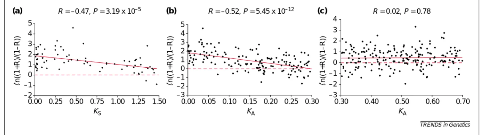
Figure 1a shows a significant negative correlation (−0.47, P<2 ×10−5_{) between} ln[(1+R)/(1−R)] and KS. We used the transformation ln[(1+R)/(1−R)] instead of R to change the scale to a more appropriate one for a linear regression analysis (Box 2); actually, a similar correlation (−0.54) is obtained between R and K_S. A stronger correlation than this is not expected because K_Sis only a crude

Rapid divergence in expression between duplicate genes

inferred from microarray data

Zhenglong Gu, Dan Nicolae, Henry H-S. Lu and Wen-Hsiung Li

A total of 208 cDNA microarray experiment data points were compiled for this study. The dataset represents the gene expression under various developmental and physiological conditions in the yeast life history (Table I).

For some processes, more than one yeast strain or one time course were studied and we randomly selected only one of them for each process. Log₂-transformed ratios of gene expression in experimental populations to reference populations were used in the analysis.

References

a Chu, S. et al. (1998) The transcriptional program of sporulation in budding yeast.

Science 282, 699–705

b Spellman, P.T. et al. (1998) Comprehensive identification of cell cycle-regulated genes of the yeast Saccharomyces cerevisiae by microarray hybridization. Mol. Biol. Cell 9, 3273–3297

c Lyons, T.J. et al. (2000) Genome-wide characterization of the Zap1p zinc-responsive regulon in yeast. Proc. Natl. Acad. Sci. U. S. A. 97, 7957–7962

d Gasch, A.P. et al. (2000) Genomic expression programs in the response of yeast cells to environmental changes. Mol. Biol. Cell 11, 4241–4257

e DeRisi, J.L. et al. (1997) Exploring the metabolic and genetic control of gene expression on a genomic scale. Science 278, 680–686

Box 1. Yeast microarray data

Table I. Studied processes and number of data points in each process

Process Data points Ref. Sporulation 9 [a] Cell cycle 17 [b] Zinc regulation 9 [c] YPD growth 10 [d] Diamide treatment 8 [d] Nitrogen deletion 10 [d] DTT treatment 8 [d] H2O2 treatment 10 [d] Menadione treatment 9 [d]

Diauxic shift 7 [e]

Heat shock 7 [d]

Hyper-osmotic shock 7 [d]

Different carbon resources 6 [d] Amino acid starvation 5 [d] Other experiments in response 86 [d] to environmental changes

proxy of divergence time owing to the considerable variation in synonymous rate among genes [7,8]. As in [6], only a weak correlation (−0.30, P=4.57×10−9₎ is found between ln[(1+R)/(1−R)] and K_A (K_A≤0.70); the correlation is significant because the dataset used is much larger than that in [6]. The weak correlation is not surprising because K_Ais not a good proxy of divergence time, so that no correlation between R and K_Ais expected when K_Abecomes large. Indeed, Fig. 1c shows no correlation (0.02, P=0.77) between ln[(1+R)/(1−R)] and K_Afor K_A>0.30. However, a significant negative

correlation (−0.52) between the two quantities is seen for K_A≤0.30 (Fig. 1b). The range of K_A≤0.30 is somewhat arbitrary, but the correlation coefficient varies only from −0.49 for KA≤0.25 to –0.48 for K_A≤0.35. Thus, expression divergence and K_Aare initially coupled to some extent. The same conclusions hold for Affymetrix microarray data, for which cross hybridization between duplicate genes is a less serious problem (see Supplementary Figure at http://download.bmn.com/supp/tig/ decemberAffymetrix.pdf); the dataset is smaller than cDNA microarray data,

so it was not used in the other analyses in this study.

In the above analysis, all experiments were considered together; that is, R was calculated over all data points. This pooling of data might obscure the relationship between expression divergence and sequence divergence because a pair of duplicate genes are not necessarily involved in all of the

physiological processes tested. Note that if a gene pair is not involved in a process, it is unlikely to evolve expression

divergence in that process. For this reason we now consider R separately for each of TRENDS in Genetics Vol.18 No.12 December 2002

http://tig.trends.com

610 Research Update

Open reading frames in the yeast genome (SGD, http://genome-www.stanford.edu/Saccharomyces/) were grouped into different gene families using a rigorous method [a]. Protein sequences of duplicate genes were aligned using ClustalW [b] and the corresponding coding regions were then aligned based on the protein alignment. The numbers of substitutions per synonymous site (K_S) and per nonsynonymous (K_A) site between duplicate genes were estimated using PAML [c] with default parameters. We selected only gene pairs with K_S≤1.5 because when K_Sbecomes larger it is difficult to obtain a reliable estimate, owing to repeated substitutions at the same site. Similarly, we restricted K_Ato≤0.70. The computer program CodonW (ftp://molbiol.ox.ac.uk/ cu/codonW.tar.Z) was used to calculate the effective number of codons (ENC) for each gene studied.

Duplicate gene pairs were selected as follows: within each gene family, starting from the pair with the smallest K_Sof greater than 0.01, we selected independent gene pairs; that is, pairs that share no genes in common with other pairs. To avoid gene pairs with strong codon usage bias, both genes in a selected pair must have an ENC >35. Our study [a] suggests that K_Sis substantially reduced by codon usage bias when ENC<32, but is only mildly affected when ENC >35. In total, 400 duplicate gene pairs were selected.

Because all of the duplicate gene pairs encoding ribosomal proteins have strong codon usage bias, we consider the divergence in the flanking sequences instead of K_S. For each gene pair, the 200 bp of both upstream and downstream flanking regions of both genes were extracted from gene annotation data. ClustalW was used to do the alignment, followed by minor manual adjustments. Genetic distances were calculated using Tamura and Nei’s six-parameter method [d]. The average of the genetic distances in upstream and downstream flanking regions is denoted as D_flank

(Supplementary Table 2 at http://download.bmn.com/supp/tig/ decemberTable2.pdf).

The Pearson correlation coefficient (R) of gene expression over all data points in Table I in Box 1 was calculated for each selected gene pair if the expression data were available for more than half of the

experiments studied for that pair (396 pairs were calculated, Supplementary Table 3 at http://download.bmn.com/supp/tig/

decemberTable3.pdf). Linear regression analysis was used to investigate the relationship between R and K_S(K_A). Because R is bounded by –1 and 1, the transformation _ln((1+R)/(1−R)) was used and the normal linear regression was then carried out between each pair of K_S(K_A) and the transformed R. The statistical package of S+ was used.

Each of the first 9 processes listed in Table I of Box 1, each of which has eight or more data points, was also treated separately; for each process the Pearson correlation coefficient was calculated for each selected gene pair (Supplementary Table 3 at

http://download.bmn.com/supp/tig/decemberTable3.pdf).

References

a Gu, Z. et al. (2002) Extent of gene duplication in the genomes of Drosophila, nematode, and yeast. Mol. Biol. Evol. 19, 256–262

b Thompson, J.D. et al. (1994) CLUSTAL W: improving the sensitivity of progressive multiple sequence alignment through sequence weighting, position-specific gap penalties and weight matrix choice. Nucleic Acids Res. 22, 4673–4680

c Yang, Z. and Nielsen, R. (2000) Estimating synonymous and nonsynonymous substitution rates under realistic evolutionary models. Mol. Biol. Evol. 17, 32–43 d Tamura, K. and Nei, M. (1993) Estimation of the number of nucleotide

substitutions in the control region of mitochondrial DNA in humans and chimpanzees. Mol. Biol. Evol. 10, 512–526

Box 2. Duplicate gene selection and linear regression analysis

TRENDS in Genetics –2 –1 0 1 2 3 4 5 0.00 0.25 0.50 0.75 1.00 1.25 1.50 KS KA KA R = –0.47, P = 3.19 x 10–5 _{R = –0.52, P = 5.45 x 10}–12 (a) –3 –2 –1 0 1 2 3 4 5 0.00 0.05 0.10 0.15 0.20 0.25 0.30 –3 –2 –1 0 1 2 3 4 0.30 0.40 0.50 0.60 0.70 R = 0.02, P = 0.78 n((1+R)/(1 – R)) (b) (c) n((1+R)/(1 – R)) n((1+R)/(1 – R))

Fig. 1. Relationship between the correlation coefficient (R) of gene expression over all available data points and K_S(K_A) between duplicate genes. (a) A significant negative correlation between ln[(1+R)/(1−R)] and K_Sfor gene pairs with K_S<1.5. (b) A significant negative correlation between ln[(1+R)/(1−R)] and K_Afor gene pairs with K_A≤0.3. (c) No correlation between ln[(1+R)/(1−R)] and K_Afor gene pairs with K_A>0.3.

the first nine tests in Box 1, each of which has eight or more time points.

To define ‘expression divergence’, we note that the correlation coefficient between two duplicate genes is initially 1, so we consider a value of 0.5 as sufficiently low. Note that for R=0.5, R2_{is only 0.25,} so that knowing the pattern of expression of one gene provides little information for predicting the expression pattern of the other gene. More importantly, we actually define ‘expression divergence’ by requiring that the probability of observing the two smallest R values among the nine processes is <0.05, given that the

population (true) correlation coefficient (ρ) is 0.5; see Box 3 for the test method. This definition is likely to underestimate the true degree of divergence because it uses

only the information of two smallest R values in the observed R values and because it assumes that the gene pair is involved in all of the nine processes studied. Indeed, this definition is stringent because, in effect, it requires at least one or two negative R values among the nine processes (Table 1). For example, only 38% of the cases with one negative R show ‘expression divergence’. Moreover, none of the 54 pairs of duplicated

ribosomal protein genes in the yeast genome is ‘divergent’ under this criterion (data not shown).

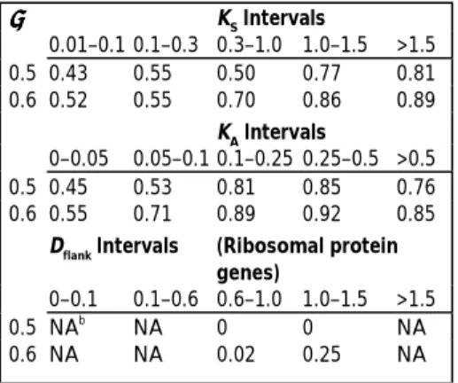
Table 2 shows that over 40% of the non-ribosomal protein gene pairs studied show divergent expression even when K_S≤0.10 and the proportion becomes >80% when KSbecomes larger than 1.5.

The proportion of pairs with diverged expression increases even more rapidly with K_A(Table 2). Clearly, expression divergence has occurred quickly in many of the gene pairs studied.

If we relax the definition of ‘divergent expression’ by setting ρ =0.6 instead of 0.5, the proportion of pairs with divergent expression increases with K_Sat an even faster rate (Table 2). Indeed, more than 50% of the pairs studied show divergent expression even when K_Sis ~0.10. The synonymous rate is not known in yeast but is probably higher than that in Drosophila, which has been commonly taken as 15.6 × 10−9_{nucleotide substitutions per} site per year [7]. Thus, K_S= 0.1 would correspond to less than 3.2 million years of divergence time, implying a rapid rate of TRENDS in Genetics Vol.18 No.12 December 2002

http://tig.trends.com

611 Research Update

For each process under study, denote the n pairs of observations on the expression levels of the two duplicate genes compared by Z = {z_i:i = 1, …, n, and z_I= (x_i,y_i)t_{}. From the sample, the correlation coefficient (R)} between x and y is calculated. We will assume that these n pairs of observations are independently, identically distributed as a bivariate normal distribution with a correlation coefficient (ρ) in the population. This assumption of normality has been checked by the Kolmogorov–Smirnov test on the Q–Q plot for

tanh–1_{(R ) = {ln[(1+R)/(1-R)]}/2 in every process (Supplementary Table 4} at http://download.bmn.com/supp/tig/decemberTable4.pdf).

With a large sample size n, the distribution of R can be approximated as follows. We transform R and ρto tanh–1_{(R) = {ln[(1+R)/(1-R)]}/2 and} tanh–1₍ρ_{) = {ln[(1+}ρ_)/(1-ρ_{)]}/2. Then, the difference tanh}–1_(R) −_tanh–1₍ρ_{) is} approximately a normal variate with the following mean and variance (Ref. [a] p. 433):

mean = ,

variance =

Using this normal approximation, we can evaluate various probabilities. For example, for –1 ≤ c ≤ 1, we can compute

P (cρ,n} = P {R≤ cρ,n} = P {tanh–1_{(R ) ≤ tanh}–1_(c)ρ_,n}

=P {[tanh–1_{(R) – tanh}–1_{(ρ) – u] / σ ≤ [tanh}–1_{(c) – tanh}–1_{(ρ) – u] / σρ,n}}

≈P {Z≤ [tanh–1_{(c) – tanh}–1₍ρ_{) – u] /} σ}

where Z has a standard normal distribution, which can be easily

evaluated.

For a small n, the parametric bootstrap can be used to find out the distribution of R [b]. The mean and variance in the population are estimated by the mean and variance in the sample, which are denoted as

and _.

Given the population correlation coefficient ρ, a bootstrap sample,

Z * = {z*_i:i = 1, …, n}, is obtained by simulating a bivariate normal

distribution with and _.

The correlation coefficient from the bootstrap sample Z * is computed

and denoted as R*. Repeating the resampling procedure B times, we observe R*₁, …, R*B. The empirical distribution of R*1, …, R*Bis used to approximate the distribution of R. In particular,

P (cρ,n) = P (R≤ cρ,n) ,

where I{·} is a indicator function whose value is 1 when the event is true and 0 otherwise. Because the data contain small sample sizes, we will use this parametric bootstrap to estimate probabilities.

Now suppose that m processes are studied and there are njpairs of observations for each process, j = 1, …, m. From the above

approximation, we can evaluate the probability of P_j(c) = P (cρ,n_j}. Then, we can find out the probability that there are κR values observed among the m processes that are ≤c:

P {no R≤ cρ,m} = , P {only one R≤ cρ,m} =

, P {at least two R values ≤ cρ,m} = 1 – P {no R≤ cρ,m} –

P {only one R≤cρ,m} = Eqn [1]

and so forth.

Once we observe the sample correlation coefficients (R values) of one gene pair in the m processes, we can use this parametric bootstrap to evaluate the probability of observing the smallest R values given the population correlation coefficient (ρ). For example, let the smallest two R values be c₁and c₂with c₁≥c₂Then, we can replace c by c₁in Eqn [1]. Of course, by using the complete information of c1and c2, we can obtain a more precise probability:

P {at least one R≤ c₁and one R ≤ c₂ρ,m}

=1 –P {no R≤ c₂ρ,m} – P {only one R≤ c₂and all other R values >c₁ρ,m} Eqn [2]

Note that Eqn [2] is always smaller than or equal to Eqn [1] with c = c₁. All the probability computations in this paper were obtained using Eqn [2].

References

a Rao, C.R. (1973). Linear Statistical Inference and Its Application (2nd Edn), Wiley

b Efron, B. and Tibshirani, R.J. (1998). An introduction to the Bootstrap, Chapman & Hall/CRC

∏

∏

∑

= = = − − − − − = m k k m j m j j j j P c c P c P c P 1 1 1 1 1 2 2 [1 ( )] ) ( 1 ) ( )] ( 1 [ 1

∏

∏

∑

= = = − − − − − m k k m j m j j j j P c c P c P c P 1 1 1 )] ( 1 [ ) ( 1 ) ( )] ( 1 [ 1

∏

∑

∑

∏

= = = ≠ = − = − − m k k m j j j m j m j k k k j P c c P c P c P c P 1 1 1 1 )] ( 1 [ ) ( 1 ) ( )] ( 1 [ ) ( )] ( 1 [ 1 c P m j j

∏

= − B / } { I * 1 c Ri B i ≤ ≈

∑

=     2 2 y y x y x x S S S S S S ρ ρ       y x     2 2 y y x y x x S S RS S RS S       y x 3 1 1) ( 2 4 1 1 2 2 2 − ≈ − − + − = n n n ρ σ ) 1 ( 2 − = n ρ µ

expression divergence between duplicate genes in yeast. A similar picture is seen for K_A(Table 2).

There are two factors that tend to underestimate the rate of expression divergence. First, the nine processes studied do not represent all the physiological processes in yeast, and a duplicate gene pair could have diverged in one or more of the processes that have not been studied, although it has not diverged in any of the nine processes tested. This factor is likely to have significantly reduced our estimate of the rate of expression divergence. Second, there is the possibility of cross-hybridization of cDNA probes when two duplicate genes are highly similar in their cDNA sequences. In view of the fact that many of the highly similar duplicate pairs (K_S<0.10) have shown one or more small R values (data not shown), the extent of cross-hybridization was probably not serious. However, if it were not negligible, the initial rate of expression divergence would have been underestimated.

Alternatively, the noisiness of microarray data tends to reduce the true

correlation (R) between the expression levels of duplicate genes and thus tends to overestimate the rate of expression divergence, especially in the early stage of divergence between duplicate genes. Thus, although our definition of

expression divergence seems stringent for the case of ρ = 0.5, the conclusion should be taken with caution.

It is worth noting that a divergent duplicate pair that has a large K_Sor K_A might already have gained expression divergence when its K_Sor K_Awas still small. Thus, a divergent pair with a large K_Sor K_Adoes not imply a slow rate of expression divergence. It is also interesting to note from Table 2 that the proportion of divergent duplicate gene pairs eventually becomes more than 80% as K_Sincreases. As noted, we have considered only nine processes. If many more processes are considered, the vast majority of duplicate genes will probably eventually become diverged in expression.

There are, however, duplicate genes that do not show divergent expression even when K_Sis large; for example, genes encoding proteasome components, aminopeptidases, aldo/keto reductases and ribosomal proteins. Ribosomal protein genes have not been included in Fig. 1 and Table 1, and have been treated separately in Table 2, because they have strong codon usage bias and their K_Sdoes not reflect the divergence time well. We therefore consider instead the sequence divergence (D_flank) in their flanking regions (Box 2). Note that none of the ribosomal protein gene pairs shows expression divergence under the condition of ρ =0.5 (Table 2). Even under the condition of ρ =0.6, their rate of expression divergence is very slow, compared with that for genes encoding non-ribosomal proteins.

We have examined the functions of quickly diverged gene pairs, that is, those pairs that have a K_S<0.3 but show expression divergence (Supplementary

Table 1 at http://download.bmn.com/ supp/tig/decemberTable1.pdf). The functions of many of these genes are still unknown or have not been well studied. However, we can see that these genes include many membrane proteins such as substrate transporters, and many enzymes such as aldehyde hydrogenase, aldo/keto reductase, helicase and phosphopyruvate hydratase.

In conclusion, because protein distance (or K_A) is not a good measure of divergence time, it was not surprising that no coupling of expression divergence and protein distance was found previously. However, an initial coupling of expression divergence and K_Adoes exist (Fig. 1b). K_Sis a better measure of divergence time than K_A, and the significant correlation of expression divergence with K_Ssuggests that expression divergence increases with divergence time. Most interestingly, many duplicate genes in yeast have diverged quickly in expression and the vast

majority of duplicate genes will eventually become diverged in expression. However, the rate of expression divergence varies among duplicate genes. The majority of duplicate genes such as many membrane proteins and many enzymes have diverged quickly in expression, whereas ribosomal proteins, proteasome

components and some other proteins show a slow rate of expression divergence. Other duplicate genes show a moderate rate of expression divergence. Clearly, a proper analysis of microarray data can shed much light on the rate and mode of expression divergence of duplicate genes. Acknowledgements

We thank Z. Zhu, T. Oakley, M. Long, C-C. Shih, H. Kaessmann, K. Makova, and L. Mets for help and comments. This study was supported by NIH grants.

References

1 Markert, C.L. (1964) Cellular differentiation – an expression of differential gene function. In Congenital Malformations, pp163–174, International Medical Congress

2 Ohno, S. (1970) Evolution by Gene Duplication, Springer-Verlag

3 Ferris, S.D. and Whitt, G.S. (1979) Evolution of the differential regulation of duplicate genes after polyploidization. J. Mol. Evol. 12, 267–317 4 Force, A. et al. (1999) Preservation of duplicate

genes by complementary, degenerative mutations. Genetics 151, 1531–1545 5 Ferea, T.L. et al. (1999) Systematic changes in

gene expression patterns following adaptive evolution in yeast. Proc. Natl. Acad. Sci. U. S. A. 96, 9721–9726

TRENDS in Genetics Vol.18 No.12 December 2002

http://tig.trends.com

612 Research Update

Table 1. Numbers and proportions of gene pairs with expression divergence

(i.e. P < 0.05) for different numbers of negative R values in the nine processes studied.

Number of R Number of gene Gene pairs with P <<<< 0.05a

% Gene pairs with P <<<< 0.05a values pairs ρρρρ= = = = 0.5 ρρρρ= = = = 0.6 ρρρρ= = = = 0.5 ρρρρ= = = = 0.6 0 43 0 0 0 0 1 66 25 49 38% 74% 2 70 61 70 87% 100% ≥3 217 217 217 100% 100% a

The ρ value is the criterion for ‘expression divergence’.

Table 2. Proportion of gene pairs with expression divergencea in different K_S and K_A intervals. ρρρρ K_S Intervals 0.01–0.1 0.1–0.3 0.3–1.0 1.0–1.5 >1.5 0.5 0.43 0.55 0.50 0.77 0.81 0.6 0.52 0.55 0.70 0.86 0.89 K_A Intervals 0–0.05 0.05–0.1 0.1–0.25 0.25–0.5 >0.5 0.5 0.45 0.53 0.81 0.85 0.76 0.6 0.55 0.71 0.89 0.92 0.85

D_flank Intervals (Ribosomal protein genes) 0–0.1 0.1–0.6 0.6–1.0 1.0–1.5 >1.5 0.5 NAb NA 0 0 NA 0.6 NA NA 0.02 0.25 NA a

The criterion for expression divergence is that the probability of observing the two smallest R values in the nine tests studied is less than 0.05, given the population correlation coefficient is ρ. b

TRENDS in Genetics Vol.18 No.12 December 2002

http://tig.trends.com 0168-9525/02/$ – see front matter © 2002 Elsevier Science Ltd. All rights reserved. PII: S0168-9525(02)02820-2

613 Research Update

Techniques & Applications

The detection of single nucleotide polymorphisms by PCR is necessary for many types of genetic analysis, from mapping genomes to tracking specific mutations. This technique is most commonly used when polymorphisms alter restriction endonuclease recognition sites. Here we describe a web-based program, dCAPS Finder 2.0, that facilitates the design of mismatched PCR primers to create or remove a restriction endonuclease recognition site relative to the polymorphism being analyzed.

Published online: 01 November 2002 Molecular genetic research relies heavily on the ability to detect polymorphisms in DNA. These molecular markers range from large deletions and rearrangements to single nucleotide polymorphisms (SNPs) [1]. Before the advent of polymerase chain reaction (PCR) technology [2], restriction fragment length polymorphism (RFLP) analysis required Southern blots of restricted genomic DNA [3]. PCR technology has led to a more rapid, less expensive version of RFLP analysis using cleaved amplified polymorphic sequence (CAPS) markers [4]. However, both RFLP and CAPS analysis require that the SNP creates or removes a restriction endonuclease recognition site. Because this is not always the case, a variety of techniques have been developed to genotype SNPs in an enzyme-independent manner [1]. Many of these techniques require specialized detection equipment and/or labeled PCR primers that cost more than standard

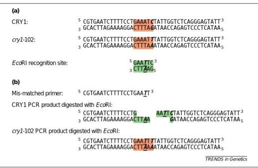
primers. Derived cleaved amplified polymorphic sequence (dCAPS) analysis, widely used in the plant molecular genetics community, uses mismatches in one of the two PCR primers flanking the SNP to create or remove a restriction endonuclease recognition site in one of the two haplotypes being assayed [5,6] (Fig. 1). In this paper, we present a web-based program, dCAPS Finder 2.0, that facilitates the design of these dCAPS primers.

dCAPS Finder 2.0

The dCAPS marker technique was originally developed as a method for

changing a SNP into an RFLP (see [5,6] and references within) (Fig. 1). The technique can also be used to modify an existing RFLP such that a less expensive restriction endonuclease can be used for SNP analysis. Because dCAPS primers use the same chemistry as regular PCR primers, there is also a cost advantage of this technique over more sophisticated, enzyme-independent methods of SNP analysis. The biggest difficulty for designing dCAPS primers lies in identifying restriction endonuclease recognition sites and accompanying primer mismatches. To facilitate this technique, a Macintosh-based computer

Web-based primer design for single nucleotide

polymorphism analysis

Michael M. Neff, Edward Turk and Michael Kalishman

6 Wagner, A. (2000) Decoupled evolution of coding region and mRNA expression patterns after gene duplication: implications for the

neutralist-selectionist debate. Proc. Natl. Acad.

Sci. U. S. A. 97, 6579–6584

7 Li, W-H. (1997) Molecular Evolution, Sinauer Associates

8 Makalowski, W. and Boguski, M.S. (1998) Evolutionary parameters of the transcribed mammalian genome: an analysis of 2,820

orthologous rodent and human sequences.

Proc. Natl. Acad. Sci. U. S. A. 95, 9407–9412

Zhenglong Gu Wen-Hsiung Li*

Dept of Ecology and Evolution, University of Chicago, 1101 East 57th Street, Chicago, IL 60637, USA.

*e-mail: [email protected]

Dan Nicolae

Dept of Statistics, University of Chicago, 5734 S. University Ave, Chicago, IL 60637, USA. Henry H-S. Lu

Insitute of Statistics, National Chiao Tung University, 1001 Ta Hsueh Rd, Hsingchu, 30050 Taiwan.

TRENDS in Genetics

(a)

CRY1: 5′_{CGTGAATCTTTTCCTGAAATCTATTGGTCTCAGGGAGTATT}3′

3′GCACTTAGAAAAGGACTTTAGATAACCAGAGTCCCTCATAA5′

cry1-102: 5′CGTGAATCTTTTCCTGAAATTTATTGGTCTCAGGGAGTATT3′

3′GCACTTAGAAAAGGACTTTAAATAACCAGAGTCCCTCATAA5′

EcoRI recognition site: 5′_{GAA T TC}3′

3′CTT A AG5′

(b)

Mis-matched primer: 5′CGTGAATCTTTTCCTGAA T T3′

CRY1 PCR product digested with EcoRI:

5′_{CGTGAATCTTTTCCTG AA T TCTATTGGTCTCAGGGAGTATT}3′ 3′GCACTTAGAAAAGGACTT A A GATAACCAGAGTCCCTCATAA5′ cry1-102 PCR product digested with EcoRI:

5′_{CGTGAATCTTTTCCTGAA T TTTATTGGTCTCAGGGAGTATT}3′ 3′GCACTTAGAAAAGGACTT A AAATAACCAGAGTCCCTCATAA5′

Fig. 1. Derived cleaved amplified polymorphic sequence (dCAPS) analysis uses a mismatched PCR primer to create

a restriction fragment length polymorphism (RFLP) based on the single nucleotide polymorphism (SNP) being analyzed. (a) The cry1-102 SNP (bold, italic letters) does not create an EcoRI-based RFLP because of one mismatch in the EcoRI recognition site (bold, underlined letters). (b) A primer containing this mismatch (bold, underlined letter) allows the amplification of PCR products that generate an EcoRI -based RFLP that is dependent on the cry1-102 SNP. Red boxes show sequences that are not cleaved by EcoRI. Green boxes represent sequences that are cleaved by EcoRI.

Evolution of the yeast protein interaction network

Hong Qin†_{, Henry H. S. Lu}‡_{, Wei B. Wu}§_{, and Wen-Hsiung Li}†¶

†_{Department of Ecology and Evolution, University of Chicago, 1101 East 57th Street, Chicago, IL 60637;}‡_{Institute of Statistics, National Chiao Tung} University, 1001 Ta Hsueh Road, Hsinchu, Taiwan 30050, Republic of China; and§_{Department of Statistics, University of Chicago, 5734 South} University Avenue, Chicago, IL 60637

Contributed by Wen-Hsiung Li, August 29, 2003

To study the evolution of the yeast protein interaction network, we first classified yeast proteins by their evolutionary histories into isotemporal categories, then analyzed the interaction tendencies within and between the categories, and finally reconstructed the main growth path. We found that two proteins tend to interact with each other if they are in the same or similar categories, but tended to avoid each other otherwise, and that network evolution mirrors the universal tree of life. These observations suggest synergistic selection during network evolution and provide in-sights into the hierarchical modularity of cellular networks.

B

iological networks are the basis of cellular functions (1, 2). Understanding network evolution may shed light on the hierarchical modularity, scale-free property, and various uses of the building blocks of biological networks (3–12). The yeast protein interaction network is one of the best annotated complex networks to date (13–17). Previous studies on the evolution of this network focused either on gene duplication and molecular evolution at the protein level (9, 10) or on the global statistical properties (12). Neither approach can delineate the network evolutionary path, and there is no other comparable protein interaction data for the system-level comparison approach (5). Therefore, uncovering the growth patterns and the evolutionary path of the protein interaction network is a serious challenge (3, 4, 6, 7, 9, 12).

Parts of the present yeast protein interaction network would have been inherited from the last common ancestor of the three domains of life: Eubacteria, Archaea, and Eukaryotes. Thus, an analysis of the evolution of the yeast protein interaction network may provide new insights into the origin of eukaryotic cells (18–21), which has been a controversial issue.

A key question in the evolution of biological complexity (6, 7, 9, 12, 21, 22) is, how have integrated biological systems evolved? Darwinists (21, 23) proposed natural selection as the driving force of evolution. However, the striking similarities between biological and nonbiological complexities have led to the argu-ment that a set of universal (or ahistorical) rules account for the formation of all complexities (22, 24, 25). The yeast protein interaction network is an example of a complex biological system and contributes to the complexity at the cellular level (26). By analyzing the growth pattern and reconstructing the evolution-ary path of the yeast protein interaction network, we can address whether or not network growth is contingent on evolutionary history, which is the key disagreement between the Darwinian view and the universality view (22, 23, 27).

In this article, we studied how the yeast protein interaction network has evolved. We used graph theory to model the yeast protein interaction network. Each yeast protein is a node in the graph. Each pairwise interaction is a link between two nodes. Evolution of the yeast protein interaction network can then be inferred by analyzing the growth pattern of the graph. We classified all of the nodes (proteins) into isotemporal categories based on each protein’s orthologous hits in several groups of genomes that are informative for yeast’s evolutionary history. This scheme gives each protein a binary (b) value representing its evolutionary history. Proteins from the same isotemporal category share similar evolutionary histories. We then analyzed the interaction patterns within and between these isotemporal

categories. Finally, we inferred the main path of the network evolution from six major isotemporal categories.

Materials and Methods

Data Collection.Genomic information of Saccharomyces cerevisiae

was downloaded from the Saccharomyces Genome Database (ftp:兾兾genome-ftp.stanford.edu兾pub兾yeast兾data㛭download) on August 13, 2002. Protein interaction data were obtained from the Comprehensive Yeast Genome Database at the Munich Infor-mation Center for Protein Sequences (MIPS) (http:兾兾 mips.gsf.de兾proj兾yeast兾CYGD兾db兾index.html) (28, 29) on May 28, 2002, and from the reliable subsets of data from high-throughput screens (30). We excluded self-interactions and those involving mitochondrion proteins. The combined data set con-tains 6,633 interaction pairs. Orthologous analyses of the anno-tated ORFs in the yeast genome were parsed out from the clusters of orthologous groups (COGs) of proteins (ftp:兾兾 ftp.ncbi.nih.gov兾pub兾COG) (31, 32) and the published ortholo-gous analysis from the Bork group at the European Molecular Biology Laboratory (EMBL) (30). Mitochondrion genes and a few inconsistent orthologous assignments were removed from the analysis.

Data Analysis. Protein interaction networks were treated as

undirected graphs in adjacency list format (33). Permutations of the networks were carried out in the Chiba City Linux cluster in the Mathematics and Computer Science Division of Argonne National Laboratory (www.mcs.anl.gov兾chiba). Presentation of the network was performed by the program PAJEK (http:兾兾

vlado.fmf.uni-lj.si兾pub兾networks兾pajek) (34). Distance matrix-based analyses were conducted in theRenvironment for

statis-tical computing and graphics (www.r-project.org) (35). The neighbor-joining (NJ) tree was generated by PAUP* (http:兾兾

paup.csit.fsu.edu) and presented by the program TREEVIEW

(http:兾兾taxonomy.zoology.gla.ac.uk兾rod兾treeview.html) (36).

Statistical Analysis of Interaction and Traversal Patterns.To evaluate

the interaction tendencies within and between isotemporal categories, we measured the deviation of each observed inter-action frequency from its random expectation (37). The ob-served interaction frequency between categories i and j, F(i,j)obs, is

compared with the mean interaction frequency, F(i,j)mean, of a series

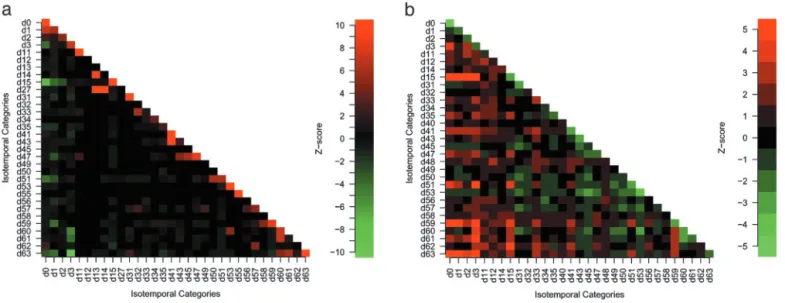
of null models in which all proteins have the same connectivities, but their interaction partners are randomly chosen (37) [termed the Maslov–Sneppen 2002 (MS02) null models]. To describe the deviations of the observed interaction frequencies from the random expectations, we used Z scores, Z(i,j)⫽ [F(i,j)obs ⫺ F(i,j)mean]兾

␴(i,j), where␴(i,j)is the SD of the interaction frequency between

categories i and j in the MS02 null models.

Similarly, we used the Z scores to measure the deviation of the average shortest path between two isotemporal categories from the mean of a series of isomorphic MS02 null models. This

Abbreviations: MS02 null model, Maslov-Sneppen 2002 null model; NJ, neighbor-joining; b, binary; d, decimal.

¶_{To whom correspondence should be addressed. E-mail: [email protected].}

© 2003 by The National Academy of Sciences of the USA

isomorphic MS02 null model retained the same topology with the original network. Network topology can greatly influence the average shortest path. The MS02 null model could change the total number of connected components in the original network and gave uninterpretable Z scores. The isomorphic null model was a simple method to exclude the topological influence on traversal path, and it enabled us to evaluate the association significance between two isotemporal categories.

Network Null Models.To generate an MS02 null model (37), the

original network was first converted to pairwise-interacting nodes. These pairwise interacting nodes were then converted into an array of symbols. Permutation of this array of symbols was then used to generate a new list of pairwise-interacting nodes (self-pairing was prohibited during the permutation), which was then used to generate an MS02 null model in adjacency list format.

To generate an isomorphic MS02 null model, nodes with the same connectivity were concatenated into arrays of symbols. Permutation was then conducted on the arrays of symbols for each connectivity value. The original and the permutated arrays of symbols were then used to generate a lookup table in which each original node corresponded to a new node with the same connectivity. Based on this lookup table, all of the nodes in the original network were then replaced by the new nodes, resulting in a permutated network with the same topology.

Calculation of Average Shortest Path. We slightly modified the

Dijkstra’s algorithm to compute the shortest path (33). For a protein in isotemporal category i, its shortest path to isotemporal category j is defined as its traversal distance to the nearest neighbor in category j. The mean of the shortest paths to category j of all proteins in category i is taken as the distance from i to j, denoted as di3j. Distance from j to i, dj3i, is calculated

similarly. The average shortest path between categories i and j is the average of di3j and dj3i.

Results

Isotemporal Classification of Proteins.To study the growth of the

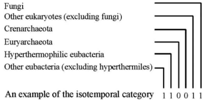
yeast protein interaction network, we classified all yeast proteins into isotemporal categories, based on the presence or absence of their orthologous hits in each of the six groups of the universal tree of life (38), namely hyperthermophilic eubacteria, other eubacteria (excluding the hyperthermophiles), euryarchaeota, crenarchaeota, fungi, and other eukaryotes (excluding fungi) (Fig. 1). The first four groups are evolutionary pivotal groups (19). The hyperthermophilic eubacteria and other eubacteria may reflect one of the earliest splits in the eubacterial domain (38–41). Likewise, crenarcheota and euryarchaeota represent an early split in the archaeal domain (19, 38). We separated the fungal genomes from other eukaryotes because they may reveal recent evolutionary changes of yeast. For the purpose of or-thologous analysis, the yeast genome is excluded from the groups of fungi and other eukaryotes. We parsed out the orthologous hits from the COGs (31) and another published orthologous analysis (30). Because the proteins in each category share the same or similar evolutionary histories, these categories might have been added to the yeast genome at various temporal intervals during evolution, and can be considered as isotemporal categories.

We designed a b coding scheme to represent the isotemporal categories (Fig. 1). The bits of the b coding scheme correspond to the six chosen evolutionary groups. For each yeast protein under study, the presence or absence of at least one orthologous hit in the genomes of each evolutionary group is represented by ‘‘1’’ or ‘‘0.’’ Mathematically, this six-bit coding scheme gives 64 categories, but the yeast genome contains 42 categories with nonrandom distributions because of evolutionary constraints

(see Fig. 4, which is published as supporting information on the PNAS web site, www.pnas.org). For presentation convenience, we used both b codes and their decimal (d) values. For example, category b000011 is equivalent to category d3, which contains proteins whose orthologs are found in the groups of fungi and other eukaryotes.

Interaction Patterns in the Network. We constructed a credible

protein interaction network by using the manually curated protein interaction pairs maintained at MIPS (28) and the reliable subsets of data from high-throughput screens (30). The generated protein interaction networks are treated as undirected graphs. We excluded all self-interactions because we analyzed the network growth from the perspective of node additions. For simplicity, we also excluded the mitochondrion-coded proteins. The generated network contains only 39 isotemporal categories, with a biased coverage favoring the well conserved proteins in categories b000011 and b111111 (see Fig. 5, which is published as supporting information on the PNAS web site). This bias may reflect the assumption that conserved proteins are functionally more important than nonconserved ones, and the former de-serve more experimental effort (37). In addition, interactions between well conserved proteins can be confirmed by their orthologs in other species (30).

We used Z scores to evaluate the interaction significance within and between isotemporal categories, based on the MS02 null models (Fig. 2a). Positive Z scores indicate that observed interactions are more frequent than random expectations; neg-ative Z scores indicate the opposite. Therefore, large positive Z scores indicate strong interaction tendencies, whereas large negative Z scores indicate that proteins in the two categories tend to avoid each other in the network. Because the protein interaction network is treated as an undirected graph, the matrix presentation of the Z scores of all categories is symmetric. The diagonal distribution of large positive Z scores indicates that yeast proteins tend to interact with proteins from the same or closely related isotemporal categories. The observed intracat-egory association tendencies are consistent with the intuitive notion that a new function likely requires a group of new proteins, and that the growth of the protein interaction network is under functional constraints. For example, category b000011 (d3) contains the eukaryote-conserved nodes with intracategory interaction tendency, Z(3, 3)⫽ 7.1, indicating that nodes added Fig. 1. Isotemporal classification of the yeast proteins. Isotemporal catego-ries are designed through a binary (b) coding scheme. The b code represents the distribution of each yeast protein’s orthologs in the universal tree of life. Bit value 1 indicates the presence of at least one orthologous hit for a yeast protein in a corresponding group of genomes, and bit value 0 indicates the absence of any orthologous hit. The presented example is 110011 in the b format and 51 in the d format. Orthologous identifications are based on COGs at the National Center for Biotechnology Information (31) and the results of the Bork group at the EMBL (30).

Qin et al. PNAS 兩 October 28, 2003 兩 vol. 100 兩 no. 22 兩 12821

during the eukaryotic expansion tend to interact among them-selves. In addition, the preexisting network may also contain clusters constrained by function, and many of these clusters have been preserved during the network evolution. For example, category b111111 (d63) may contain the most ancient nodes, and

Z(63, 63) ⫽ 13.6, which indicates that these nodes still tend to interact among themselves. The result here suggests that evolu-tion of the yeast protein interacevolu-tion network has undergone additions of clusters of nodes, which we term isotemporal clusters (detailed below).

All observed negative Z scores are intercategorical. One of the most interesting ones is Z(3, 63)⫽ ⫺9.1, which indicates that the

eukaryote-conserved proteins (b000011) tend to avoid the most conserved proteins (b111111).

To support the above conclusions, we also calculated the average shortest paths within and between the isotemporal categories in the largest connected component of the yeast protein interaction network. The above analysis considered only direct association, whereas the average shortest paths can mea-sure indirect association. We used Z scores to evaluate traversal patterns within and between isotemporal categories, based on the isomorphic MS02 null models. Although this isomorphic null model is statistically overstringent, it is sufficient for evaluating the traversal profiles of the isotemporal categories. The Z score matrix shows that the intracategory traversal distances are usually significantly below random expectations (Fig. 2b). Thus, this analysis also shows that intracategory association tendencies are stronger than intercategory association tendencies.

Reconstruction of the Main Network Evolutionary Path.We

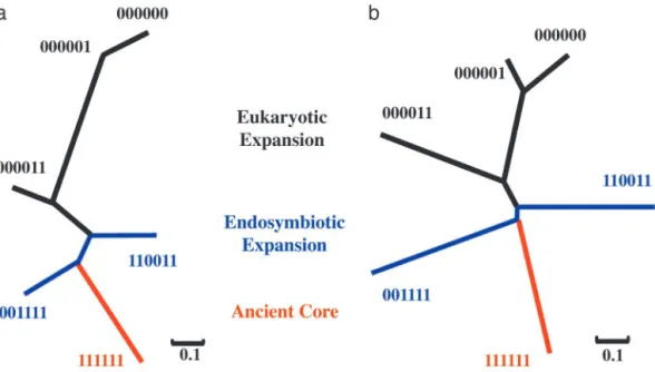
recon-structed the main growth path of the network from the inter-action patterns among the following six major isotemporal categories: b000000, b000001, b000011, b001111, b110011, and b111111. In our designed isotemporal categories, there are two groups of genomes for each domain of life (Eubacteria, Archaea, and Eukaryotes) (38). Categories b000011, b001111, b110011, and b111111 contain identical orthologous hits in both groups of genomes in each domain of life, and they are informative about the root of the universal tree of life (19, 38). Categories b000001

and b000000 may reveal the recent evolutionary history of the yeast. Furthermore, these six categories have large sample sizes. We converted the Z score of intercategory interaction ten-dency into distance (dz) through a logit-like transformation, dz⫽

1兾(1 ⫹ eZ_{), which transforms the Z scores into the range (0, 1).}

Positive Z scores correspond to small dz values because they

indicate that the observed intercategory interactions are above random expectations. Conversely, negative Z scores correspond to large dzvalues. From the dzdistance matrix, we inferred an NJ

tree (42) that describes the intercategory interaction tendencies of the major isotemporal categories (Fig. 3a). This tree is essentially the blueprint that accounts for the expansion of the protein interaction network, by means of the addition of groups of proteins to the network at various periods during evolution. The main assembling order of the major groups is represented by the path from the ancient proteins (b111111) to eukaryote-conserved proteins (b000011) and then to recent proteins (b000001 and b000000). Assuming that there existed an ancestral protein interaction network represented by the b111111 nodes, and assuming that network evolution can be described by node additions, the path from the ancient proteins to the recent ones in the NJ tree would thereby describe the major path of the network growth.

The positioning of b001111 (conserved between Archaea and Eukaryotes) and b110011 (conserved between Eubacteria and Eukaryotes) is consistent with the symbiotic hypothesis of the eukaryotic origin that argues for an archaeal host and a eubac-terial symbiont (43).

Likewise, through the transformation, d⬘z ⫽ 1兾(1⫹ e⫺Z), of

the Z scores of the average shortest paths, we inferred an NJ tree with the same branching pattern (Fig. 3b). Therefore, by using two independent measurements, we observed that network evolution mirrors the universal tree of life.

Isotemporal Clusters in the Network. By using a single-linkage

clustering method (44), we isolated the isotemporal clusters in the yeast protein interaction network by merging interacting proteins from the same isotemporal category into one node (see Fig. 6, which is published as supporting information on the PNAS

Fig. 2. Interaction patterns. (a) Z scores for all possible interactions of the isotemporal categories in the protein interaction network. For categories i and j, Z(i, j)⫽

[F(i,j)obs⫺ F(i,j)mean]兾␴(i, j), where F(i,j)obsis the observed number of interactions, F(i,j)meanand␴(i, j)are the average number of interactions and the SD, respectively, in 10,000

MS02 null models (37). A cutoff value of 10 is chosen in this presentation. The data matrix is in Table 2, which is published as supporting information on the PNAS web site. (b) Z scores for the average shortest paths of the isotemporal categories in the largest component of the analyzed protein interaction network. For categories i and j, Z(i, j)⫽ [d(i,j)obs⫺ d(i,j)mean]兾␴(i, j)where d(i,j)obsis the observed average shortest path, d(i,j)meanand␴(i, j)are the averaged average shortest path and the SD, respectively, in 500 isomorphic MS02 null models. A cutoff value of 5 is chosen in this presentation. The data matrix is in Table 3, which is published as supporting information on the PNAS web site.