License or Entry in Duopoly with Quality
Improving Innovation: Alternative Definitions of
License Fee
Masahiko Hattori
Faculty of Economics, Doshisha University, Japan
Yasuhito Tanaka
Faculty of Economics, Doshisha University, Japan
We examine the profitability of licensing a technology for producing a higher quality good or the same good at lower cost with or without entry into the market by an outside innovating firm under vertical product differentiation with ex-ante quality choice in duopoly. According to the definition of license fee by Kamien and Tauman (1986), the license with entry strategy is more profitable than the license without entry strategy for the innovating firm. However, the definition by Kamien and Tauman (1986) is inappropriate when the innovating firm has an option to enter the market, and if we adopt an alternative and more appropriate definition, the license without entry strategy is more profitable. We also show that the social welfare when the license fee is determined according to the alternative definition is lower than that when the license fee is determined according to the definition by Kamien and Tauman (1986) because in the latter case, the innovating firm enters the market; on the other hand, in the former case, it does not enter.
Keywords:ex-ante quality choice, technology development, license, market entry
JEL classification:D43, L13
*Correspondence to: Faculty of Economics, Doshisha University, Kamigyo-ku, Kyoto 602-8580, Japan. E-mail: [email protected].
1
□
Introduction
In this paper, we examine the profitability of licensing a technology for producing a higher quality good or the same good at lower cost with or without entry into the market by an outside innovating firm under vertical product differentiation with ex-ante quality choice in duopoly. According to the definition of license fee by Kamien and Tauman (1986), the license with entry strategy is more profitable than the license without entry strategy for the innovating firm. However, this definition is inappropriate from the game theoretic view point when the innovating firm has an option to enter the market, and if we adopt an alternative and more appropriate definition, the license without entry strategy is more profitable. We also show that when the license fee is determined according to the alternative definition, social welfare is lower than in the case when the license fee is determined according to the definition by Kamien and Tauman (1986). We show the following results in Propositions 1-6.
In the Cournot duopoly case, according to the definition of license fee by Kamien and Tauman (1986), the license with entry strategy is more profitable than the license without entry strategy, the former being the optimum strategy for the innovating firm; on the other hand, according to the alternative definition of license fee in the license without entry case, the license without entry strategy is more profitable than that with the entry strategy, and the former is the optimum strategy for the innovating firm.
In the Bertrand duopoly case, according to Kamien and Tauman’s (1986) definition, the license with entry strategy is more profitable than the license without entry strategy; however, the entry without license strategy is optimum for the innovating firm. On the other hand, according to the alternative definition of license fee, the license without entry strategy is more profitable than the license with entry strategy, the former being the optimum strategy for the innovating firm.
In both the Cournot and the Bertrand cases, the social welfare when the innovating firm chooses its strategy based on the alternative definition of license fee is smaller than that when it chooses its strategy based on the definition of license fee according to Kamien and Tauman (1986), because in the latter case, the innovating
firm enters the market, while in the former, it does not.
In the next section, we argue about the definition of license fee by Kamien and Tauman (1986) and our alternative definition. We also present a literature review and explain how this paper relates to previous studies. In Section 3, we present the model used in this paper. In Sections 4-7, we analyze behaviors of firms and social welfare in each of the cases, namely, before license and entry, entry without license, license with entry, and license without entry. In Section 8, we investigate the optimum strategy for the innovating firm, and in Section 9, we conclude the paper.
2
□
Literature Review
According to Proposition 4 in Kamien and Tauman (1986), in an oligopoly, when the number of firms is small (or very large), the strategy of entering the market and simultaneously licensing the cost-reducing technology to the incumbent firm (the license with entry strategy) is more profitable for the innovating firm than one where technology is licensed to the incumbent firm without entering the market (the license without entry strategy). However, their result depends on their definition of license fee. Interpreting their analysis in a duopoly model, they defined the license fee in the case of license without entry as the difference between the profit of the incumbent firm in that case and its monopoly profit before entry and license. However, if the license fee negotiation between the innovating firm and the incumbent firm breaks down, that is, the offered license fee is refused by the incumbent firm, the innovating firm can punish the incumbent firm by entering the market without a license. The innovating firm may use this threat if and only if it is credible. When the innovating firm neither enters nor sells a license, its profit is zero; however, when it enters the market without a license, its profit is positive. Therefore, such a threat is credible. Then, even if the innovating firm does not enter the market, the incumbent firm must pay the difference between its profit when it uses the new technology and its profit when the innovating firm enters without a license as a license fee.
In reality, the negotiation does not break down. In other words, the threat is determined such that the offered license fee is accepted by the incumbent firm within the limit.
We extend the analysis to a case of vertical product differentiation with ex-ante quality choice by firms using a model adapted from Nguyen (2014) and Nguyen et
al. (2014). Nguyen et al. (2014) analyzed a licensing problem in a duopoly with a
foreign innovating firm having a new technology to produce a higher quality good at no cost. However, in their model, the quality of the good produced by the new superior technology is fixed as 1, and a firm, which does not buy a license, chooses the quality of its good between 0 and 1. In this sense, the quality choice by firms in their model is not fully endogenous. In our model, both firms choose the quality of the goods between 0 and 1.
Various studies focus on technology adoption or R&D investment in duopoly or oligopoly. Most of them analyze the relation between the technology licensor and licensee. The difference of means of contracts, which comprise royalties, upfront fixed fees, combinations of these two, and auctions, are well discussed (Katz and Shapiro, 1985). Kamien and Tauman (2002) show that outside innovators prefer auctions, but industry incumbents prefer royalty. This topic is discussed by Kabiraj (2004) under the Stackelberg oligopoly; here, the licensor does not have production capacity. Wang and Yang (2004) consider the case when the licensor has production capacity.
Sen and Tauman (2007) compared the license system in detail, namely, when the licensor is an outsider and when it is an incumbent firm, using the combination of royalties and fixed fees. However, the existence of production capacity was externally given, and they did not analyze the choice of entry. Therefore, the optimal strategies of outside innovators, who can use the entry as a threat, require more discussion. Regarding the strategies of new entrants to the market, Duchene et al. (2015) focused on future entrants with old technology, and argued that while a low license fee can be used to deter the entry of potential entrants, the firm with new technology is incumbent, and its choice of entry is not analyzed. Also, Chen (2016) analyzed the model of the endogenous market structure determined by the potential entrant with old technology and showed that the licensor uses the fixed fee and zero royalty in both the incumbent and the outside innovator cases, which are exogenously given.
Below, we present a brief review of studies that analyzed related topics. A Cournot oligopoly with fixed fee under cost asymmetry was analyzed by La Manna
(1993). He showed that if technologies can be replicated perfectly, a lower cost firm always has the incentive to transfer its technology; hence, while a Cournot–Nash equilibrium cannot be fully asymmetric, there exists no non-cooperative Nash equilibrium in pure strategies. On the other hand, using cooperative game theory, Watanabe and Muto (2008) analyzed bargaining between a licensor with no production capacity and oligopolistic firms. Recent research focuses on market structure and technology improvement. Boone (2001) and Matsumura et al. (2013) found a non-monotonic relation between intensity of competition and innovation. Also, Pal (2010) showed that technology adoption may change the market outcome. The social welfare is larger in Bertrand competition than in Cournot competition. However, if we consider technology adoption, Cournot competition may result in higher social welfare than Bertrand competition under a differentiated goods market. Hattori and Tanaka (2014, 2015) studied the adoption of new technology in Cournot duopoly and Stackelberg duopoly. Rebolledo and Sandonís (2012) presented an analysis of the effectiveness of research and development (R&D) subsidies in an oligopolistic model in the cases of international competition and cooperation in R&D.
3
□
The Model
There are two firms, Firms A and B, in an industry. Firm A is an outside innovating firm, and Firm B is an incumbent firm. At present, only Firm B monopolistically produces a good of some quality. Firm A has a superior new technology. It can produce a higher quality good at the same cost or produce the same good at lower cost. Firm A has three options. The first option is to enter the market without a license for the new technology. The second option is to enter the market and simultaneously license its technology to Firm B. The third option is to license its technology to Firm B without entering the market. We consider a fixed license fee. Let qA be the quality of the good supplied by Firm A, and qB be the quality of Firm B’s good, where 0 <qA< 1 and 0 <qB< 1.
We suppose the following market structure. There is a continuum of consumers with the same income, denoted by y , but different values of the taste parameter. The taste parameter of consumers is denoted by . Each consumer buys at most
one unit of the good. If a consumer with parameter buys one unit of a good of quality q at price p , his utility is equal to y p q. If a consumer does not buy the good, his utility is equal to his income y . The parameter is distributed according to a smooth distribution function =F( ) in the interval 0 <1. denotes the probability that the taste parameter is smaller than or equal to . The size of the market, that is, the volume of consumers, is normalized as one. Let us suppose that F( ) has a uniform distribution, then = .
Let pA and pB be the prices of the goods of Firms A and B respectively, and let xA and xB be the outputs of Firms A and B respectively. We consider a two-stage Cournot or Bertrand game with ex-ante quality choice. In the first stage, the firms (one firm or both firms) choose the quality of their goods. In the second stage, they determine their outputs or the prices of their goods. The constant marginal costs are 2
(1/ 2)qA for Firm A and 2 B
q for Firm B. If Firm B buys a license to use the new technology from Firm A, its marginal cost is also 2
(1/ 2)qB.
There are four cases. Let us analyze each case in the following sections.
4
□
Before License and Entry
We use this case as the benchmark case for the determination of the license fee in the license without entry case according to the definition by Kamien and Tauman (1986). If Firm A does not license its technology for producing a higher quality good to Firm B and does not enter the market, Firm B is a monopolist with its old technology. Let
B be the value of for which the corresponding consumer is indifferent between buying nothing and buying the good of quality qB. Then,=
B B B
q
p , and so, B= pB/qB. Since the volume of consumers is normalized as one, the direct demand function of the good of quality qB is:= 1 = 1 B B B B p x q . B
x denotes the supply of the good of quality qB in the market. We have
0 <xB< 1. The inverse demand function is obtained as follows:
= = (1 )
B B B B B
Since 0 < 1xB< 1, we have 0 <pB<qB. The profit of Firm B is:
2 2
= = (1 )
B p qB B q xB B qB x xB B q xB B
.The condition for profit maximization of Firm B with respect to its output is:
2
2 = 0
B B B B
q q x q .
The equilibrium values of the output and profit respectively are obtained as follows.
1 = 2 B B q x , and
2 (1 ) = 4 B B B q q .
Firm B chooses qB to maximize
B. The condition for maximization of
B is: 21 4 qB3qB = (1qB)(1 3 ) = 0 qB .
Thus, it chooses the quality:
1
= 0.3333
3
B
q . (1)
Its profit is:
1
= 0.0370
27
B
. (2)
Denote
B in this case by m B
.5
□
Entry without License Case
Suppose that Firm A enters the market without the license to Firm B. Firm A produces a good of quality qA, and Firm B produces a good of quality qB. We assume qA>qB. This case is also a benchmark case, and we use it to determine the
license fee in the license without entry case with regard to the alternative definition of license fee. Moreover, the innovating firm may choose this strategy under
Bertrand duopoly. We consider two cases, Cournot and Bertrand.
5.1
□
Cournot Dopoly
Let
B be the value of for which the corresponding consumer is indifferent between buying nothing and buying Firm B’s good. Then, B =pB/qB. Let
A be the value of for which the corresponding consumer is indifferent between buying Firm A’s good and buying Firm B’s good. Then,
AqBpB=
AqApA, and so, A(pApB) / (qAqB). We assume 0 <
B<
A< 1. The direct demand function for the good of Firm A is:= 1 = 1 A B A A A B p p x q q ,
and the direct demand function for the good of Firm B is:
= = A B B B A B A B B p p p x q q q .
We have 0 <xB < 1 and 0 <xA< 1. The inverse demand functions are:
= (
)
= (
)(1
)
(1
)
A A B A B B A B A B A B
p
q
q
q
q
q
x
q
x
x
for Firm A’s good, and
= = (1 )
B B B B A B
p q
q x xfor Firm B’s good. Since 1xAxB< 1xA< 1, we have pB<qB and pA <qA.
The profits of Firms A and B are written as:
2 2 1 1 = = [( )(1 ) (1 )] 2 2 A p xA A q xA A qA qB xA qB xA xB xA q xA A , and 2 2 = = (1 ) B p xB B q xB B qB xA x xB B q xB B
.The first order conditions for profit maximization of Firms A and B with respect to their outputs are:
2 2 1 = ( )(1 ) (1 ) 2 1 = 0, 2 A A A A A B A B A B A A A p q x q q q x q x x q x q and
2 2 = (1 ) = 0 B B B B B A B B B B p q x q q x x q x q .
Solving them, we obtain the equilibrium outputs of Firms A and B as follows.
2 2 2 = 4 A B A B A A B q q q q x q q , and
(2 4 ) = 2(4 ) A A B B A B q q q x q q .
Then, the equilibrium profits of Firms A and B are:
2 2 2 2 (2 ) = (4 ) A A B A B A A B q q q q q q q
, and 2 2 2 (2 4 ) = 4(4 ) A B A B B A B q q q q q q
.The firms choose the quality of their goods to maximize their profits. The conditions for profit maximization with respect to the quality are:
3 2 2 2 3 2
4 5 2 12 8 = 0
B A B B A B A B A A
q q q q q q q q q q
for Firm A and
2 2
4qB47q qA B2qB4qA8qA= 0
for Firm B. Since these equations are complex, we solve them numerically. Then, the values of the equilibrium quality of the goods of Firm A and Firm B are:
0.6882, 0.2523
A B
The equilibrium profits of the firms are:
0.0561,
0.0135
A B
. (4)Denote
A and
B in this case by e A
and e B
.When the innovating firm enters the market, consumers’ surplus, CS , is calculated as follows. 1 1 2 2 2 2 2 2 2 = ( ) ( ) 1 1 = [( ) ] 2 2 1 = (1 ) [( ) ](1 ) 2 1 ( ) ( ) 2 1 1 = (1 ) ( )[2(1 ) ( )] 2 2 1 = 2 A A A B B A B A A A B A B B B B B A B A A A B A B B A B A B B B A B A A B A B A A B A A CS q p d q p d q q q q q q q q q q q q q q q x
2 1 . 2 B A B B B q x x q x From the equilibrium values of the outputs and qualities in this case, we get:
0.0515 e CS with = 0.2856, = 0.2311 A B x x .
The total output is 0.5167. The social welfare in this case, e
W , is the sum of the
consumers’ surplus and the profits of the firms. It is:
= 0.0515 0.0561 0.0135 = 0.1211
e e e e
A B
W CS . (5)
5.2
□
Bertrand Duopoly
2 2 1 1 = = 1 2 2 A B A A A A A A A B p p p q x p q q q
, and2 2 = ( ) = A B B ( ) B B B B B B A B B p p p p q x p q q q q
.The first order conditions for profit maximization with respect to the prices for Firms A and B are:
2 2 2 2 4 = 0 2( ) B A A B A B A q q q p p q q , and
2 2 = 0 ( ) A B A B B A B B A q q p q p q q q q .
The equilibrium prices of the goods of Firms A and B are:
2 2 ( 2 2 ) = 4 A B B A A A A B q q q q q p q q , and 2 (4 2 2 ) = 2(4 ) B A B B A A B A B q q q q q q p q q .
The equilibrium outputs of Firms A and B are:
2 2 (2 4 2 4 ) = 2( 4 )( ) A B A B B A A A B A B A q q q q q q q x q q q q , and
2 2 (2 4 2 2 ) = 2( 4 )( ) A B A B B A A B B A B A q q q q q q q x q q q q .
2 2 2 2 2 (2 4 2 4 ) = 4( 4 ) ( ) A B A B B A A A B A A B q q q q q q q q q q q
, and 2 2 2 2 (2 4 2 2 ) = 4( 4 ) ( ) A B B A B B A A B B A A B q q q q q q q q q q q q
.The firms choose the qualities of their goods to maximize their profits. The conditions for profit maximization with respect to the quality are:
4 3 3 2 2 2 3 2 4 3 4 2 8 31 20 46 28 24 16 = 0 B A B B A B A B A B A B A A q q q q q q q q q q q q q q
for Firm A and
4 3 2 2 2 3 2 4 3 4 38 74 14 47 22 4 8 = 0 B A B A B A B A B A B A A q q q q q q q q q q q q q
for Firm B. We solve them numerically. Then, the values of the equilibrium quality of the goods of Firm A and B are:
0.7084, 0.1979
A B
q q . (6)
The equilibrium profits of the firms are:
0.0559, 0.0107
A B
. (7)
Denote
A and
B in this case by e A
and e B
. The consumers’ surplus in this case is:= 0.0641 e CS , with
= 0.3309, = 0.2739 A B x x .
The total output is 0.6048 . The social welfare is:
0.0641 0.0559 0.0107 = 0.1307
e
6
□
License with Entry Case
Suppose that Firm A enters the market and simultaneously licenses its technology to Firm B. We assume qA >qB. Alternatively, we can assume qB >qA.
1
However, in that case, the results for Firms A and B are simply interchanged, and the total profit of Firm A, including the license fee, when qB >qA is equal to its total profit when
>
A B
q q . Also, the social welfare in both cases is equal. We consider two cases, Cournot and Bertrand.
6.1
□
Cournot Duopoly
Let
B and
A have the same meanings as those in the previous case. Then,= /
B pB qB
and A(pApB) / (qAqB). The direct demand functions for the goods are:
= 1 A B, = A B B A B A B A B B p p p p p x x q q q q q .
The inverse demand functions are:
= ( )(1 ) (1 ), = (1 )
A A B A B A B B B A B
p q q x q x x p q x x .
The profits of Firms A and B are written as:
2 1 = [( )(1 ) (1 )] 2 A qA qB xA qB xA xB xA q xA A , and 2 1 = (1 ) 2 B qB xA x xB B q xB B L .
L is a fixed license fee. The first order conditions for profit maximization of Firms
A and B with respect to the outputs are:
1 At equilibrium, no firm chooses the same quality as that of the rival firm’s good; thus,
B q A q .
2 1 ( )(1 ) (1 ) = 0 2 A B A B A B A A A q q x q x x q x q , and 2 1 (1 ) = 0 2 B A B B B B q x x q x q .
The equilibrium outputs of Firms A and B are:
2 2 2 2 4 = (2(4 ) B B A A A A B q q q q x q q , and (2 2 ) = 2(4 ) A A B B A B q q q x q q .
The equilibrium profits of Firms A and B are obtained as follows.
2 2 2 2 ( 2 2 4 ) = 4(4 ) A B B A A A A B q q q q q q q
, and2 2 2 (2 2) = 4( 4 ) A B B A B B A q q q q L q q
.The firms choose the quality of their goods to maximize their profits. The conditions for profit maximization with respect to the quality are:
3 2 2 2 3 2
4 2 10 4 24 16 = 0
B A B B A B A B A A
q q q q q q q q q q
for Firm A and
2 2
2qB23q qA B2qB4qA8qA= 0
for Firm B. We also solve them numerically. Then, the values of the equilibrium quality of the goods of Firms A and B are:
0.7381, 0.5856
A B
The equilibrium profits of the firms are:
0.0353, 0.0350
A B L
. (10)
Denote
A,
B, and L in this case by el A
, elB
, and elL respectively. The total profit of Firm A is el el
A L
.The consumers’ surplus in this case is:
= 0.0664 el CS , with
= 0.2186, = 0.2443 A B x x .
The total output is 0.4629 . The social welfare, el W , is: = 0.0664 0.0353 0.0350 = 0.1367 el el el el A B W CS
. (11)6.2 Bertrand Duopoly
The profits of Firms A and B are written as follows.
2 1 = 1 2 A B A A A A B p p p q q q
, and 2 1 = 2 A B B B B B A B B p p p p q L q q q
.The first order conditions for profit maximization with respect to the prices for Firms A and B respectively are:
2 2 2 2 4 0 2( ) B A A B A B A q q q p p q q , and 2 2 4 0 2 ( ) A B A B B A B B A q q p q p q q q q .
The equilibrium prices of the goods of Firms A and B are: 2 2 ( 4 2 4 ) = 2(4 ) A B B A A A A B q q q q q p q q , and
2 (2 2 2 ) = 2(4 ) B A B B A A B A B q q q q q q p q q .
The equilibrium outputs of Firms A and B are:
(4 2 ) = 2(4 ) A B A A A B q q q x q q , and
(2 ) = 2(4 ) A B A B A B q q q x q q .
The equilibrium profits of Firms A and B are:
2 2 2 ( )( 2 4) = 4( 4 ) A A B B A A B A q q q q q q q
, and2 2 ( 2) ( ) = 4( 4 ) A B B A A B B B A q q q q q q L q q
.L is a fixed license fee. The firms choose the quality of their goods to maximize
their profits. The conditions for profit maximization with respect to the qualities are:
3 2 2 2 3 2
2qB5q qA B8qB22q qA B12q qA B24qA16qA= 0
for Firm A and
3 2 2 3 2
2qB17q qA B19q qA B14q qA B4qA8qA= 0
for Firm B. We solve them numerically. Then, the values of the equilibrium quality of the goods of Firms A and B are:
0.8195, 0.3987
A B
q q . (12)
The equilibrium profits of the firms are:
0.0328, 0.0243
A B L
. (13)
Denote
A,
B, and L in this case by el A
, elB
, and elL respectively. The total
profit of Firm A is el el A L
.The consumers’ surplus in this case is: = 0.094 el CS with = 0.2792, = 0.3445 A B x x .
The total output is 0.6237 . The social welfare is:
0.094 0.0328 0.0243 = 0.1511
el
W . (14)
7 License without Entry Case
Suppose that Firm A licenses its technology to Firm B, but does not enter the market. Then, Firm B produces its good at a lower cost, and it is a monopolist. The direct demand function for its good is:
= 1 B B B p x q .
The inverse demand function is:
= (1 )
B B B
p q x .
The profit and condition for profit maximization of Firm B respectively are:
2 1 = (1 ) 2 B qB x xB B q xB B L , and
2 1 (1 2 ) = 0 2 B B B q x q .
L is a fixed license fee. The equilibrium output and profit respectively are:
2 2 (2 ) = , = 4 16 B B B B B q q q x
.Then, the condition for profit maximization with respect to the quality is:
2
4 4 qB3qB = (2qB)(2 3 qB) = 0. Firm B chooses the quality:
2
= 0.6667 3
B
q . (15)
Its profit is:
2
= 0.0741 27
B L L
. (16)Denote
B and L in this case by l B
and lL respectively.
When the innovating firm does not enter, consumers’ surplus, CS , is calculated as follows. 1 1 1 2 1 2 1 2 = ( ) = = (1 ) = 2 2 2 B B B B B B B B B B B CS q p d q q q q x
.From the equilibrium values of the output and quality in this case, we get:
1 = 0.0370 27 l CS , with
1 = 0.3333 3 B x .
The social welfare, W , in this case is: l
= 0.0370 0.0741 = 0.1111
l l l
B
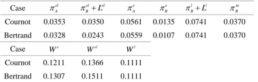
We summarize the results in the following table.
Table 1. Summary of the Results in Each Strategy
Case
elA el el B L
e A
e B
l l B L
m B
Cournot 0.0353 0.0350 0.0561 0.0135 0.0741 0.0370 Bertrand 0.0328 0.0243 0.0559 0.0107 0.0741 0.0370 Case e W el W l W Cournot 0.1211 0.1366 0.1111 Bertrand 0.1307 0.1511 0.11118
□
License Fees and Optimum Strategies for the
Innovating Firm
8.1
□
Cournot Duopoly Case
8.1.1□Definition of License Fee in Kamien and Tauman (1986)
Translating their analysis into a duopoly model, Kamien and Tauman (1986) defined the license fee in the license with entry case as the difference between the profit of Firm B in that case and its profit when Firm A enters the market without a license to Firm B as follows.2
= ( ) = 0.0350 0.0135 = 0.0215
el el el e
B B
L L .
The total profit of Firm A in the license with entry case is the sum of the license fee and its profit as a firm in the duopoly. It is equal to:
= 0.0353 0.0215 = 0.0568
el el A L
.
On the other hand, they defined the license fee in the license without entry case as the difference between the profit of Firm B in that case and its profit before license
2 This equation means
= el e B B .
and entry as follows.3 = ( ) = 0.0741 0.0370 = 0.0371 l l l m B B L L . Comparing l L and el el A L
, ( ) = 0.0371 0.0568 = 0.0197 < 0 l el el A L L , and we have: = 0.0568 0.0561 = 0.0007 > 0 el el e A L A .Thus, the license with entry strategy is optimum. We have shown the following result.
Proposition 1 In the Cournot duopoly case, according to the definition of license fee by Kamien and Tauman (1986), the license with entry strategy is more profitable than the license without entry strategy, and the former is the optimum strategy for the innovating firm.
When the innovating firm chooses its optimum strategy, the social welfare is 0.1366.
8.1.2□Alternative Definition of License Fee
If the negotiation about the license fee between Firms A and B breaks down, Firm A can enter the market without license to Firm B. As stated in the Introduction, the negotiation does not break down in reality. In other words, the threat is determined such that the offered license fee is accepted by the incumbent firm within the limit.
Comparing e B
and m B
yields: = 0.0135 0.0370 = 0.0235 < 0 e m B B .Thus, entry without license entails more severe punishment than no license without entry.
If Firm A does not enter the market nor license its technology, its profit is zero.
3 This equation means
= l m B B .
However, if it enters the market, its profit ( e A
) is positive. Therefore, such a threat is credible, and hence, Firm B must pay the difference between its profit in the license without entry case and its profit in the entry without license case as a license fee. Then, we obtain:= ( ) = 0.0741 0.0135 = 0.0606 l l l e B B L L . el el A L
is common to the previous case. Comparing lL in this case and el el A L
yields: ( ) = 0.0606 0.0568 = 0.0038 > 0 l el el A L L , and we have: = 0.0606 0.0561 = 0.0044 > 0 l e A L .Thus, in this case, the license without entry strategy is optimum. We have shown the following.
Proposition 2 In the Cournot duopoly case, according to the alternative definition of license fee in the license without entry case, the license without entry strategy is more profitable than the license with entry strategy, and it is the optimum strategy for the innovating firm.
When the innovating firm chooses its optimum strategy, the social welfare is 0.1111, which is smaller than 0.1366 . Therefore, we devise Proposition 3.
Proposition 3 In the Cournot duopoly, the social welfare when the innovating firm chooses its strategy based on the alternative definition of license fee is smaller than that when it chooses its strategy based on the definition of license fee according to Kamien and Tauman (1986).
8.2
□
Bertrand Duopoly Case
8.2.1□Definition of License Fee in Kamien and Tauman (1986)
= ( ) = 0.0243 0.0107 = 0.0136
el el el e
B B
L L .
The total profit of Firm A in the license with entry case is:
= 0.0328 0.0136 = 0.0464
el el A L
.
l
L is common to the Cournot duopoly case. Comparing l
L and el el A L
, ( ) = 0.0371 0.0464 = 0.0093 < 0 l el el A L L , and we have = 0.0464 0.0559 < 0.0095 < 0 el el e A L A .Thus, in this case, entry without license strategy is optimum. We have shown the following result.
Proposition 4 In the Bertrand duopoly case, according to the definition of license fee by Kamien and Tauman (1986), the license with entry strategy is more profitable than the license without entry strategy; however, the entry without license strategy is optimum for the innovating firm.
If the innovating firm chooses its strategy based on the definition of license fee by Kamien and Tauman (1986), it enters the market in both the Cournot and the Bertrand duopoly cases. When the innovating firm chooses its optimum strategy under Bertrand duopoly, the social welfare is 0.1307.
8.2.2□Alternative Definition of License Fee
Similar to the Cournot duopoly, if the negotiation about the license fee between Firms A and B breaks down, Firm A can enter the market without license to Firm B.
Comparing e B
and m B
yields: = 0.0107 0.0370 = 0.0263 < 0 e m B B .Thus, in this case also, entry without license entails a more severe punishment than no license without entry.
However, if it enters the market, its profit ( e A
) is positive. Therefore, such a threat is credible, and hence, Firm B must pay the difference between its profit in the license without entry case and its profit in the entry without license case as a license fee. Then, we obtain:= ( ) = 0.0741 0.0107 = 0.0634 l l l e B B L L . el el A L
is common to the previous case. Comparing lL in this case and el el A L
yields: ( ) = 0.0634 0.0464 = 0.0170 > 0 l el el A L L , and we have: = 0.0634 0.0559 = 0.0075 > 0 l e A L .Thus, in this case, the license without entry strategy is optimum. We have shown the following.
Proposition 5 In the Bertrand duopoly case, according to the alternative definition of license fee in the license without entry case, the license without entry strategy is more profitable than the license with entry strategy, and it is the optimum strategy for the innovating firm.
If the innovating firm chooses its strategy based on the alternative definition of license fee, it does not enter the market in both the Cournot and the Bertrand duopoly cases. When the innovating firm chooses its optimum strategy, the social welfare is 0.1111, which is smaller than 0.1307.
Proposition 6 In the Bertrand duopoly, the social welfare when the innovating firm chooses its strategy based on the alternative definition of license fee is smaller than that when it chooses its strategy based on the definition according to Kamien and Tauman (1986).
Of course, the differences between Propositions 1 and 2 and between Propositions 4 and 5 are due to the difference between the two definitions of license fees in the case of license without entry. In the definition by Kamien and Tauman (1986), the license fee in that case is equal to the profit of the incumbent firm and its
profit before license and entry. However, by the alternative definition, it is equal to the profit of the incumbent firm and its profit when the innovating firm enters the market without license to the incumbent firm. As we have argued above, in the case of license without entry, the threat by the innovating firm to enter the market during the negotiation with the incumbent firm is credible. Therefore, the license fee in that case under the alternative definition is larger than that under the definition by Kamien and Tauman (1986).
When the innovating firm chooses its strategy based on the alternative definition, it does not enter the market in both the Cournot and the Bertrand cases; then, the incumbent firm is a monopolist. On the other hand, when the innovating firm chooses its strategy based on the definition by Kamien and Tauman (1986), it enters the market with or without license; then, the market becomes duopolistic. The difference in the social welfare between Propositions 3 and 6 is due to this fact.
9
□
Concluding Remarks
We analyzed the choice of an outside innovating firm in a duopoly having ex-ante quality choice to license its technology for producing a higher quality good or the same good at lower cost to an incumbent firm with or without entering the market. We have shown that the optimum choice of the innovating firm depends on the definition of license fee. Under the definition by Kamien and Tauman (1986), the license with entry (or the entry without license) strategy is optimum; however, under the alternative definition of license fee, only the license without entry strategy is optimum for the innovating firm.
In future research, we shall study the problem in oligopoly and also analyze how government public policy may promote or prevent license or entry by the innovating firm.
Acknowledgment
We thank the referees for carefully reading our manuscript and giving useful comments. This work was supported by JSPS KAKENHI Grant Number 15K03481.
References
Boone, J., (2001), “Intensity of Competition and the Incentive to Innovate,”
International Journal of Industrial Organization, 19, 705-726.
Chen, C.-S., (2016), “Endogenous Market Structure and Technology Licensing,”
Japanese Economic Review, forthcoming.
Duchene, A., D. Sen, and K. Serfes, (2015), “Patent Licensing and Entry Deterrence: The Role of Low Royalties,” Economica, 82, 1324-1348.
Hattori, M. and Y. Tanaka, (2014), “Incentive for Adoption of New Technology in Duopoly under Absolute and Relative Profit Maximization,” Economics
Bulletin, 34, 2051-2059.
Hattori, M. and Y. Tanaka, (2015), “Subsidizing New Technology Adoption in a Stackelberg Duopoly: Cases of Substitutes and Complements,” Italian
Economic Journal, 2, 197-215.
Kabiraj, T., (2004), “Patent Licensing in a Leadership Structure,” The Manchester
School, 72, 188-205.
Kamien, T. and Y. Tauman, (1986), “Fees versus Royalties and the Private Value of a Patent,” Quarterly Journal of Economics, 101, 471-492.
Kamien, T. and Y. Tauman, (2002), “Patent Licensing: The Inside Story,” The
Manchester School, 70, 7-15.
Katz, M. and C. Shapiro, (1985), “On the Licensing of Innovations,” Rand Journal
of Economics, 16, 504-520.
La Manna, M., (1993), “Asymmetric Oligopoly and Technology Transfers,”
Economic Journal, 103, 436-443.
Matsumura, T., N. Matsushima, and S. Cato, (2013), “Competitiveness and R&D Competition Revisited,” Economic Modelling, 31, 541-547.
Nguyen, X., (2014), “Licensing under Vertical Product Differentiation: Price vs. Quantity Competition,” Economic Modelling, 36, 600-606.
Nguyen, X., P. Sgro, and M. Nabin, (2014), “Monopolistic Third-degree Price Discrimination under Vertical Product Differentiation,” Economics Letters, 125, 153-155.
Pal, R., (2010), “Technology Adoption in a Differentiated Duopoly: Cournot versus Bertrand,” Research in Economics, 64, 128-136.
Rebolledo, M. and J. Sandonís, (2012), “The Effectiveness of R&D Subsidies,”
Economics of Innovation and New Technology, 21, 815-825.
Sen, D. and Y. Tauman, (2007), “General Licensing Schemes for a Cost-reducing Innovation,” Games and Economic Behavior, 59, 163-186.
Wang, X. H. and B. Z. Yang, (2004), “On Technology Licensing in a Stackelberg Duopoly,” Australian Economic Papers, 43, 448-458.
Watanabe, N. and S. Muto, (2008), “Stable Profit Sharing in a Patent Licensing Game: General Bargaining Outcomes,” International Journal of Game Theory, 37, 505-523.