長程演進網路下載系統基於部分頻率複用之協同式干擾避免機制

(1)

長程演進網路下載系統基於部分頻率複用之協同式干擾避免機制

Fraction Frequency Reuse-Based Inter-cell Interference Coordination

Mechanism for LTE Downlink Transmission

研究生：廖政博 Student：Zheng-Bo Liao

指導教授：趙禧綠 Advisor：His-Lu Chao

國立交通大學

網路工程學系

碩士論文

A Thesis

Submitted to Department of Network Engineering College of Computer Science

National Chiao Tung University in partial Fulfillment of the Requirements

for the Degree of Master

in

Computer Science July 2011

Hsinchu, Taiwan, Republic of China

(2)

i

摘要

近年來，無線通訊的使用人數持續上升，尤其對於多媒體傳輸的需求

更是大幅提升，為了達到這種需求，4G 行動通訊的發展正持續地在進行中，

其中 3GPP 提出的 Long Term Evolution (LTE) 便是其中一項技術。LTE 屬

於蜂巢式網路，這種系統架構下有個主要問題是基地台間的干擾問題，若

無法妥善的處理干擾問題，便無法達到高傳輸速率以及高覆蓋率的要求。

在傳統的靜態干擾避免機制下，會因為使用者分布的不同，而造成系

統資源的浪費，在本篇論文中，我們提出了一個基於部分頻率複用的動態

協同式干擾避免機制。透過此機制我們可以根據使用者分布的情形，動態

的調整高功率頻段和低功率頻段的範圍，用此方法來調整系統資源便不會

有資源浪費的問題

(3)

ii

Abstract

In recent year, people who need radio network are increasing, especially

for the multimedia communication. To reach such demand, 4G cellular

wireless network is working on. Long Term Evolution (LTE) is one of the 4G

standards proposed by 3GPP. LTE is a cellular network system; this kind of

system suffers from interference problem between cells. If we do not handle

interference well, we cannot reach the goal of high transmission rate and high

cell coverage.

In traditional static interference avoidance scheme, different user

distribution will cause wasting of resource. In this thesis we propose a

fractional frequency based dynamic interference coordination scheme. By the

scheme we can dynamic adjust the high power frequency band and normal

power frequency band according to user distribution. Adjusting frequency

band through this scheme can efficiently eliminate the resource wasting

problem.

(4)

iii

致謝

感謝這兩年來陪我一起走過的同學們，有問題時總是能互相幫忙與討

論，還有博班學姐在計畫上的幫忙，並且適時地提供些論文上面的靈感，

也很感謝學弟們時常揪團打牌和唱歌，讓我在寫論文時有管道可以抒發壓

力，最後要感謝爹娘對我放牛吃草式的教育方式，讓我念書起來沒有來自

於家庭的壓力，以及姊姊在我快餓死時的金援，不然不會有今天這篇論文

的，感謝大家！

(5)

iv

List of Figures

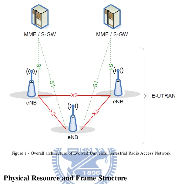
Figure 1 - Overall architecture of Evolved Universal Terrestrial Radio Access

Network... ...3

Figure 2 - The concept of Resource Block in LTE system...4

Figure 3 - The frame structure of FDD LTE system...4

Figure 4 - The frequency and power planning of reuse-1 and reuse-3...8

Figure 5 - Concept of Soft Frequency Reuse scheme...10

Figure 6 - Concept of Fractional Frequency Reuse scheme...11

Figure 7 - Concept of Enhanced Fractional Frequency Reuse scheme...12

Figure 8 - Concept of Incremental Frequency Reuse...14

Figure 9 - Example of user distribution problem...15

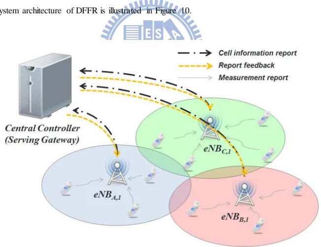
Figure 10 - System architecture of Dynamic Fractional Frequency

Reuse...17

Figure 11 - The system frequency-power configuration after frequency and

power allocation part of DFFR...23

Figure 12 - Pseudo code of frequency and power allocation at eNB...24

Figure 13 - Pseudo code of frequency and power allocation at central

controller...25

Figure 14 - Simulation system layout with 19 hexagonal cells...27

Figure 15 - Comparison of outage network probability between DFFR and

EFFR with different proportion in case of CEU:CCE = 8:2 UE

distritubtion...32

Figure 16 - Comparison of resource utilization efficiency between DFFR and

EFFR with different proportion in case of CEU:CCE = 8:2 UE

distribution...32

(7)

vi

Figure 17 - Comparison of CEU average throughput between DFFR and

EFFR with different proportion in case of CEU:CCU=8:2 UE

distribution...33

Figure 18 - Comparison of outage network proportion between DFFR and

EFFR with different proportion in case of CEU:CCU=5:5 UE

distribution...34

Figure 19 - Comparison of resource utilization efficiency between DFFR and

EFFR with different proportion in case of CEU:CCU=5:5 UE

(8)

vii

List of Tables

Table 1 - The SINR to data rate per RB mapping table...29

Table 2 - Simulation parameter list...30

(9)

8

Chapter 1 Introduction

As the growing up of mobile device users and the demand of wireless multimedia services, the higher speed wireless system is expected to be developed. There are many standardization bodies and forums work for this issue, for example, Third Generation Partnership Project Long Term Evolution (3GPP-LTE) [1], Wireless World Initiative New Radio (WINNER) [2] and Worldwide Interoperability for Microwave Access (WiMAX) [3]. All of these standardization bodies and forums focus at high peak data rate, low latency, improved system capacity and coverage and flexible bandwidth operation.

In 3GPP-LTE, the peak rate requirement for downlink and uplink are set at 100Mbps and 50Mbps respectively. As the data rate increases, the latency needs to be reduced to show the practical improvement. Thus the latency requirement for LTE radio round trip time is set to be below 10ms and access delay below 300ms [4]. For the flexible bandwidth operation requirement, LTE support flexible bandwidth range from 1.4 MHz to 20 MHz [4]. The multiple access scheme in LTE adopts Orthogonal Frequency Division Multiple Access (OFDMA) for downlink and Single Carrier Frequency Division Multiple Access (SC-FDMA) for uplink. The primary advantage of OFDM based system is its resistance to the intra-cell interference. Intra-cell interference from user equipment (UE) can be ignored because of the orthogonality of subcarriers. But the neighboring cells may occupy the same subcarriers for their serving UE at the same time, it will cause significant inter-cell interference (ICI) or so-called co-channel interference (CCI), especially for users located at cell edge.

The performance of today’s cellular network is limited by interference problem more than by any other single effect [5]. Interference between cells will scale down the cell coverage and reduce the UE’s data rate. So interference mitigation is one of the key issues currently under investigation in different standardization bodies and forums. Interference

(10)

9

mitigation techniques can be categorized into three main classes based on approaches adopted:

interference randomization, interference cancellation and interference coordination [6]. The

basic principle of these three approaches will be discussed in chapter 2.

1.1 E-UTRAN Architecture

3GPP proposes Evolved Universal Terrestrial Radio Access Network (E-UTRAN) as the air interface of LTE. The overall architecture of E-UTRAN is illustrated in Figure 1 [7]. In E-UTRAN, the macro base station is denoted as eNB (Evolved NodeB). The eNBs are interconnected with each other through X2 interface. The eNBs also connect to EPC (Evolved Packet Core) through S1 interface. For specifically description, EPC consist of MME (Mobility Management Entity) and S-GW (Serving Gateway). Main functions of MME in charging of are [4]

 Authentication and security.  Mobility management.

 Managing subscription profile and service connectivity. and S-GW has the following main functions [4]

 IP service mapping.

 User Plane Tunnels for uplink and downlink data delivery.  Downlink data forwarding for handover.

Through Figure 1 we can see that each eNB must connect to at least one MME/S-GW which means that an MME/S-GW is in charge of several eNBs. The proposed method in this thesis needs a central controller of eNBs which plays an important role in the algorithm. We can take MME/S-GW as central controller of a set of eNBs.

(11)

10

Figure 1 - Overall architecture of Evolved Universal Terrestrial Radio Access Network

1.2 Physical Resource and Frame Structure

Before talking about the resource allocation scheme, we need some background of LTE resource structure. The physical resource structure of LTE system for downlink and uplink is illustrated in Figure 2. The smallest resource unit in frequency domain is subcarrier which spacing is 15 kHz regardless of the total transmission bandwidth. The smallest time unit is so-called symbol which duration is 66.7 μs [4]. To put a subcarrier and a symbol together as a grid we call it resource element. But the minimum scheduling size is not resource element;

physical resource block (PRB or RB) is the basic scheduling unit both in uplink and downlink.

Physical resource block can be seen as a time- frequency grid which consists of 12 consecutive subcarriers in frequency domain. It means that the minimum bandwidth can be allocated is 180 kHz.

(12)

11

Figure 2 - The concept of Resource Block in LTE system

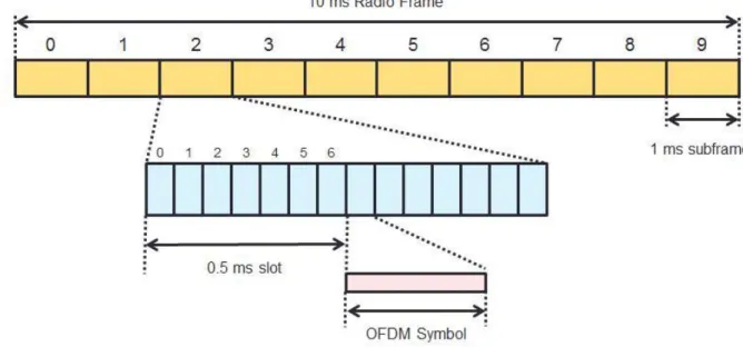
There are two frame structure types that support by LTE system. One type is used in FDD system and another type is used in TDD system. Here we focus on FDD system. The frame structure of FDD LTE system is illustrated in Figure 3. One radio frame has 10 ms duration which consists of 10 subframes with 1 ms duration. One subframe is combined with two 0.5 ms time slots which are composed of 14 OFDM symbols.

(13)

12

Combine the knowledge of physical resource structure and frame structure mentioned above. We know that in time domain physical resource block refers to one time slot. But the Transmission Time Interval (TTI) is defined as a subframe in LTE system. TTI means the minimum time period in resource scheduling process. So, In general, one resource block have to be represented as resource elements grid where is number of symbols in a time slot and is number of consecutive subcarriers in a RB.

1.3 Organization

The remainder of this thesis is organized as follow. In chapter 2 we describe three categories inter-cell interference mitigation techniques, especially focus on interference coordination. Two well-known inter-cell interference coordination schemes, SFR and FFR, and some dynamic inter-cell interference coordination schemes will be discussed explicitly. Based on the discussion of their advantage and drawback, a Two Phases Fractional F requency Reuse scheme has been proposed in chapter 3. The simulation results are discussed in chapter 4. Finally, the thesis is end with conclusion and future work in chapter 5.

(14)

13

Chapter 2 Related Work

As we mentioned in chapter 1, there are three categories of interference mitigation techniques. Each one has its advantages and shortcoming in different aspect. Here we discuss the basic concept of them.

Interference cancellation is trying to estimate interference signal and then subtract it

from desired signal. The performance will be the best one among these three interference mitigation schemes if the estimation of interference is precise enough. Because of the good performance, it is a resounding scheme in academic community. But it has not widespread acceptance in commercial systems due to the inertia of the status quo standards and design methodologies. If adopt this scheme, there will have extra cost on device design. It is not desirable for commercial companies [5].

Interference randomization is spreading the user transmission over a distributed set of

subcarriers in order to randomize the interference. This scheme is relatively easy to implement. But it only averages the interference through a set of subcarriers, it cannot really eliminate interference. The performance improvement is limited [6].

Interference coordination focuses on efficient radio resource management to coordinate

the resource allocation in neighboring cells and minimize the interference level. Comparing to interference randomization, interference coordination is trying to avoid the interferer from neighboring cell. It is not just averaging the interference, thus the performance is better than interference randomization. Comparing to interference cancellation, this scheme do not need change the physical device design. It won’t increase the cost of commercial product. Thus the study of this scheme is the most popular in recent years. How to design an algorithm with low complexity is the key point of interference coordination scheme [8].

(15)

14

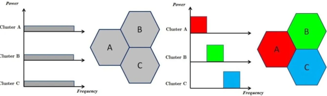
handle inter-cell interference. Because it is simple to apply to system rather than other complex settings, lots of schemes take the advantage of this concept. Reuse factor, also known as frequency reuse factor, is the number of distinct frequency sets used of a set of cells. In other word, we define n clusters, and then separate the whole frequency band into n exclusive sub-bands. Each cluster can only access the pre-assigned sub-bands. That is, a sub-band is only used by cells belonging to the same cluster. To clarify the definition of reuse factor, the concept of reuse-1 (reuse factor is 1) and reuse-3 (reuse factor is 3) is illustrated in Figure 4.

In reuse-1, every cell in the system can access the whole bandwidth with equal transmit power. Thus, we can say that there is no difference of frequency and power planning between clusters. In reuse-3, there are 3 clusters and the frequency band is separated into 3 exclusive sub-bands. Because two third of entire frequency band is forbidden to use, we can take the power which used in the forbidden frequency band to the pre-assigned sub-band. Thus each cluster can use triple transmit power in the pre-assigned sub-band to enhance the UE channel quality.

With a smaller reuse factor, more available resources can be used by a cell. According to this concept, reuse-1 must be the desirable reuse factor to be adopted in the system. But reuse-1 will cause severe interference to users located at cell edge area, thus scale the cell coverage down. Reuse-3 is proposed to overcome the problem that occurred in reuse-1, but the available resources can be obtained by a cell is only one third of reuse-1. To sum up, reuse-1 can achieve high system throughput at the cost of cell coverage; reuse-3 can achieve high cell coverage at the cost of cell capacity. To find a scheme that cannot only improve cell-edge performance but also retain the system spectrum efficiency, there are some solutions and performance discussion have been proposed [9]-[14]. Most of these solutions are based on Soft Frequency Reuse (SFR) [15], like [9], and Fractional Frequency Reuse (FFR) [16], like [10] and [11]. We will discuss these methods in the following sections.

(16)

15

Figure 4 - The frequency and power planning of reuse-1 (le ft) and reuse-3 (right). In reuse-1, a ll cells can use the entire frequency band. In reuse-3, each cell can only use one third of entire frequency band.

2.1 Resource Allocation Schemes

Before talking about different interference coordination scheme, we must have some background knowledge of resource allocation schemes. There are three common resource allocation schemes Round Robin, Max C/I and Proportional Fairness (PF) [17][18] that are applied in different interference coordination scheme. The concepts of these three schemes are briefly discussed in the following paragraphs. Noted that both RB and resource terms are being exchangeablely used in this thesis.

Assume there are N UEs in an eNB. In Round Robin scheme, every UE has the same priority to get resources. The resources are allocated to UEs in a cyclical way regardless of the channel condition of UE. Let denotes the set of RBs that were already allocated to UE i. Then a new RB will be allocated to UE k by the following formula:

(1)

Max C/I scheme considers the maximization of the system performance and not considers any fairness. Therefore, a RB will be allocated to the UE with the best channel quality. Let denotes the channel quality of each UE to RB i. Then RB i will be allocated to UE k by the following formula:

(17)

16

PF scheme considers the fairness between users, RB will be allocated depends on the long term average data rate an UE experiences. Let denotes the instantaneous data rate of each UE to RB i, and denotes the average data rate of each UE. The allocation priority of UE j for RB i is determined by proportional fairness factor where . RB i will be allocated to UE k by the following formula:

(3)

2.2 SFR Based Schemes

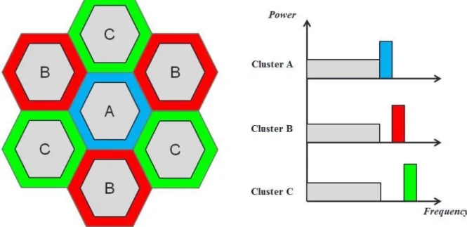
The concept of SFR is that applying reuse factor 1 at cell center area and higher reuse factor at cell edge area. In SFR, all the users are classified into two classes, one is called the cell center user (CCU) and another is called cell edge user (CEU), based on the SINR value or their distance to base station. The frequency and power planning of SFR are showed in Figure 5. The whole frequency band is divided into several parts. Number of clusters is same as the number of parts we divide. Hence, in Figure 5, the whole frequency band is divided into 3 parts and there are three clusters in the system. The CCU can use the whole bandwidth, but the CEU can only use one third of the entire frequency band. To improve data rate and cell coverage, CEU must transmit in higher power, so high power is adopted in cell edge frequency band (colored frequency band in Figure 5). For the purpose of decreasing interference from neighboring cells, the cell edge frequency bands in different cluster are disjoint.

Noted that SFR is only a frequency and power planning concept, it does not include the resource allocation scheme. If we don’t set some constrains for UEs to access the radio resource, we may not get the performance we expected. For example, CCU can access the whole frequency band, it may occupy the high power frequency band even through there are still available normal power resources. Thus, CEU may have starvation problem because the

(18)

17

high power resources are exhausted.

Based on the concept of SFR, the authors in [9] proposed a priority based interference coordination scheme named Softer Frequency Reuse (SerFR) to overcome such problem. The concept of SerFR is to set different resource access priority to CEU and CCU. For CEU, the access priority of high power frequency band is higher than normal power frequency band. For CCU, the access priority of normal power frequency band is higher than high power frequency band. In this manner, the starvation situation of CEU can be reduced.

Figure 5 - Concept of Soft Frequency Reuse scheme based on reuse factor = 3 for cell edge users and reuse factor = 1 for cell center users.

2.3 FFR Based Schemes

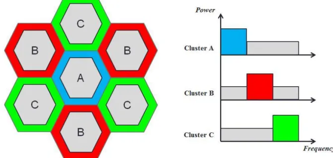
The concept of FFR is similar with SFR. It also uses two different power levels to serve CCU and CEU. In SFR, the high power frequency band of a cell is used as normal power frequency band at neighboring cells. There still has certain level inter-cell interference, especially for user located at very nearly border. For the purpose of further reducing the inter-cell interference, the high power level frequency band in FFR is totally disjoint. It means that if one cluster uses frequency band Si as high power frequency band, then the other

(19)

18

clusters are forbidden to use frequency band Si. The frequency and power planning of FFR are

showed in Figure 3. Compare to SFR, FFR sacrifices partial frequency band to enhance the signal quality that CEU experienced. Although the CCU cannot access the entire frequency band, the CEU can experience less inter-cell interference. The performance comparison of FFR, reuse-1 and reuse-3 is presented in [10]. It shows that FFR has significant improvement in both cell coverage and system throughput. The cell coverage is as good as reuse-3, which is close to 100% coverage. The system throughput is better than reuse-3 and close to reuse-1.

Figure 6 - Concept of Fractional Frequency Reuse scheme based on reuse factor = 3 for ce ll edge users and reuse factor = 1 for cell center users.

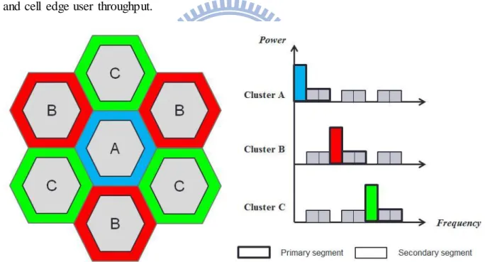
Just like SFR, FFR is also a concept of frequency and power planning. It does not include resource allocation scheme. The problem in SFR will occur in FFR, too. To conquer this problem, the authors in [11] proposed Enhanced Fractional Frequency Reuse (EFFR) based on the concept of FFR. There are three clusters in the system and power and frequency planning is illustrated in Figure 7. The whole bandwidth has been divided into three exclusive parts, and each part is assigned to a specific cluster as Primary Segment. Thus, each cluster has one third of entire frequency band as Primary Segment, the remained are called Secondary

(20)

19

high transmit power to serve CEU. According to the principle of FFR, high power frequency band of a cluster is forbidden to use in other clusters. EFFR take this advantage to set the high power as triple normal power. From a cell aspect, it looks like it takes the power of frequency band which adopts high power at other clusters to add on itself high power frequency band.

Primary Segment and Secondary Segment are defined to use in resource allocation. In resource allocation procedure, we first allocate Primary Segment to UE. Secondary Segment cannot be allocated until running out of resources in Primary Segment. In UE aspect, CEU has the higher priority to get resource than CCU. CCU can only be allocated until all the CEUs have been allocated or all the high power frequency band resources exhausted. The simulation result indicates that EFFR has better pe rformance than SFR in both cell capacity and cell edge user throughput.

Figure 7 - Concept of Enhanced Fractional Frequency Reuse scheme based on reuse factor = 3 for cell edge users and reuse factor = 1 for cell center users.

2.4 Other Inter-cell Interference Avoidance Schemes

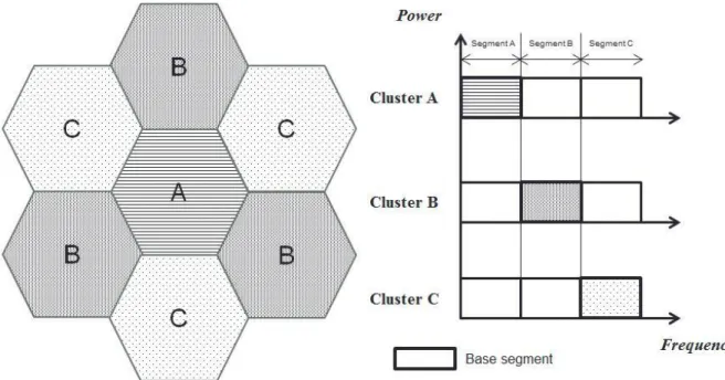
Authors in [12] proposed Incremental Frequency Reuse (IFR) Scheme. Rather than SFR and FFR, IFR does not modify the frequency and power planning. It uses the same frequency and power planning as reuse-1 for all clusters. The whole bandwidth is partitioned into several

(21)

20

exclusive parts and the number of these parts is also the number of clusters in the system. The concept of IFR is illustrated in Figure 8. Each cluster has its own base segment, which means this segment must be allocated first. For reducing inter-cell interference, the segment allocation has specific order. We take Figure 8 as an example, the segment allocation sequences can be summarized as

 Sequence-A : Segment A → Segment B → Segment C  Sequence-B : Segment B → Segment C → Segment A  Sequence-C : Segment C → Segment A → Segment B

By applying these allocation sequences, UEs in different cells have less probability to use the same frequency band, hence, inter-cell interference can be eliminated. But interference can only be eliminated when system load is not so high. When UE is getting more, system load is close to full, performance of IFR is similar with reuse-1. At this situation, UE located at cell edge cannot access the system due to low cell coverage caused by severe inter-cell interference. From the discussion above we know that IFR is only suite for light loading system. Once system loading is increasing, performance will scale down severely.

(22)

21

All of the above schemes are static in frequency domain planning. In other words, these schemes cannot adjust the bandwidth of high power frequency band and normal power frequency band while system is running. Applying these methods may bring about the user

distribution problem. If the predefined normal power frequency band is much larger than high

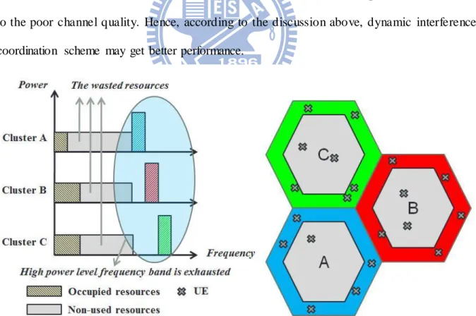
power frequency band and the user distribution is that cell edge users are much more than cell center user. Thus, some resources may be wasted because the cell edge user may not use the normal power frequency band due to the weak signal strength.

The user distribution problem is illustrated in Figure 9. The number of CEUs is more than the number of CCUs in cell A, cell B and cell C. Because the high power frequency band is too small to support CEU, some CEUs may not access the radio system. However, CCUs only occupy a little of normal power resources. There are still lots of resources remained idle. But CEUs which cannot access the radio system cannot use the normal power resources due to the poor channel quality. Hence, according to the discussion above, dynamic interference coordination scheme may get better performance.

Figure 9 - If the a mount of cell edge user is large and the a mount of cell c enter user is sma ll, some ce ll edge users may not get enough resource. Although there are id le resources, cell edge user cannot access these resources due to the bad channel quality.

(23)

22

Here we introduce two dynamic schemes. The authors of [13] observe the performance of reuse-1 and reuse-3 with VoIP traffic and data traffic. It shows that the voice users are benefited by using reuse-3 and data traffic by using reuse-1. So a dynamic scheme named

Adaptive Frequency Reuse is proposed. The concept is that each cell can dynamically adjust

the available frequency band according to the proportion of voice users. For example, if all users are not voice user, cells are allocated the entire bandwidth, what is equivalent to reuse-1 system. On the other hand, if the proportion of voice users in the system is one (all UEs are voice user), cells are allocated one third of the whole bandwidth, what is equivalent to a reuse-3 system. In this case, the way to allocate frequency band is like reuse-3, each cluster must uses exclusive frequency band. However, this scheme does not consider the frequency spectrum efficiency. In the system with a lot of voice user, the system capacity is pretty low because the available bandwidth a cell can use is close reuse-3.

Another distributed dynamic inter-cell coordination scheme which proposed in [14] can adjust the power and frequency band while system is running. The concept of [14] is to find the dominant interferer around a cell and send power restriction request through X2 interface to restrict the interference level. Although this method can get good performance, it suffers from complicated matrix calculation during finding the dominant interferer procedure. Also, each allocation run needs messages transmission a mong cells through X2 interface. It may cost too much time to finish the above job. The realistic environment constrain make this method not so practical.

To overcome the user distribution problem occurred at static scheme, the dynamic inter-cell interference coordination scheme is desirable. And for applying the practical system we need to design a scheme with the principle of low complexity and minimal messages exchange. The objective of desirable method is to retain the advantage of FFR which has the better performance both in system throughput and the cell coverage and also solve the user distribution problem. The new method must be designed to reach two main requirements:

(24)

23

 Support flexibility in frequency domain with non-uniform user distribution.  Low system complexity and minimal messages exchange.

The first requirement is used to handle that when user distribution is various, each cell can re-configure to an appropriate frequency and power planning. The second requirement is used to suite on practical system architecture, because the high complexity algorithm with lots of complicated calculation and too many inter-cell communication messages between cells is not desirable.

(25)

24

Chapter 3 Proposed Method

The discussion about advantage and limitation of the schemes we mentioned in chapter 2 motivates us to propose a new scheme named Dynamic Fractional Frequency Reuse (DFFR). DFFR can be separated into two parts, frequency and power planning and resource allocation. Based on FFR, we may have several clusters in system. How to adjust the high power frequency band between clusters is what the first part needs to do. After the first part finishing, each cell in the system has the knowledge of the frequency and power planning according to the cluster it belongs to. Based on the results getting from part one, each cell can allocate it radio resource to its serving UE in resource allocation part without central controller’s help. System architecture of DFFR is illustrated in Figure 10.

Figure 10 - System architecture of Dyna mic Fractional Frequency Reuse. In this e xa mp le, there are three c lusters and one eNB per cluster in the system. Each e NB co llects the UE info rmation fro m measurement report and then sends that to central controller. After finishing the frequency and power adjusting procedure, central controller sends the updated frequency and power planning to each eNB according to its cluster.

(26)

25

3.1 Frequency and Power Allocation

In the frequency and power planning part, for the purpose of adjusting the high power frequency band and normal power frequency band, each cell in the system needs to know the information about the channel quality, demands and distribution of its serving UE. Such information can be acquired in eNB with the help of measurement report from UE. After finishing the information collection job, every eNB sends it to the central controller to do the adjusting procedure. For reducing the complexity, adjusting procedure is separated into two phases adjusting. First phase is cluster level adjusting; central controller finds appropriate frequency and power planning for each cluster independently. Second phase is system level adjusting; because the frequency and power planning of clusters may be against the principle of FFR that high power frequency bands of each cluster are disjoint to each other, in this phase central controller needs to adjust them to an appropriate system configuration. The detail of each phase will be discussed in the following section.

3.1.1 Operation on eNB

First we need to group UEs into two categories. CCU refers to the UE with good signal quality and CEU refers to the UE with relative poor signal quality. For defining whether a UE belongs to CCU or CEU, we use the average Signal to Interference plus Noise Ratio (SINR) value of RBs as the criterion to classify and the SINR value can be derived by

(4)

where is the normal transmit power of eNB which is the power level that reuse-1

adopted for each RB, that is where is the maximum transmit power a n eNB can support and K is the number of total RBs. is a function of distance between

(27)

26

UE and its serving eNB considering antenna gain and pathloss. is the white noise power

and is the bandwidth of a RB which is 180 kHz. I means the interference from neighboring cells. If the SINR value of a UE is larger than a predefined threshold then it can be seen as CCU. Otherwise, this UE is considered as CEU and the SINR value has to be recalculated and the transmission power will replace with where is high transmit power. can also be represented of where is the ratio of high power to normal power.

According to the SINR value we can know which Modulation and Coding Schemes (MCS) can adopt to UE then the data rate per RB can also be obtained. Thus, each eNB knows how many CEU RBs (which adopt with high transmit power) and CCU RBs (which adopt with normal transmit power) it needs, the next is to check the power constrain. Because the maximum power an eNB can use is fixed, we need to confirm that the needed power of requests is below to or equal to the maximum power by the following equation

(5)

where is the number of requested RBs of CEU in cell of cluster i and

is the number of the requested RBs of CCU. The left part means that the required power for supporting all the serving UEs’ requests. If the required power is less than or equal to the maximum power, , eNB can directly report this information to central controller. If this constrain is not satisfied, it means that eNB cannot support such number of requests. Therefore, we have to perform cell level request reduction to decrease the power consumption to satisfy the power constrain. Considering fairness between CEU and CCU, we use the following equation to reduce the requests of CEU and CCU.

(28)

27 Find Subject to (6) { 𝑖𝑓 𝑖𝑓

Here is an example of the requests reducing procedure. Assume that the eNB transmit power setting of , and are 0.8 Watt, 2.4 Watt and 40 Watt respectively, that is equals to 3. The 1st cell of cluster-A has the request of

and . Obviously the requests are too many to support because the power requirement is up to 52.8 Watt. According to equation (6) we can find , then SA,1,CEU and SA,1,CEU are updated to 11 and 17 respectively. Therefore the power

consumption is reduced to 40 Watt.

After the request reducing process, eNB sends the updated information to central controller. Here we define a resource layout index to clearly describe the information that eNB send to central controller which denotes as

(7)

where _{means the resource layout index of the} cell of i cluster. means

that if the requests from CEU and CCU does not excess the maximum power constrain, there may remain some free RBs that can be adopted with normal power to use in adjusting procedure. So if an eNB does not need to perform request reducing process then

may larger than or equal to zero. Otherwise must be zero. For example of non-zero , as the power assumption of above, the 2nd cell of cluster-B has the request of and . From equation (5) we know that there will

(29)

28

remain 10 normal power RBs. Hence, and . Resource layout index can also be seen as a frequency-power mask, means that there are 10 high power RBs and 20 normal power RBs where ten of them are remained available for adjusting procedure.

3.1.2 Cell Level Adjusting

Now the central controller has the resource layout index of all the eNBs in the system. With this information, central controller can find the appropriate frequency-power mask for each cluster. The criterion is to find a frequency-power mask with minimum capacity loss among one of the frequency-power masks of this cluster. The definition of capacity loss is

(8)

It means that if a frequency-power mask of a cell is adopted for this cluster, for other same cluster eNBs, how many requests will be discarded.

Here’s a simple example. Let , and

, according to equation (5) we get that , and . This shows that using frequency-power mask of the 3rd cell of cluster C has the minimum capacity loss, so we choose as the frequency-power mask of cluster C.

After deciding all the clusters’ frequency-power mask, the phase one job is done and system level configuration starts to perform.

3.1.3 System Level Adjusting

Because the spirit of FFR is that let the high power frequency band of each cluster totally disjoint, that is, the high power frequency band of one cluster is forbidden to use in other

(30)

29

cluster. So we must ensure that the frequency-power mask of these clusters won’t overlap. Thus, for each cluster k we use the following condition to make sure if there is an overlap situation.

(9)

In equation (9), T is the set of clusters. The first term is the number of forbidden RBs because the other clusters are using. The second is the number of forbidden RBs due to itself high power frequency band. It is because, taking advantage from the concept of EFFR, using one CEU RB has to sacrifice CCU RBs. The last term can be seen as free space to adjust. From aspect of a cluster, we can say this condition is used to confirm its high power frequency band part is totally disjoint with the other clusters. If all clusters satisfy this condition, then the frequency-power mask of all the clusters won’t overlap with each other. It means that this configuration can be accepted to the system right now. Otherwise, Conflict happens and the frequency-power masks of all the clusters need to be adjusted. The system

level request reduction procedure is defined by

Find Subject to for each (10) { if if

Here is an example to show how this adjusting procedure works. Assume that there are three clusters {A, B, C} in the system and _{is 3. After the first phase done, the}

(31)

30

frequency-power masks of them are , and .

According to equation (9), it is obvious that A and B satisfy the condition but C does not. Applying the reducing process (10) we can get that , and . Hence, the updated frequency-power mask of three clusters are

, and .

Notice that during the procedure of finding , we may find more than one solution combination that can satisfy the condition. Thus, we have to choose one of them as the final solution. Because the performance won’t change variously even if we choose different solutions, so that in this part we randomly select one among the available solutions. Finally central controller ends the phase two job by sending this information to each eNB according its cluster. The final frequency-power mask of the system is shown in Figure 11.

Figure 11 - The system frequency-power configuration after frequency and power allocation part of DFFR.

(32)

31

part is done by each eNB and the second part is done by central controller. The following is the short description about each part job and pseudo code.

At eNB

a) Each eNB in the system collects the information reported from its serving UEs to decide how many high power RBs and normal power RBs it needed.

b) Each eNB adjusts the requests if it does not satisfy the power constrain. Then sends the resource layout index to central controller.

Figure 12 - Pseudo code of frequency and power allocation at eNB

At Central Controller

For each eNB

Input: N : number of serving UEs K: number of total RBs

di: demand of UEi, i = 1,2,…,N

qi,n: SINR value of UE i adopting normal power RB

qi,h: SINR value of UE i adopting high power RB

Qth: threshold between CEU and CCU

α: ratio of high power to normal power 1: PTx,norm al = Pm ax/K;

2: PTx,high = αPm ax/K;

3: SCCU = 0, SCEU = 0, Savailable = 0;

4: for i ←1 to N

5: if ( Rate(qi,n)≧Qth )

// Rate() is mapping function from SINR value to data rate 6: SCCU = SCCU + Rate(𝑞_𝑖,𝑛)/𝑑_𝑖 ;

7: else

8: SCEU = SCEU + Rate(𝑞_𝑖,ℎ)/𝑑_𝑖 ;

9: if (Si,j,CEU × PTx,high + Si,j,CCU × PTx,normal > Pm ax)

10: using equation (6) to adjust and update SCCU and SCEU

11: Savailable = K – SCCU - αSCEU;

(33)

32

a) For each cluster, choose a frequency-power mask among eNBs which belong to this cluster with minimum capacity loss as the frequency-power mask. This is the phase one job which denotes as Cluster Level Adjusting in 3.1.2.

b) Check whether the frequency-power mask between clusters will conflict or not. Performing the frequency-power mask adjusting procedure if conflict occurred. Then send the final configuration to eNBs according to their clusters. This is phase two job which denotes as System Level Adjusting in 3.1.3.

Figure 13 - Pseudo code of frequency and power allocation at central controller

3.2 Resource Allocation

In the resource allocation part we give the CEU higher priority to access the radio For central controller

Input: T : number of total clusters

NTi: number of eNB in cluster i, i = 1,2,...T

CLi,j: capacity loss of jth eNB of cluster i

ui,j: resource layout index of jth eNB of cluster i

Ui: resource layout index of cluster i

adjust: need to adjust if this value is 1; otherwise, it is 0 1: for i ← 1 to T

2: for j ← 1 to NTi

3: calculate CLi,j by equation (8);

4: k = arg minj (CLi,j);

5: Ui = ui,k;

6: for i ← 1 to T

7: using equation (9) to check collision 8: if (collision happened)

9: adjust = 1;

10: if (adjust)

11: using equation (10) to adjust and update Ui

(34)

33

resource than the CCU. It means that we further separate the resource allocation part into two steps. The first step is for CEU and the second is for CCU. At each step, we can adopt the existing resource allocation schemes we mentioned in chapter 2, which is Round Robin, Max C/I and PF. Resource allocation part can be done in following steps:

a) Allocate the high power RBs to CEU till high power RBs are exhausted or no more CEU needs resources.

b) If there were remained high power RBs can be used, allocated to CCU with relatively bad channel quality. Then allocated the normal power RBs to CCU till normal power RBs are exhausted or no more CCU needs resources.

Notice that this part is done by each eNB itself without the help of central controller. The central controller is only in charge of frequency and power allocation.

(35)

34

Chapter 4 Simulation Results

In this chapter we evaluate the performance of DFFR by simulation. We consider two tier interference sources, that is, for a cell there are two circles of neighboring cells around itself. So the system layout is set with 19 hexagonal cells and each cell equips with omni-antenna. These cells consist of three clusters which are 7 cluster-A cells, 6 cluster-B cells and 6 cluster-C cells respectively. The cell arrangement is illustrated in Figure 14.

Figure 12 - Simu lation system layout with 19 he xagonal cell which consist of 7 cluster-A ce lls, 6 c luster-B cells and 6 cluster-C cells

Because DFFR is proposed to not only to reduce the inter-cell interference from neighboring cells but also to overcome the user distribution problem, we will compare the

(36)

35

effect with EFFR with different proportion of high power sub-band to normal power sub-band to evaluate the performance. The performance is evaluated by outage network probability, resource utilization efficiency and average CEU throughput. Outage network probability and

Resource utilization efficiency are defined by (11) and (12) respectively. is the number of users cannot access the radio system and is the number of all users in the system.

and is the number of allocated RBs and number of all the RBs respectively.

(11)

(12)

We mainly focus on these two indices. Because these two indices are used to indicate the situation we mentioned in chapter 2.3 (Figure 9). In this situation, there are a lot of CEUs cannot access the system so that the network outage probability is very high. However, the high network outage probability does not cause by too many users in the system. It is because the CEU cannot access the normal power RBs due to the poor channel quality. Hence, lots of idle normal power RBs cut down the resource utilization efficiency. In this case, we expect the proposed DFFR to increase resource utilization efficiency and cut down network outage probability. That is, network outage probability only rises until resources are exhausted.

As mentioned in chapter 3, we use the SINR value as the criterion for grouping UEs. Based on the equation (13) we can derive a SINR to data rate mapping table [19].

(13)

(37)

36

QPSK (1/2) or 64-QAM (3/4)) and is the number of symbols per slot can carry on. is the number of slots per TTI and is the number of subcarriers per RB. Recall the resource block structure in chapter 1.2, RB size is determined by number of slots per TTI. In our simulation, there are two slots in a TTI. Thus we can derive Table 1.

Therefore, by looking for Table 1 we can find the achievable data rate per RB for a UE. Hence, with the UE demand we can know how many RBs it needs. For example, if a UE’s minimum required data rate is 200 kbps and the MCS it can use is QPSK (1/2), then it needs two RBs to achieve the target rate.

Table 1 - The SINR to data rate per RB mapping table

Minimum Required SINR Value (dB)

Modulation and Coding Scheme Data Rate (kbps) 1.7 QPSK (1/2) 168 3.7 QPSK (2/3) 224 4.5 QPSK (3/4) 252 7.2 16-QAM (1/2) 336 9.5 16-QAM (2/3) 448 10.7 16-QAM (3/4) 504 14.8 64-QAM (2/3) 672 16.1 64-QAM (3/4) 756

In our simulation we defined the threshold between CEU and CCU as the least SINR value that UE can apply QPSK (1/2) which is 1.7dB according to Table 1. It means that if the SINR value of an UE is less than 1.7dB, then it belongs to CEU. Otherwise, it belongs to CCU. For comparison with EFFR, we apply as 3 and the other system settings of EFFR are same as DFFR. Other simulation parameters are listed in Table 2.

(38)

37

Table 2 - Simulation parameter list

Parameter Value

Cellular layout Hexagonal grid, 19 cells

Cell range 1000m

Carrier frequency 2000MHz

System bandwidth 10MHz

BS max Tx Power 46dBm

BS antenna gain 15dBi

BS antenna height 30m

Resource block size 180KHz, total: 50 RBs

Thermal noise -174dBm/Hz

Pathloss model 122.7+35.2log₁₀(𝑑) 3

MCS

QPSK (1/2、2/3、3/4) 16 QAM (1/2、2/3、3/4)

64 QAM (2/3、3/4)

Notation of EFFR[x:y] means that the proportion of CEU RBs to CCU RBs is x:y. Notice that the CEU RBs has to further divide into each cluster, each cell got only one third of CEU RBs due to we use 3 clusters in the simulation. For example, EFFR[9.6:0.4] in Figure 15 denotes that each cell has CEU RBs and CCU RBs. Because the user distribution problem is the mainly problem we focus on, so we consider the situation similar with Figure 9 first.

In Figure 15, the UE distribution is CEU:CCU=8:2 in each cell. We observe that the outage network probability of EFFR[9.6:0.4] is close to DFFR. It is because DFFR can adjust CEU RBs and CCU RBs according to the UE distribution during the frequency and power allocation part, the simulation results may close to EFFR with appropriate proportion of CEU RBs to CCU RBs. With inappropriate proportion, see the curve of EFFR[4.2:5.8], the outage network probability increases dramatically when number of UEs is less than 50. The reason is that there are only 7 CEU RBs to allocate to CEU. Once there are more CEUs, they cannot access the system because CEU RBs exhausted. Although there are a lot of available CCU

(39)

38

RBs, they cannot access due to the poor channel quality. To put Figure 15 and F igure 16 together, we can see that EFFR with wrong RB proportion will cause high outage network probability and low resource utilization efficiency. This result indicates that lots of RBs are wasted. For example, notice that the case of 20 UEs which is circled in red in Figure 15 and Figure 16, the outage network probability of EFFR[4.2:5.8] rises to about 46% and the resource utilization efficiency is only 31%. Compare with EFFR[9.6:0.4] and DFFR, outage network probability is less than 10% and resource utilization efficiency is about to 100%.

Notice that the outage network probability of EFFR[4.2:5.8] is less than DFFR and EFFR[9.6:0.4] when number of UE is over 60, it does not means the former got better performance. The reason is that the number of total available RBs in these three schemes is different. DFFR is similar with EFFR[9.6:0.4] which has 16 CEU RBs and 2 CCU RBs per cell and EFFR[4.2:5.8] has 7 CEU RBs and 29 CCU RBs per cell. In the case of 20 UEs, there are about 4 CCUs and 16 CEUs. In this situation DFFR and EFFR[9.6:0.4] are out of resources because all the CCU RBs and CEU RBs are allocated to UEs. Hence, if there are more UEs coming, no more resources can be allocated, outage network probability rises. EFFR[4.2:5.8] has much more available RBs than DFFR and EFFR[9.6:0.4]. So when number of UEs comes to 60, it still has CCU RBs to allocate to CCU. However, at the CEU aspect, see Figure 17, average CEU throughput of EFFR[9.6:0.4] and DFFR is much higher than EFFR[4.2:5.8]. From these results we can observe that when number of UEs getting more, it is a tradeoff between serving more CEUs and reducing the outage network probability.

(40)

39

Figure 13 - Co mparison of outage network probability between DFFR and EFFR with different proportion in case of CEU:CCU=8:2 UE distribution.

Figure 146 - Co mparison of resource utilization effic iency between DFFR and EFFR with different proportion in case of CEU:CCU=8:2 UE distribution.

(41)

40

Figure 15 - Comparison of CEU average throughput between DFFR and EFFR with different proportion in case of CEU:CCU=8:2 UE distribution.

To further confirm that DFFR has the similar performance with EFFR with appropriate proportion of CEU RBs to CCU RBs, we choose another case to test again. Considering the UE distribution of half CEU and half CCU, we compare with EFFR with different proportion of CEU RB to CCU RB to see outage network probability and resource utilization efficiency. In EFFR[7.2:2.8], each cell has 12 CEU RBs and 14 CCU RBs, it is close to the proportion of half CEU to half CCU. As we expected, Figure 18 shows that DFFR has nearly the same curve as EFFR[7.2:2.8]. Both of them have better performance in outage network probability. Especially in the case of 30 UEs, the difference DFFR and EFFR[7.2:2.8] is up to 25%. From Figure 19 we can see that although resource utilization efficiency of EFFR[9.6:0.4] is higher than both DFFR and EFFR[7.2:2.8] when UE less than 30, the outa ge network probability of the former is higher than the latter two. It is because the total available RBs of EFFR[9.6:0.4] is less than EFFR[7.2:2.8] and DFFR. Once any RB being allocated, resource utilization

(42)

41

efficiency raise up rapidly. This is also the reason that EFFR[9.6:0.4] has higher outage network probability, because all the resources exhausted when number of UEs is over than 20.

Figure 168 - Comparison of outage network proportion between DFFR and EFFR with different proportion in case of CEU:CCU=5:5 UE distribution.

Figure 179 - Comparison of resource utilization efficiency between DFFR and EFFR with different pro portion in case of CEU:CCU=5:5 UE distribution.

(43)

42

Chapter 5 Conclusion and Future Work

In this work, we proposed a fractional frequency reuse-based inter-cell interference avoidance method named DFFR. Considering reducing complexity, other than collecting the whole system UEs’ information to central controller, we divide the frequency and power allocation process into two phase job. Also, we focus on the problem caused by different user distribution. With different user distribution, DFFR can adjust the frequency and power allocation before allocating resources to UEs. Thus, applying DFFR can prevent the waste of resources due to inappropriate proportion of CEU RBs to CCU RBs. By the simulation results, we proved that this approach efficiently reduced the outage network probability and increase resource utilization efficiency. We also observe that there is a tradeoff between serving more CEUs and reducing outage network probability when number of UEs is increasing. Because we must sacrifice CCU RBs for serving CEU, hence the total available RBs are reduced and outage network probability rises rapidly.

However, DFFR considers only two different power levels. If there are several power levels, we can further group UEs into different groups. With the power diversity, the sacrificed resources can be reduced; the tradeoff between outage network probability and serving more CEUs can be relaxed. Therefore, adopting several power levels will be study in the following work.

(44)

43

References

[1] S. Sesia, I. Toufik and M. Baker, LTE - The UMTS Long Term Evolution：From Theory

to Practice, John Wiley & Sons, Ltd. 2009.

[2] W. Mohr, “The WINER (Wireless World Initiative New Radio) Project - Development of a Radio Interface for Systems Beyond 3G,” International Journal of Wireless Information

Networks, vol. 14, no.2, pp. 67-78, June 2007.

[3] IEEE Standard for Local and Metropolitan Area Networks Part 16: Air Interface for

Broadband Wireless Access Systems, IEEE Standard 802.16, 2009.

[4] H. Holma and A. Toskala, LTE for UMTS - OFDMA and SC-FDMA Based Radio Access, John Wiley & Sons, Ltd. 2009.

[5] J. G. Andrews. (2005. Apr.). Interference Cancellation for Cellular Systems: A Contemporary Overview, IEEE Wireless Communication Magazine, pp. 19-29. [6] Physical layer aspects for Evolved UTRA, 3GPP TR 25.814, Sept. 2006.

[7] Evolved Universal Terrestrial Radio Access (E-UTRA) and Evolved Universal Terrestrial

Radio Access Network (E-UTRAN) Overall description Stage 2, 3GPP TS 36.300, March

2010.

[8] G. Boudreau, J. Panicker, N. Guo, R. Chang, N. Wang, and S. Vrzic. (2009. May 5) Interference Coordination and Cancellation for 4G Networks, IEEE Communications

Magazine, pp. 74-81.

[9] X. Zhang, C. He, L. Jiang and J. Xu, “Inter-cell Interference Coordination Based on Softer Frequency Reuse in OFDMA Cellular Systems,” in Proc. IEEE International

Conference on Neural Network and Signal Processing, ICNNSP’08, Zhengjiang, China, 7-11

June 2008, pp. 270-275.

[10] A. Lodhi, A. Awad, T. Jeffries and P. Nahi, “On Re-use Partitioning in LTE-FDD Systems,” in Proc. IEEE Personal, Indoor and Mobile Radio Communications Conference,

PIMRC’09, Tokyo, Japan, 13-16 Sept. 2009, pp. 910-913.

(45)

44

High Spectral Efficiency in OFDMA,” in Proc. IEEE Wireless Communications and

Networking Conference, WCNC’10, Australia, Syndney, 18-21 April 2010. pp. 1-6.

[12] K. T. Kim and S. K. Oh, “An Incremental Frequency Reuse Scheme for an OFDMA Cellular System and Its Performance,” in Proc IEEE Vehicular Technology Conference,

VTC’08, Singapore, 11-14 May 2008, pp. 1504-1508.

[13] Z. Bakhti and S. S. Moghaddam, “Inter-Cell Interference Coordination with Adaptive Frequency-Reuse for VoIP and Data Traffic in Downlink of 3GPP-LTE,” in Proc IEEE

International Conference on Application of Information and Communication Technologies, ICAICT’10, Tashkent, Uzbekistan, 12-14 Oct. 2010, pp. 1-6.

[14] M. Rahman, H. Yanikomeroglu and W. Wong, “Interference Avoidance with Dynamic Inter-Cell Coordination for Downlink LTE System,” in Proc IEEE Wireless Communications

and Networking Conference, WCNC’09, Budapest, Hungary, 5-8 April 2009. pp. 1-6.

[15] Huawei, “Soft Frequency Reuse Scheme for UTRAN LTE,” Athens, Greece, R1-050507, 9-13 May 2005.

[16] Siemens, “Interference Mitigation by Partial Frequency Reuse,” Denver, USA, R1-060670, 13-17 Feb. 2006.

[17] H. Kim, K. Kim, Y.Han and S. Yun, “A Proportional Fair Scheduling for Multicarrier Transmission Systems,” in Proc. IEEE Vehicular Technology Conference, VTC’04, Vol. 1, Los Angeles, CA, 26-29 Sept. 2004. pp. 409-413

[18] P. Chang, Y. Chang, Y. Han, C. Zhang, D. Yang, “Interference Analysis and Performance Evaluation for LTE TDD System,” in Proc. IEEE International Conference on Advanced

Computer Control, ICACC’10, Vol. 5, Shenyang, China, 27-29 March 2010. pp. 410-414

[19] K. Sandrasegaran, H. A. Mohd Ramli and R. Basukala, “Delay-Prioritized Scheduling (DPS) for Real Time Traffic in 3GPP LTE System,” in Proc IEEE Wireless Communications

and Networking Conference, WCNC’10, Australia, Syndney,18-21 April 2010, pp. 1-6.

長程演進網路下載系統基於部分頻率複用之協同式干擾避免機制