隨機波動度下選擇權訂價模型之參數估計與實證分析:以台灣市場為例

全文

(1)國立交通大學財務金融研究所碩士論文. 隨機波動度下選擇權訂價模型之參數估計與實證分析: 以台灣市場為例. Estimation and Empirical Performance of a Stochastic Volatility Option-Pricing Model: the Case of the Taiwan Market. 研究生：楊華勝指導教授：李昭勝教授中華民國九十三年六月.

(2) 隨機波動度下選擇權訂價模型之參數估計與實證分析: 以台灣市場為例 Estimation and Empirical Performance of a Stochastic Volatility Option-Pricing Model: the Case of the Taiwan Market 研究生：楊華勝. Student: Hua-Sheng Yang. 指導教授：李昭勝教授. Advisor: Dr.Jack C. Lee. 國立交通大學財務金融研究所碩士論文. A Thesis Submitted to Institute of Finance College of Management National Chiao Tung University in partial Fulfillment of the Requirements for the Degree of Master in Finance June 2004 Hsinchu, Taiwan, Republic of China. 中華民國九十三年六月.

(3) 隨機波動度下選擇權訂價模型之參數估計與實證分析: 以台灣市場為例. 研究生：楊華勝. 指導教授：李昭勝教授. 國立交通大學財務金融研究所. 摘要這篇論文檢驗由 Heston(1993)所提出的隨機波動度的選擇權訂價模型在台灣市場的表現。我使用馬可夫鍊蒙地卡羅的方法去估計該模型的參數。我也探討了隨時間變化的偏態係數與峰態係數對此模型表現之潛在的影響。我發現到此模型傾向高估價外的買權和低估價內的買權。此外，每日的波動度之風險報酬有隨著時間而波動的表現；然而證據和分析顯示波動度之風險報酬對 Heston 的選擇權訂價模型沒有影響。. i.

(4) Estimation and Empirical Performance of a Stochastic Volatility Option-Pricing Model: the Case of the Taiwan Market. Student: Hua-Sheng Yang. Advisor: Dr. Jack C. Lee. Institute of Finance National Chiao Tung University. Abstract This thesis examines the stochastic volatility option pricing model suggested by Heston (1993) in Taiwan Market. I employ Markov chain Monte Carlo method to estimate the model parameters. I also discuss the potential effect of time-varying skewness and kurtosis on the performance of the model. It is found that the model tends to overprice out-of-money calls and underprice in-the-money calls. Moreover, the daily volatility risk premium shows a volatile behavior over time; however, the evidence suggests that the volatility risk premium has a negligible impact on the pricing performance of Heston’s model.. ii.

(5) Acknowledgements 首先要感謝我的指導教授李昭勝老師，在這二年給予我細心的指導，也要感謝統計所博士班的牛維方學長，總是不厭其煩地給予我幫助與建議，讓這篇碩士論文可以順利的完成；此外，感謝資科所的曾昆南同學，幫助我克服寫程式時遇到的難題。感謝我碩士班的同學和研究團隊的伙伴們，陪伴我在求學的路上一起成長，也謝謝應數系籃球隊的學弟們，陪伴我打球與連誼，讓我身心健康的渡過這二年。當然我的父母讓我無憂慮地求學與背後的支持更是一大支柱，僅將這篇論文，獻給我最敬愛的父母。. iii.

(6) Contents Chinese Abstract English Abstract Acknowledgements Contents List of Tables List of Figures 1 2 3. i ii iii iv v vi. Introduction Heston's Stochastic Volatility Option Pricing Model Estimation of the Diffusion Parameters 3.1 The MCMC Algorithm ……………………………………………………. 1 5 7 7. 3.2 Estimating Instantaneous Variance ……………………………….……… 3.3 Simulation Results …………………………………………………..……. 9 10. 4. The Taiwan TAIEX Index Options 4.1 Market Description ………………………………………………..……… 4.2 The Data ……………………………………………………………..……. 11 11 13. 5 6. Empirical Results Estimating the Implied Variance and the Volatility Risk Premium 6.1 Estimation Procedure ………………………………………………..…… 6.2 The Volatility Risk Premium ………………………………………..…… 6.3 Implied Volatility Graphs …………………………………………………. 15 19 19 21 22. 7. Out-of-sample Pricing Performance 7.1 Out-of-sample Pricing Error ……………………………………………… 7.2 Skewness and Kurtosis ……………………………………………………. 25 25 28. 8. Conclusions. 31. Appendix A Heston's Stochastic Volatility Option Ppricing Formula Appendix B Posterior Distributions for Volatility Appendix C (Un)conditional skewness and kurtosis. 33 34 35. References. 36. iv.

(7) List of Tables 1 2 3 4 5. Simulation results for Heston's model ……………………………………………… Sample characteristics of TAIEX index options …………………………………… Summary statistics for the continuously compounded returns ……………………… TAIEX parameter estimates ………………………………………………………… Out-of-sample pricing errors ………………………………………………………. v. 10 14 16 16 27.

(8) List of Figures 1 2 3 4 5 6 7 8 9. Time plot of the daily TAIEX index ……………………………………………… Estimated Volatility paths and realized volatility for the TAIEX index …………… MCMC estimates from September 2003 to December 2003 ………………………… Daily volatility risk premium for MCMC variance estimate ………………………… Daily volatility risk premium for implied instantaneous variance …………………… Daily implied volatilities …………………………………………………………… Smiles ……………………………………………………………………………… Time-varying skewness …………………………………………………………… Time-varying kurtosis ………………………………………………………………. vi. 15 17 18 20 22 24 24 30 30.

(9) 1. Introduction. Since Black and Scholes (1973, henceforth BS) and Merton (1973) originally developed their option valuation formulas, literally hundreds of papers have been written on the valuation of derivatives securities such as options on different underlying assets, forward contracts, futures contracts, swaps, and so forth. After the crash in 1987, the implied volatility of options has often been found to be decreasing and convex in the exercise price. There have been various attempts to deal with this apparent failure of the BS formula and researchers have developed option valuation models that incorporate stochastic volatility. Traditionally, volatility dynamics in asset prices have been explored using the time series of returns on the assets being studied. Following the work of Engle (1982) and Bollerslev (1986), the discrete-time Generalized Autoregressive Conditional Heteroskedasticity (GARCH) models have been studied extensively for this purpose and remain popular today. Because of the rapid growth in derivatives markets, the continuous-time stochastic volatility models have recently become popular as well. The continuous-time stochastic volatility models of Hull and White (1987), Scott (1987), Wiggins (1987) and Heston (1993) are the key extensions of the BS model. Bates (1996) and Bakshi, Cao and Chen (1997) further develop the stochastic volatility model suggested by Heston (1993) in order to account for both stochastic jumps and interest rates. It should also be noted that Heston (1993) provides a closed-form solution for the European call option without imposing the restrictions of zero correlation and zero price of volatility risk by using Fourier inversion methods. While the model is written in continuous time, the available data are always sampled discretely in time. Ignoring the difference can result in inconsistent estimators (see, e.g., Merton (1980) and Melino (1994)). A number of econometric methods have been recently. 1.

(10) developed to estimate the parameters of the continuous-time stochastic volatility models, without requiring that a continuous record of observations be available. Some of these methods are based on the generalized method of moments (Hansen and Scheinkman (1995), Duffie and Glynn (1997), Kessler and Sorensen (1999)), others are on the simulations. Duffie and Singleton (1993) provide a procedure for obtaining simulated moments estimators that are consistent and asymptotically normal. The indirect inference procedures of Gouriéroux, Monfort, and Renault (1993) and the efficient method of moments (EMM) approach proposed by Gallant and Tauchen (1996) provide convenient estimation methods. Nonparametric density-matching (Aït-Sahalia (1996a, 1996b)), nonparametric regression for approximate moments (Stanton (1997)), and Markov Chain Monte Carlo methods (Eraker (2001) and Jones (1998)) are also proposed. Sundaresan (2000) provides a comprehensive review of the development of this field. In related research, Heston and Nandi (2000) propose a closed –form GARCH model in which it is possible to value options using volatilities calculated directly from the historical sample of security returns and simplify the estimation procedure. The discussion above motivated this research. The key objective of the thesis is to evaluate the empirical performance of the stochastic volatility model proposed by Heston (1993) relative to the BS framework for the Taiwan TAIEX index options. Time-series returns on the underlying index are employed to estimate the parameters of the stochastic variance process imposed by Heston’s model. This is done using Markov chain Monte Carlo (MCMC) methods. It is an appropriate method for adjusting for the discretization biases when estimating the parameters of the continuous variance process under the true probability measure. Moreover, this approach allows us to analyze the empirical behavior of the parameters characterizing the diffusion process assumed for the instantaneous variance. Their behavior is discussed relative. 2.

(11) to the appropriate skewness and kurtosis underlying in Heston’s model. This provides us with insights towards understanding the characteristics of the stochastic volatility option-pricing model. It must be pointed out that the usual cross-sectional approach employed by Bakshi, Cao and Chen (1997) to test stochastic option models may easily ignore relevant information in the original series that may not be embedded in the option prices. Since the risk-neutral and objective measures are not wholly dissimilar, there must be an advantage to using both sets of the time series of the underlying’s prices and the prices of options on it to infer both measures simultaneously, a point made forcefully by Chernov and Ghysels (2000). The approach proposed in the thesis enables us to combine the cross-sectional information in options with the information contained in the time series returns of the underlying security. The estimation procedure has two separate steps. First, I estimate the parameters of the stochastic volatility , which are required inputs for Heston’s model, by employing the MCMC estimation technique on a time-series of the underlying hourly returns. Second, the price of the volatility risk and the instantaneous variance are obtained by minimizing the sum of squared pricing errors between the option model and market prices as in Bakshi, Cao and Chen (1997). Then theoretical prices are obtained for alternative specifications of Heston’s model and compared with BS option prices. Fiorentini, León, and Rubio (2002) have found that the model tends to overprice out-of-the-money calls and underprice in-the-money calls in a thinly traded market. Moreover, they suggest that the volatility risk premium has a negligible impact on the pricing performance of Heston’s model. The overall empirical evidence regarding the behavior of the volatility risk premium will be discussed in this thesis. The rest of the thesis proceeds as follows. Section 2 introduces the theoretical model employed in this thesis, and Section 3 describes the approaches for estimation. In Section 4 I. 3.

(12) give a brief summary of the Taiwan TAIEX index options market and data. Section 5 summarizes the empirical results regarding the time series estimation of the stochastic volatility parameters and Section 6 provides the implied volatility graphs and the estimation of the volatility risk premium through option prices. I analyzes the out-of-sample option pricing performances in Section 7. Section 8 concludes.. 4.

(13) 2. Heston’s stochastic volatility option-pricing model. By far the most popular recent formulations of stochastic volatility in continuous time have been variants of the stochastic volatility model of Heston (1993). Heston obtains a closed-form solution for price of a European call option on an asset with stochastic volatility. He works with Fourier transforms of conditional probabilities that the option expires in-the-money. The characterization of these probabilities is achieved through their characteristic function. Using a square root process to represent the dynamics of instantaneous variance, Heston assumes the processes dSt = µ St dt + Vt St dW1t , dVt = κ (θ − Vt ) dt + σ Vt dW2t ,. (1). dW1t dW2t = ρ dt ,. where µ is the instantaneous expected rate of return of the underlying asset, Vt is the instantaneous stochastic variance, θ is the long-term mean of the variance, κ governs the rate at which the variance converges to this mean, and σ represents the volatility of the variance process. The parameters of the variance process, θ , κ , and σ are all strictly positive constants. W1t. and W2t. are standard Brownian motions allowed to be. instantaneously correlated. Thus, increases or decreases in volatility could be related to the level of the underlying asset. For option pricing, much interest centers around the values of κ , σ , and ρ , which determine the ways in which the distribution of St departs from the lognormality. Kurtosis depends in large part on the magnitude of σ relative to that of κ . If σ is relatively large, more “volatile” variance will lead to fat tails, raising the prices of all options far from at-the-money. Skewness depends in addition on ρ , and it has often been argued that the 5.

(14) typical downward slope of Black-Scholes implied volatilities of equity options across moneyness (the leverage effect) is evidence of a negative value of ρ . The risk-neutral probability measure incorporates the market price of volatility, denoted as. λ , to distinguish the objective probability measure from the risk-neutral one. The volatility risk premium is assumed to be proportional to the instantaneous variance, λVt , and its sign arises from the sign of correlation between the Brownian motions assumed for the instantaneous variance and the aggregate consumption. The risk-neutral version model is given by: dSt = rSt dt + Vt St dW1∗t ,. dVt = κ ∗ (θ ∗ − Vt ) dt + σ Vt dW2∗t ,. (2). dW1∗t dW2∗t = ρ dt ,. where κ ∗ = κ + λ , θ ∗ = κθ (κ + θ ) . Let c ( S , v, t ) be the value of a European call option where S ≡ St and v ≡ Vt to abbreviate. Heston’s formula is given by: c ( S , v, t ) = St P1 − e. − r (T − t ). KP2 ,. (3). where P1 and P2 are two risk-neutralized probabilities having the same interpretation as in the standard BS expression. The formulae are provided in Appendix A.. 6.

(15) 3. Estimation of the diffusion parameters. 3.1. The MCMC Algorithm. This. section. develops. a. likelihood-based. estimation. approach. for. estimating. continuous-time stochastic volatility models using Markov chain Monte Carlo (MCMC) methods. Robert and Casella (1999) provide a general discussion of these methods, and Johannes and Polson (2002) provide an overview of MCMC estimation of continuous-time models. This approach has several advantages over other estimation methods. First, MCMC provides both estimates of parameters and the latent volatility. Second, MCMC accounts for the estimation risk. Third, MCMC methods have been shown in related settings to have superior sampling properties to competing methods. Jacquier, Polson, and Rossi (1994) find in simulations that MCMC outperforms GMM and QMLE in estimation of stochastic volatility models, and Andersen, Chung, and Sorensen (1999) find that MCMC outperforms EMM. Fourth, MCMC is based on conditional simulation, therefore avoiding any optimization or unconditional simulation. MCMC methods are computationally efficient so that we can check the accuracy of the method using simulations. The approach suggested here uses only time series data to estimate the models, although it can be extended in a straightforward manner to include option price data (see Eraker (2003)). Let Yt ≡ ln St , and consider the process under the original probability measure given by dYt = µ dt + Vt dW1t , dVt = κ (θ − Vt ) dt + σ Vt dW2t ,. (4). dW1t dW2t = ρ dt ,. where Θ ≡ ( µ , κ , θ , σ , ρ ) denotes the vector of parameters of interest. It should be noted that. 7.

(16) 1 the original return drift of the diffusion process of Yt , by using Ito’s lemma, is µ − Vt . 2. Eraker, Johannes, and Polson (2003) originally included a variance risk premium term in the return drift, µ + βVt . It is found this parameter insignificant in models and therefore is dropped from the analysis. I follow their point, consistent with Andersen, Benzoni, and Lund (2002) and Pan (2002), which will not affect the estimation of the parameters of the variance process and the option pricing. The basis for our MCMC estimation is a time-discretization of Eq. (4),. Y(t +1) ∆ = Yt ∆ + µ∆ + Vt∆ ∆ε (yt +1) ∆ , V( t +1) ∆ = Vt ∆ + κ (θ − Vt ∆ ) ∆ + σ Vt∆ ∆ε (vt +1) ∆ ,. (5). where ε (yt +1) ∆ and ε (vt +1) ∆ are standard normal random variables with correlation ρ and ∆ is the time-discretization interval. In this study, I set the discretization interval equals the observed frequency. The procedure could introduce a discretization bias, although the bias is typically quite small with daily data. I provide simulations below to support this claim. It should be noted that we could introduce additional unobserved data points between dates t and t + 1 to reduce any bias and treat them as missing data points to be included in the MCMC simulation (see Eraker (2001)). The posterior distribution summarizes the sample information regarding the parameters,. Θ = ( µ , κ , θ , σ , ρ ) , and the latent volatility: p ( Θ,V | Y ) ∝ p (Y | Θ,V ) p ( Θ,V ) ,. (6). where Y = {Yt }t =1 are the observed prices, V = {Vt }t =1 are the unobserved variances, and T T. T. is the sample size. The posterior combines the likelihood, p (Y | Θ,V ) , and the prior,. p ( Θ,V ) . 8.

(17) As the posterior distribution is not known in closed form, our MCMC algorithm generates samples by iteratively drawing from the following conditional posteriors:. parameters : p ( Θi | Θ− i , V , Y ) , i = 1,… , k. (. ). volatility : p Vt ∆ | V( t +1)∆ ,V( t −1)∆ , Θ, Y , t = 1,… , T , where Θ−i denotes the elements of the parameter vector except Θi . Drawing from these distributions is straightforward, with the exception of volatility, as the distribution is not of standard form. Appendix B provides the details of the posterior distributions and our choice of priors. The algorithm produces a set of draws. {Θ. (g). ,V ( g ) }. G g =1. which are samples from. p ( Θ,V | Y ) . Johannes and Polson (2002) provide a review of the theory behind MCMC algorithms.. 3.2. Estimating instantaneous variance. The MCMC approach provides a straightforward method to estimate the instantaneous variance by computing the posterior expectation of the variable. Therefore, I provide a Monte Carlo solution to the classical, latent variable estimation problem. The key is that the MCMC algorithm generates samples of the spot variance drawn from the joint posterior distribution. Given these samples, the Monte Carlo estimate of the mean of the posterior variance distribution is. E[Vt∆ | Y ] ≈. 1 G (g) ∑Vt∆ , G g =1. (7). where Vt∆( g ) is the variance at time t in the g th iteration of the algorithm. No additional calculations are required. Latent variable estimation is just a by-product of our algorithm. This estimate takes into account parameter uncertainty. To see this, note that I estimate. 9.

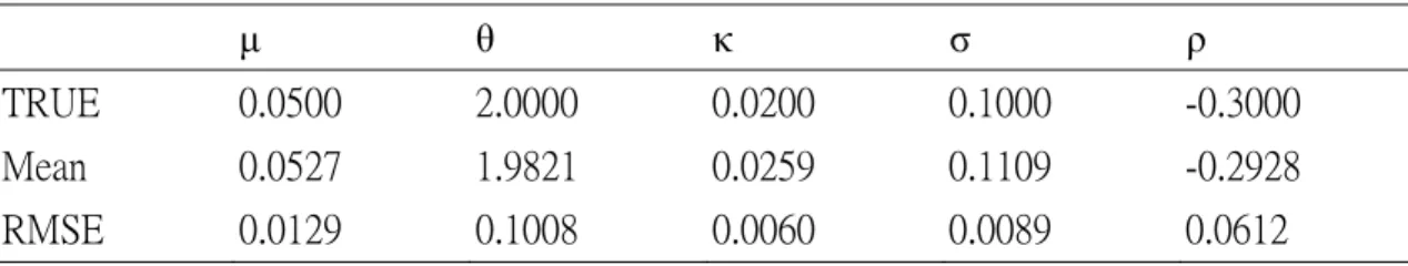
(18) E [Vt∆ | Y ] and not E [Vt∆ | Y , Θ] . The former distribution integrates out all of the parameter uncertainty. The latter distribution treats the parameter estimates as known, ignoring the fact that they are random variables.. 3.3. Simulation Results. I performed Monte Carlo simulations to check the reliability of my estimation approach. Since I time discretize the continuous-time model, it is important to check that this does not introduce any biases in parameter estimates. My simulations used 100 artificial data sets consisting of 250 data points each. The data were generated using the Euler discretization of the Heston’s model with ∆ = 1 20 . Hence, my estimation method is measured against the artificial data generated by the true continuous time process. I used a posterior sample size of 50,000 for each of the MCMC runs. Table 1 reports simulations for the Heston’s model. The table reports the means and the root mean squared error (RMSE) and the results indicate that the algorithm delivers extremely accurate estimates for most of the parameters.. Table 1: Simulation results for Heston’s model µ. θ. κ. σ. ρ. TRUE. 0.0500. 2.0000. 0.0200. 0.1000. -0.3000. Mean. 0.0527. 1.9821. 0.0259. 0.1109. -0.2928. RMSE. 0.0129. 0.1008. 0.0060. 0.0089. 0.0612. 10.

(19) 4.. The Taiwan TAIEX index options. 4.1. Market description. We begin with a brief description of the Taiwan Stock Exchange Corporation (TSEC). The Exchange maintains a total of 28 stock price indices, to allow investors to grab both overall market movement and different industrial sectors' performances conveniently. The indices may be grouped into market value indices and price average indices. The former are similar to the Standard & Poor's Index, weighted by the number of outstanding shares, and the latter are similar to the Dow Jones Industrial Average and the Nikkei Stock Average. The TSEC Capitalization Weighted Stock Index (TAIEX) is the most widely quoted of all TSEC indices. TAIEX covers all of the listed stocks excluding preferred stocks, full-delivery stocks and newly listed stocks, which are listed for less than one calendar month. Up to December 2002, 593 issues were selected as component stocks from the 638 companies listed on the Exchange. Trading on the Exchange starts at 09:00 and closes at 13:30. The orders can be entered half an hour before the trading session starts. Buy or sell orders are in standard unit or multiples of standard units. One standard trading unit is 1,000 shares, which is applicable to all listed stocks. Orders below 1,000 shares are considered odd-lot and that over 500,000 shares are block trading. Under current trading rules, the closing price of a stock is simply the last traded price of the intra-day continuous auction of the trading day. Given that the closing price of securities is widely used by market participants as a benchmark for portfolio valuation as well as index calculation, the new system will accumulate orders for 5 minutes (from 1:25 p.m. to 1:30 p.m.). 11.

(20) before the closing call auction. The TSEC imposes a 7% price limits for all traded stocks. Within a trading day, the price for a single stock cannot move more than 7% from the previous price after adjusting for dividend and stock splits. Therefore, the maximum close to close 1-day return is 7% and the minimum return is -7%. The official derivative market for risky assets, which is known as Taiwan Futures Exchange (TAIFEX), trades a future contract on TAIEX, the equivalent option contract for calls and puts, and individual option contracts for blue-chip stocks. Trading in the derivative market started in 1998. The market has experienced tremendous growth from the very beginning. Launched on December 24th, 2001, the TAIEX index options achieved a total of 1,566,446 contracts by the end of 2002, accounting for 19.72% of the market total for the year. According to Trade Data Global Services, the TAIFEX ranked 27th among exchanges worldwide in terms of trading volume of futures contracts, moving up 5 places from 2001. TAIFEX took 30th place in terms of trading volume of all products, edging up 6 places from 2001. The TAIEX option contract is a cash-settled European option with trading during the three nearest consecutive months and the other 2 months of the March quarterly cycle (March, June, September, and December). The last trading day is the third Wednesday of the delivery month and the expiration day is the first business day following the last trading day. Trading occurs from 08:45 to 13:45. During the sample period covered by this research, the contract size is 50 New Taiwan dollars times the TAIEX index, and prices are quoted in points, with a minimum price change of one-tenth point (NT$5). The exercise prices are given in 100 index point intervals in spot month, the next two calendar months and 200 index point intervals in the additional two months from the March quarterly cycle. It is important to point out that liquidity is concentrated on the nearest expiration contract.. 12.

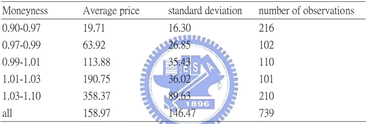
(21) Thus, during 2002 and 2003 almost 90% of crossing transactions occurred in contracts of this type.. 4.2. The data. I use the call options on the TAIEX index traded daily on TAIFEX during the period from September 1, 2003 through December 31, 2003. Given the concentration in liquidity, my daily set of observations includes only calls with the nearest expiration day. Moreover, I eliminate all transactions taking place during the last week before expiration (to avoid the expiration-related price effects). As usual in this type of research, my primary concern is the use of simultaneous prices for the options and the underlying security. The data, which are based on all reported transactions during each day throughout the sample period, do not allow us to observe simultaneously enough options with different exercise prices. In order to avoid large variations in the underlying security price, I restrict my attention to the 25-min window from 13:00 to 13:25. It turns out that on average during my sample period almost 20% of crossing transactions occur during this interval. At the same time, using data from the same period each day avoids the possibility of intraday effects. These criteria yield a final daily sample of 739 observations. Table 2 describes the sample properties of the call option prices employed in this work. Average prices, standard deviations, and the number of available calls are reported for each moneyness category. Moneyness is defined as the ratio of the spot price to the exercise price. A call option is said to be deep out-of-the money if the ratio S / K belongs to the interval. (0.90,0.97) ;. out-of-the-money (OTM) if 0.97 ≤ S / K < 0.99 ; at-the-money (ATM) when. 13.

(22) 0.99 ≤ S / K < 1.01 ; in-the-money (ITM) when 1.01 ≤ S / K < 1.03 ; and deep-in-the-money if 1.03 ≤ S / K < 1.10 . As indicated, there are 2,028 call option observations, with OTM, ATM and ITM options, respectively, accounting for 45%, 13% and 42%. The average call price ranges from 29.22 NT dollars for deep OTM options to 323.21 NT dollars for deep ITM options. To proxy for riskless interest rates, I use the daily series of annualized Taiwan deposit 1 month rates from the First Commercial Bank of Taiwan.. Table 2: Sample characteristics of TAIEX index options Moneyness. Average price. standard deviation. number of observations. 0.90-0.97. 19.71. 16.30. 216. 0.97-0.99. 63.92. 26.85. 102. 0.99-1.01. 113.88. 35.43. 110. 1.01-1.03. 190.75. 36.02. 101. 1.03-1.10. 358.37. 89.63. 210. all. 158.97. 146.47. 739. 14.

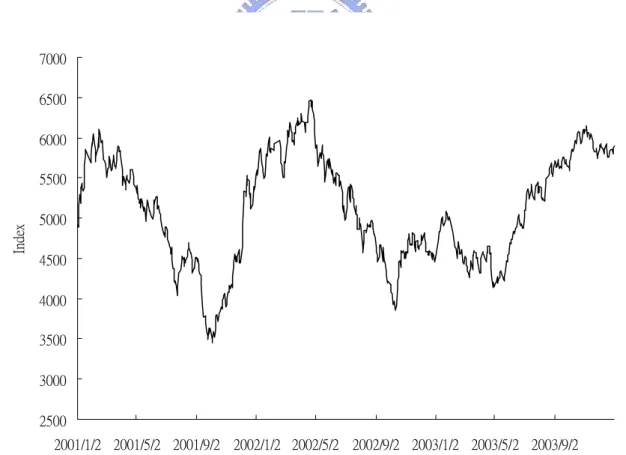
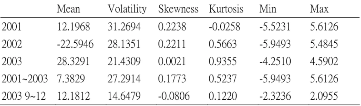
(23) 5. Empirical results. I estimate the model using TAIEX index returns from January 2, 2001 to December 31, 2003. Excluding weekends and holidays, I have 739 daily observations for the TAIEX. Figure 1 is the time plot of the daily TAIEX index and the Table 3 provides summary statistics for the continuously compounded returns, scaled by 100. Because the situations of the stock market for each year seem quite different, I also provide the estimates of the model using the daily index returns for each year. Table 4 summarizes the parameter estimation of the model for the TAIEX during 2001, 2002, 2003, and 2001 to 2003.. Figure 1: Time plot of the daily TAIEX index. 7000 6500 6000. Index. 5500 5000 4500 4000 3500 3000 2500 2001/1/2 2001/5/2 2001/9/2 2002/1/2 2002/5/2 2002/9/2 2003/1/2 2003/5/2 2003/9/2 Date. 15.

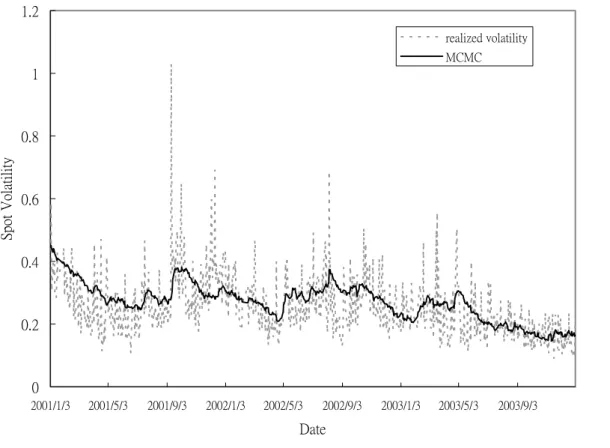
(24) Table 3: Summary statistics for the continuously compounded returns Mean. Volatility. Skewness Kurtosis. Min. Max. 2001. 12.1968. 31.2694. 0.2238. -0.0258. -5.5231. 5.6126. 2002. -22.5946. 28.1351. 0.2211. 0.5663. -5.9493. 5.4845. 2003. 28.3291. 21.4309. 0.0021. 0.9355. -4.2510. 4.5902. 2001~2003 7.3829. 27.2914. 0.1773. 0.5237. -5.9493. 5.6126. 2003 9~12. 14.6479. -0.0806. 0.1220. -2.3236. 2.0955. 12.1812. Table 4: TAIEX parameter estimates 2001. 2002. 2003. 2001~2003. µ. -0.0533(0.1236). -0.1222(0.1148). 0.0966(0.0816). 0.0117(0.0581). θ. 3.5054(0.4562). 3.0956(0.5641). 1.7474(0.6342). 2.2450(0.5601). κ. 0.0384(0.0127). 0.0359(0.0179). 0.0216(0.0117). 0.0125(0.0045). σ. 0.1119(0.0055). 0.1093(0.0055). 0.1058(0.0085). 0.0981(0.0028). ρ. -0.0868(0.0709). -0.1685(0.0732). -0.2472(0.0689). -0.2282(0.0413). Because the MCMC algorithm appears to converge quickly, I discard the first 10,000 iterations as a “burn-in” period and use the last 40,000 to form the Monte Carlo estimates. Table 4 provides parameter posterior means and standard deviations for Heston’s model for each year. The parameter estimates are consistent with previous findings. The average annualized volatilities for each year,. 252 ⋅θ , are 29.72, 27.93, and 20.98 percent and are. close to sample volatilities of 31.27, 28.14, and 21.43 percent, respectively. The estimate of. ρ , -0.09 for 2001 and -0.25 for 2003, are also another evidence of the changing structure for the market from 2001 to 2003. The negative correlation coefficient is consistent with the estimate obtained by Jacquier, Polson, and Rossi (2001) in a log-volatility model and those obtained by Bakshi, Cao, and Chen (1997) using option price data. Figure 2 provides spot volatility estimates from 2001 to 2003, compared with the realized volatility computed from 5-min intradaily index returns. It should be noted that both 16.

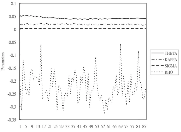
(25) volatilities are annualized. It can be seen that the MCMC volatility estimates during the 911 event (September 11, 2001) and the SARS period (around April 20, 2003 to June 3, 2003) are close to 40 percent and over 30 percent, respectively. The pattern of the path for MCMC volatility estimates is similar to that for realized volatility. Thus, the MCMC volatility estimates seem to make sense.. Figure 2: Estimated volatility paths and realized volatility for the TAIEX index 1.2 realized volatility MCMC. 1. Spot Volatility. 0.8. 0.6. 0.4. 0.2. 0 2001/1/3. 2001/5/3. 2001/9/3. 2002/1/3. 2002/5/3. 2002/9/3. 2003/1/3. 2003/5/3. 2003/9/3. Date. For the out-of-sample option pricing, the rolling procedure of the MCMC is necessary to yield estimates of the parameters involved in Heston’s model for each day between September 1, 2003 and December 31, 2003. The same process is estimated 86 times systematically using 250 past index return observations. Thus, the daily changing estimates of these parameters are. 17.

(26) used as inputs in Heston’s option-pricing formula. Figure 3 presents the evolution of the parameters associated with the stochastic variance process throughout the out-of-sample period. It should be noted that the estimates are all annualized. As we can observe from the figure, the long-term variance, θ , the rate of convergence of the instantaneous variance to the long-term average, κ , and the volatility of the variance process, σ , remain quite stable over the out-of-sample period. However, the coefficient of correlation between the shocks for the stock and the variance, ρ , changes continuously. As before, the correlation remains negative throughout the out-of-sample period.. Figure 3: MCMC estimates from September 2003 to December 2003 0.1 0.05 0. Parameters. -0.05 THETA. -0.1. KAPPA SIGMA. -0.15. RHO. -0.2 -0.25 -0.3 -0.35 1 5 9 13 17 21 25 29 33 37 41 45 49 53 57 61 65 69 73 77 81 85 Time. 18.

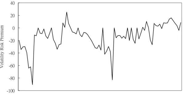
(27) 6.. Estimating the implied variance and the volatility risk premium. 6.1. Estimation procedure. Note that once we have estimated for each day the parameters of the variance process,. κ , θ , σ and ρ , and the spot volatilities, we still need to estimate the volatility risk premium, λ , before we can actually price a given call option under Heston’s model. Therefore, it seems reasonable to use cross-sectional data to implicitly infer the parameters that minimize the sum of the squared errors (SSE) in a given day of the sample. Given the set of parameters of the MCMC estimation procedure obtained for a particular. (. ). ˆ = κˆ ,θˆ , σˆ , ρˆ , and for each option, i (i = 1,…, n ) and each day day t in the sample, Ω t t t t t t , we define the pricing error as:. (. ). ˆ ,Vˆ = cˆ (K ) − c (K ) , eit λ ; Ω t t it i it i. (8). where Vˆt is the MCMC instantaneous variance estimate, cˆit (K i ) is the theoretical price of call i in day t , and cit (K i ) is the corresponding observed market price. We then want to find the risk premium parameter, λ , to solve: n. [ (. ˆ , Vˆ SSEt ≡ min ∑ eit λ ; Ω t t λ. i =1. )] . 2. (9). Figure 4 provides the daily volatility risk premium obtained by solving eq. (9). We can see that the estimated daily values of λ further suggest that the volatility risk premium varies over time in the TAIEX index option market. Notice that this time-varying behavior of the volatility risk premium is not consistent with Heston’s model since λ must be a constant value.. 19.

(28) Figure 4: Daily volatility risk premium for MCMC variance estimate 40. Volatility Risk Premium. 20 0 -20 -40 -60 -80 -100 1 4 7 10 13 16 19 22 25 28 31 34 37 40 43 46 49 52 55 58 61 64 67 70 73 76 79 82 85 Time. For out-of-sample option pricing problem, I use the previous day’s implied volatility in the BS model and compute the next day’s option price. It seems unfair to use the MCMC variance estimate of Heston’s model to compute option price. Therefore, the implied volatilities from the BS model and both the implied instantaneous variance and the volatility risk premium from the Heston model are estimated every day from option prices of our sample. Now the Eqs. (8) and (9) become. (. ). ˆ = cˆ ( K ) − c ( K ) , eit λ , Vt ; Ω t it i it i. (10). and. (. n. ). 2. ˆ ⎤ . SSEt ≡ min ∑ ⎡eit λ , Vt ; Ω t ⎦ {λ ,Vt } i =1 ⎣. (11). Direct inspection of the quadratic form in Eq. (11) shows that it is highly valley shaped and , therefore, it is extremely flat along a direction corresponding to a nontrivial combination of. λ and Vt . As a consequence, derivative-based minimization methods are expected to perform poorly since the numerically computed gradient is very unstable in the neighborhood. 20.

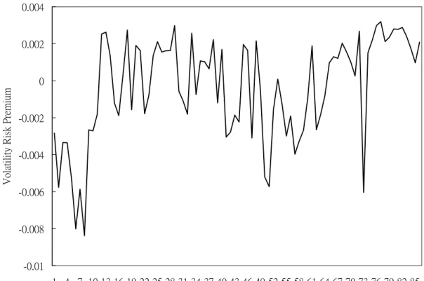
(29) of a minimum. This is confirmed by some experiments that we performed with the Newton-Raphson method. In order to avoid the above problem, a derivative-free minimization algorithm is called for. Since the function in Eq. (11) only depends on two parameters, the downhill simplex method of Nelder and Mead (1965) seems to be a natural candidate. We have checked the method by choosing randomly several starting triplets: in cases of convergence to different local minima their minimum was selected as the global solution. So we obtain daily estimates of both λ and Vt from September 1, 2003 to December 31, 2003; i.e. a sample of 86 days. Finally, a series for daily implied volatilities estimated in the corresponding BS versions of Eqs. (10) and (11) is also obtained.. 6.2. The volatility risk premium. In Figure 5, we can see that the estimated daily values of λ also vary over time, but are surprisingly close to zero. The estimated values of λ range from -0.0084 to 0.0032. The mean and median for the time-series of λ are -0.0004 and 0.0003, and the standard deviation is 0.0028. The skewness and the kurtosis are -0.8130 and 0.0315, respectively. The null hypothesis of λ = 0 was tested under two different methods. First, assuming that. λ values were drawn from a normal distribution, the Student’s t ratio was -1.3545 (p-value = 0.1792). Second, a nonparametric Wilcoxon signed-rank test for the population median of λ yielded a p-value of 0.4642. Summing up, I conclude that the evidence does not support the rejection of the null hypothesis that the volatility risk premium is zero. The finding of a zero volatility risk premium for TAIEX index options is consistent with Bakshi, Cao, and Chen (1997), who find that the maximum likelihood estimates of κ and θ are statistically indistinguishable from their respective S&P 500 option-implied counterparts, i.e., κ ∗ and. 21.

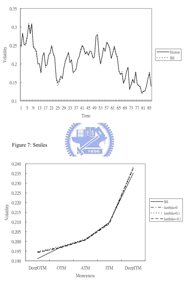
(30) θ∗.. Figure 5: Daily volatility risk premium for implied instantaneous varinace 0.004. 0.002. Volatility Risk Premium. 0. -0.002. -0.004. -0.006. -0.008. -0.01 1 4 7 10 13 16 19 22 25 28 31 34 37 40 43 46 49 52 55 58 61 64 67 70 73 76 79 82 85 Time. 6.3. Implied volatility graphs. Figure 6 contains the evolution for series of implied volatilities from September 1, 2003 to December 31, 2003 for the BS model and Heston’s model. Surprisingly, Heston’s volatility tends to be similar to BS’s volatility. To obtain a general picture of the potential misspecifications of the option-pricing models employed in this research, I report the average pattern of implied volatilities across degrees of moneyness. Since the λ parameter in Heston’s model is constant, and given that we can impose the condition λ = 0 for the volatility risk premium embedded in Heston option 22.

(31) prices on the TAIEX index according to the conclusions from the above tests, we can solve Eqs. (10) and (11) with λ = 0 and obtain a daily estimate of instantaneous variance from September 1, 2003 to December 31, 2003. I also repeat the above procedure for two alternative λ values, specifically λ = 0.1 and λ = −0.1 , in order to analyze the sensitivity of the estimated instantaneous variance under different magnitudes of λ which are in accordance with our sample of λ values. In Section 7, I will test the out-of-sample pricing performance for Heston’s model under the three candidate values of λ and compare each of them with BS’s performance. The results are shown in Figure 7. In the BS case, I obtained the implied volatility of each call option and for each day of the above period. Then the equally weighted implied volatility for each moneyness category and each day in the sample period is calculated. The pattern of the volatility curve of BS model suggests that the BS model tends to underprice deep ITM calls and overprice deep OTM calls. Any reasonable alternative model to BS must be able to properly price deep ITM and deep OTM call options. Of course, Heston’s stochastic volatility model is a potential and particularly interesting candidate. In the Heston case, and for λ = −0.1, 0.0, 0.1 , I may analyze the pattern of implied volatilities across alternative degrees of moneyness. The evidence reported in Figure 7 seems that Heston’s approach tends to underprice deep ITM calls and overprice deep OTM calls.. 23.

(32) Figure 6: Daily implied volatilities 0.35. Volatility. 0.3. 0.25 Heston BS. 0.2. 0.15. 0.1 1 5 9 13 17 21 25 29 33 37 41 45 49 53 57 61 65 69 73 77 81 85 Time. Figure 7: Smiles. 0.240 0.235 0.230. Volatility. 0.225 BS. 0.220. lambda=0. 0.215. lambda=0.1 lambda=-0.1. 0.210 0.205 0.200 0.195 0.190 DeepOTM. OTM. ATM. ITM. Moneyness. 24. DeepITM.

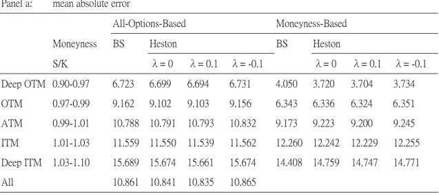
(33) 7.. Out-of-sample pricing performance. 7.1. Out-of-sample pricing error. In order to test the out-of-sample pricing performance for each model analyzed in this work, I employ 1 year of rolling data to estimate, by MCMC methods, the parameters of the stochastic variance process assumed in Eq. (1). Given these estimates and the volatility risk premium, λ , I use all call options available in the sample to compute the instantaneous variance for each day from September 1, 2003 to December 31, 2003 that minimized the sum of squared errors between the theoretical value and the market price of the call options according to Eqs. (10) and (11). I then compute the theoretical price of each option using the previous day’s instantaneous variance and the corresponding parameters of the stochastic volatility process. For the BS case, the previous day’s implied volatility that minimized the sum of squared errors between the theoretical value and the market price of the options is used to obtain the theoretical BS price of each option in the sample. In this way, I have 732 pricing errors for each of the calls available from September 2, 2003 to December 31, 2003, and for each of the models analyzed. These pricing errors are the basis for my analysis. Table 5 reports three measures of performance for the alternative model specifications. Panel A contains the mean absolute pricing error (MAE) which is the sample average of the absolute difference between the model price and the market price for each call in the testing period. Panel B reports the root mean squared error (RMSE) which is the square root of the average squared valuation error. In Panel C, the reported mean percentage pricing error (MPE) is the sample average of the theoretical price minus the market price, divided by the market price. These statistics are calculated for each moneyness category and for all calls in the sample.. 25.

(34) Pricing errors reported under the heading “All-Options-Based” are obtained using the volatility values implied by all of the previous day’s call options. And pricing errors under “Moneyness-Based” are obtained using the volatility values implied by those previous-day calls whose moneyness levels lie in the same category (OTM, ATM, or ITM) as the option being priced. Overall, Heston’s option-pricing model tends to perform slightly better than the BS model in mean absolute errors and root mean square errors. The root mean square error over all calls is approximately 14.92 NT dollars for Heston’s model independently of the volatility risk premium assumed. It is quite important to notice that the level of the volatility risk premium does not seem to have any influence on the performance of Heston’s stochastic volatility model. The pricing errors obtained under alternative λ values are practically identical. There might be some evidence in favor of a positive risk premium, but we can safely conclude that the performance of the model does not seem to be sensitive to the volatility risk premium. This is an important empirical result. Kapadia (1998) shows that the expected value of the delta-hedged gain, under a stochastic volatility model where volatility risk is not prized, is zero. This is exactly the same result that holds under the BS model. Consequently, if we may assume that volatility risk is not priced, the analysis of the dynamic hedging performance of both models is clearly facilitated. On the other hand, if volatility risk is priced, the average delta-hedged gain is proportional to the magnitude and sign of the volatility risk premium. Comparisons of the dynamic hedging performance between Heston’s model and the BS model may be much more complicated than the analysis carried out by Bakshi, Cao, and Chen (1997).. 26.

(35) Table 5: Out-of-sample pricing error Panel a:. mean absolute error. Moneyness. All-Options-Based. Moneyness-Based. BS. BS. S/K. Heston λ= 0. λ= 0.1. λ= -0.1. Heston λ= 0. λ= 0.1. λ= -0.1. Deep OTM 0.90-0.97. 6.723. 6.699. 6.694. 6.731. 4.050. 3.720. 3.704. 3.734. OTM. 0.97-0.99. 9.162. 9.102. 9.103. 9.156. 6.343. 6.336. 6.324. 6.351. ATM. 0.99-1.01. 10.788 10.791. 10.793. 10.832. 9.173. 9.223. 9.200. 9.245. ITM. 1.01-1.03. 11.559 11.550. 11.539. 11.562. 12.260. 12.242. 12.229. 12.255. Deep ITM. 1.03-1.10. 15.689 15.674. 15.661. 15.674. 14.408. 14.759. 14.747. 14.771. 10.861 10.841. 10.835. 10.865. λ= 0. λ= 0.1. λ= -0.1. All. Panel b:. root mean square error. Moneyness. All-Options-Based. Moneyness-Based. BS. BS. S/K. Heston λ= 0. λ= 0.1. λ= -0.1. Heston. Deep OTM 0.90-0.97. 10.440 10.398. 10.360. 10.451. 7.298. 6.135. 6.092. 6.173. OTM. 0.97-0.99. 13.065 13.008. 12.974. 13.076. 8.639. 8.623. 8.591. 8.657. ATM. 0.99-1.01. 14.888 14.851. 14.808. 14.921. 11.825. 11.900. 11.856. 11.940. ITM. 1.01-1.03. 15.264 15.205. 15.163. 15.253. 16.867. 16.842. 16.798. 16.888. Deep ITM. 1.03-1.10. 19.127 19.114. 19.103. 19.109. 20.224. 20.573. 20.534. 20.611. 14.962 14.928. 14.900. 14.962. All. Panel c:. mean percentage error All-Options-Based Moneyness BS. Heston. S/K. λ= 0. Moneyness-Based BS λ= 0.1. λ= -0.1. Heston λ= 0. λ= 0.1 λ= -0.1. Deep OTM 0.90-0.97. 22.798% 23.071% 23.032% 23.387% -2.531% -0.642% -0.680% -0.621%. OTM. 0.97-0.99. 9.019%. 9.392%. 9.384%. 9.447%. 1.644%. 1.730%. 1.728%. 1.728%. ATM. 0.99-1.01. 4.619%. 4.508%. 4.495%. 4.525%. 1.673%. 1.648%. 1.646%. 1.651%. ITM. 1.01-1.03. 0.018%. 0.057%. 0.052%. 0.075%. 1.217%. 1.229%. 1.224%. 1.234%. Deep ITM. 1.03-1.10. -3.054% -3.050% -3.049% -3.046% 0.181%. 0.282%. 0.280%. 0.282%. All. 7.767%. 7.889%. 7.874%. 7.995%. 27.

(36) It should be pointed out that the slightly better overall performance of Heston’s model is not maintained throughout all moneyness categories. In particular, Heston’s model tends to value ITM and OTM calls better than BS. However, the opposite results holds for ATM calls. Heston’s model, regardless of the volatility risk premium imposed, tends to overvalue OTM calls and undervalue ITM calls. In Heston’s case, the evidence points towards a sneer rather than a regular smile.. 7.2. Skewness and Kurtosis. The time-varying behavior of the correlation coefficient found above may have a serious impact on the capacity of Heston’s model to explain option-pricing data. It suggests that, in this case, we may have a problem similar to the one we have when assuming constant volatility in the BS context. If the correlation between prices and volatility changes continuously over time, skewness of the underlying asset may also exhibit time-varying behavior. This is clearly a potential and relevant problem for models with stochastic volatility. On the other hand, according to the estimates shown in Figure 3, it seems that the behavior of the volatility of variance is rather stable over time. This suggests that accounting for changing kurtosis of the underlying asset may not be as crucial as taking into consideration changing skewness. Das and Sundaram (1999) obtain closed-form expressions for conditional and unconditional skewness and kurtosis under Heston’s stochastic volatility model. Their expressions, for the frequency of ∆ = 1 , can be seen in Appendix D. Given my rolling estimates of parameters from September 2003 to December 2003, I can evaluate (C1) and (C2) in Appendix C daily, so that I may observe how the characteristics of. 28.

(37) the distribution of the underlying asset, skewness and kurtosis, change with both the correlation coefficient and the volatility of variance. Figure 8 depicts the conditional and unconditional skewness over the sample period. As we can easily observe, their behavior closely follows the pattern of the correlation coefficient of Figure 3. As expected, skewness mainly arises from the correlation between changing prices and stochastic volatility of the underlying asset. The problem is that, of course, Heston’s model assumes a constant unconditional skewness over time. In Leon and Rubio (2000), it is shown that, all else being constant, the relationship between skewness and the correlation coefficient is positive for both the conditional and unconditional cases. This explains the behavior of skewness in Figure 8. Therefore, if the correlation coefficient presents a time-varying behavior, an option-pricing model with a stochastic differential equation for correlation is a desirable extension of Heston’s model. Given this evidence, we should not expect to find a good performance of the stochastic volatility model when we compare observed market prices with theoretical prices. Figure 9 contains the same evidence for the kurtosis. In principle, the impact of time-varying kurtosis on the misspecification of Heston’s model seems to be much less severe than the influence of the correlation coefficient. Its pattern over time is much more stable than. ρ . This is related to the behavior of the volatility of variance in Figure 3. This is the parameter which will influence the kurtosis in the stochastic volatility option-pricing model, and it does not seem to change much over time. Once again, in Leon and Rubio (2000), it is shown that the relationship between kurtosis and σ is positive for both the conditional and unconditional cases. As a summary, time-varying skewness may be the key issue to analyze if we want to understand the failure of the tests we reported above. Its consequences may be much more. 29.

(38) serious than the potential effects of changing kurtosis.. Figure 8: Time-varying skewness 0.000 -0.001 -0.002. Skewness. -0.003 unconditional. -0.004. conditional. -0.005 -0.006 -0.007 -0.008 1 5 9 13 17 21 25 29 33 37 41 45 49 53 57 61 65 69 73 77 81 85 Time. Figure 9: Time-varying kurtosis 3.014 3.012 3.01 3.008 Kurtosis. 3.006. unconditional. 3.004. conditional 3.002 3 2.998 2.996 2.994 1. 6 11 16 21 26 31 36 41 46 51 56 61 66 71 76 81 86 Time. 30.

(39) 8. Conclusions. This paper introduces a two-step procedure, based on both time series and cross-section data, for estimating all the parameters that we need to compute Heston’s call price. This estimation approach should be particularly useful in thinly traded markets where a single cross-sectional estimation approach may be difficult to implement, as is the case in the Taiwan options data on the TAIEX stock index. Moreover, to employ just a cross-sectional procedure may ignore relevant information that may be included in the original series but not in the option prices. By using the MCMC methods to adjust for discretization biases, my approach combines the time-series information contained in the underlying security with the cross-sectional information embedded in option prices. On average, over all call options available in my sample, Heston’s model improves the performance of BS just marginally. It is clear that this extremely limited improvement barely justifies the implementation costs involved in the estimation of Heston’s approach.. The overall rejection of Heston’s model coincides with recent findings by Bakshi, Cao, and Chen (1997) and Chernov and Ghysels (2000) for options written on the S&P 500 index. It is also found that the daily volatility risk premium behaves in a quite volatile fashion over time. However, my evidence suggests that the implied volatility risk premium has a negligible impact on the pricing performance of Heston’s model. The findings of this paper suggest possible directions for future research. Presumably, the ultimate reasons behind the shortcomings of Heston’s model are closely related to the time-varying skewness found in the data. In particular, the assumption of a constant correlation coefficient between returns and stochastic volatility should be relaxed if we want to have a richer model. It should be clear that my results are generally applicable regardless of. 31.

(40) which market is used in the estimation. The behavioral restrictions imposed on the parameters of the diffusion process should be understood as a limitation of the stochastic volatility model. Unfortunately, of course, the complexities needed to price options seem to increase without bounds. Another potentially interesting area of research might be related to endogenously incorporating liquidity costs in option-pricing models with either stochastic volatility, stochastic jumps or both. Unfortunately, once again, this approach may be extremely demanding from a theoretical point of view.. 32.

(41) Appendix A. Heston’s stochastic volatility option pricing formula. The Heston’s option pricing formula is given by: c ( S , v, t ) = St P1 − e. − r (T − t ). KP2 ,. where S t is the underlying spot price, K is the exercise price and the probabilities are given by: Pj =. 1 1 + 2 π. ∫. ∞. 0. ⎡ e − iφ ln [K ] f j ⎤ Re ⎢ ⎥ dφ , j = 1, 2 , iφ ⎢⎣ ⎥⎦. where Re( y ) is the real part of the function y ; i is the imaginary number i = − 1 , and f j ( x, v, T − t ; φ ) = exp[C (T − t ; φ ) + D (T − t ; φ )v + iφx ] ,. where, C (T − t ; φ ) = rφi (T − t ) +. ⎡1 − ge d (T −t ) ⎤ ⎫ a ⎧ ( ) ( ) − + − − b i d T t 2 ln ρσφ ⎨ j ⎢ ⎥⎬ , − 1 g σ2 ⎩ ⎣ ⎦⎭. b j − ρσφi + d ⎡ 1 − e d (T −t ) ⎤ D(T − t ;φ ) = , ⎢ d (T − t ) ⎥ σ2 ⎣1 − ge ⎦ g= d=. b j − ρσφi + d b j − ρσφi − d. (ρσφi − b ). 2. j. ,. (. ). − σ 2 2u j φi − φ 2 ,. a = κθ , b1 = κ + λ − ρσ , b2 = κ + λ , u1 = 1 2 , u 2 = −1 2 , verifying that C (0) = D(0) = 0 , and C (T − t ; φ ) and D(T − t; φ ) ( and therefore the probabilities Pj ; j = 1,2 ) depend on the vector of the parameters, (κ ,θ , λ , σ , ρ ) given by the processes assumed by Heston under the original probability. 33.

(42) Appendix B. Posterior Distributions for Volatility. The conditional posteriors for the parameters are standard. Given the conjugate priors, the conditional posteriors for. {µ , κ , θ , σ }. are all standard distributions, and I omit the. derivations as they can be found in standard texts. For ρ I use an independence Metropolis algorithm with a proposal density centered at the sample correlation between the Brownian. (. ). increments. The conditional posterior for volatility, p Vt∆ | Yt∆ , V( t +1)∆ , V( t −1)∆ , Θ , is not a known distribution. To sample from it, I use a random-walk Metropolis algorithm (see Johannes and Polson (2003)). I now discuss the choices of prior distributions and parameters. Wherever possible, I choose standard conjugate priors, which allows me to directly draw from the conditional posteriors. My prior distributions for the parameters are: µ ~ N (0, 25) , κθ ~ N (0,1) ,. κ ~ N (0,1) , σ 2 ~ IG (2.5, 0.1) , and ρ ~ U (− 1, 1) , where IG refers to the Inverse Gamma distribution, and U a standard uniform distribution. All of the prior distributions are close to noninformative.. 34.

(43) Appendix C. (Un)conditional skewness and kurtosis. The conditional case: ⎡ κ κ κ ⎤ ⎛ 3σρ eκ 2 ⎞ ⎢θ ( 2 − 2e + κ + κ e ) − v (1 + κ − e ) ⎥ , SKEW = ⎜ ⎟ 32 ⎥ κ ⎠ ⎢ ⎡θ (1 − eκ + κ eκ ) + v ( eκ − 1) ⎤ ⎝ ⎢⎣ ⎣ ⎥⎦ ⎦. ⎡ ⎛ θ A − vA2 ⎞ ⎤ KURT = 3 ⎢1 + σ 2 ⎜ 1 ⎟⎥ , B ⎝ ⎠⎦ ⎣. (C1). where A1 = (1 + 4eκ − 5e 2κ + 4κ eκ + 2κ e 2κ ) + 4 ρ 2 ( 6eκ − 6e 2κ + 4κ eκ + 2κ e 2κ + κ 2 eκ ) A2 = 2 (1 − e 2κ + 2κ eκ ) + 8 ρ 2 ( 2eκ − 2e 2κ + 2κ eκ + κ 2 eκ ) B = 2κ ⎡⎣θ (1 − eκ + κ eκ ) + v ( eκ − 1) ⎤⎦ , 2. and where v ≡ Vt .. The unconditional case:. ⎛ σρ ⎞ ⎡1 − eκ + κ eκ ⎤ SKEW = 3 ⎜ ⎥, ⎟⎢ 32 κ ⎝ κθ ⎠ ⎣ κ e ⎦ ⎡ ⎤ σ2 KURT = 3 ⎢1 + 1 − eκ + κ eκ + 4 ρ 2 ⎡⎣ 2 − 2eκ + κ + κ eκ ⎤⎦ ⎥ . 2 κ ⎣ κθκ e ⎦. (. ). 35. (C2).

(44) References. Aït-Sahalia, Yacine, 1996a, Testing continuous-time models of the spot interest rate, Review of Financial Studies 9, 385-426. Aït-Sahalia, Yacine, 1996b, Nonparametric pricing of interest rate derivative securities, Econometrica 64, 527-342. Andersen, Torben, L. Benzoni, and J. Lund, 2002, Towards an empirical foundation for continuous-time equti return models, Journal of Finance 57, 1239-1284. Andersen, Torben, H. Chung, and B. Sorensen, 1999, Efficient method of moments estimation of a stochastic volatility model: A Monte Carlo study, Journal of Econometrics 91, 61-87. Bakshi, G., C. Cao, and Z. Chen, 1997, Empirical performance of alternative option pricing models, Journal of Finance 52, 2003-2049. Bates, David, 1996, Jumps and stochastic volatility: Exchange rate processes implicit in Deutche mark options, Review of Financial Studies 9, 69-107. Black, Fischer, and Myron Scholes, 1973, The pricing of options and corporate liabilities, Journal of Political Economy 81, 637-654. Bollerslev, T., 1986, Generalized Autoregressive Conditional Heteroskedasticity, Journal of Econometrics 31, 307-327. Chernov, Mikhail, and E. Ghysels, 2000, Towards a unified approach to the joint estimation of objective and risk neutral measures for the purpose of options valuation, Journal of Financial Economics 56, 407-458.. 36.

(45) Das, S., and R. Sundaram, 1999, Of smiles and smirks: a term-structure perspective, Journal of Financial and Quantitative Analysis 34, 211-239. Duffie, D., and P. Glynn, 1997, Estimation of continuous-time Markov processes sampled at random time intervals, Mimeo, Stanford University. Duffie, D., and K. Singleton, 1993, Simulated moments estimation of Markov models of asset prices, Econometrica 61, 929-952. Engle, R.F., 1982, Autoregressive Conditional Heteroskedasticity with Estimates of the Variance of U.K. Inflation, Econometrica 50, 987-1008. Eraker, B., 2001, MCMC analysis of diffusion models with application to finance, Journal of Business and Economic Statistics 19-2, 177-191. Eraker, B., 2003, Do equity prices and volatility jump? Reconciling evidence from spot and option prices, Working paper, Duke University. Eraker, B., M. Johannes, and N. Polson, 2003, The impact of Jumps in equity index volatility and returns, Journal of Finance 58, 1269-1300. Fiorentini, G., A. León, and G. Rubio, 2002, Estimation and empirical performance of Heston’s stochastic volatility model: the case of a thinly traded market, Journal of Empirical Finance 9, 225-255. Gallant, A. Ronald, and George Tauchen, 1996, Which moments to match, Econometric Theory 12, 657-681. Gouriéroux, C., A. Monfort, and E. Renault, 1993, Indirect inference, Journal of Applied Econometrics 8, S85-S118. Hansen, L. P., and J. A. Scheinkman, 1995, Back to the future: generating moment implications for continuous time Markov processes, Econometrica 63, 767-804. Heston, S., 1993, A closed-form solution for options with stochastic volatility with. 37.

(46) applications to bond and currency options, Review of Financial Studies 6, 327-344. Heston, S., and S. Nandi, 2000, A closed-form GARCH option valuation model, Review of Financial Studies 13, 585-625. Hull, J., and A. White, 1987, The pricing of options on assets with stochastic volatilities, Journal of Finance 42, 281-300. Jacquier, Eric, N. Polson, and P. Rossi, 1994, Byesian analysis of stochastic volatility models, Journal of Economics and Business Statistics 12, 371-389. Johannes, Michael, and N. Polson, 2002, MCMC methods for continuous-time financial econometrics, in Yacine Ait-Sahalia and Lars Hansen, eds.: Handbook of Financial Econometrics (Elsevier, New York). Jones, Christopher, 1998, Bayesian estimation of continuous-time finance models, Working paper, Simon School of Business, University of Rochester. Kapadia, N., 1998, Do equity options price volatility risk? Empirical evidence, Working Paper, University of Massachusetts. Kessler, M., and M. Sorensen, 1999, Estimating equations based on eigenfunctions for a discretely observed diffusion, Bernoulli 5, 299-314. Leon, A., and G. Rubio, 2000, Smiling under stochastic volatility, unpublished manuscript, University of Alicante and University of Pais Vasco. Melino, A., 1994, Estimation of continuous-time models in finance, in Advances in Econometrics, Sixth World Congress, Volume II, ed. by C. Sims, Cambridge, UK: Cambridge University Press. Merton, Robert C., 1973, Theory of rational option pricing, Bell Journal of Economics 4, 141-183. Merton, Robert C., 1980, On estimating the expected return on the market: an exploratory. 38.

(47) investigation, Journal of Financial Economics 8, 323-361. Nelder, J.A., and R. Mead, 1965, A simplex method for function minimization, Computer Journal 7, 308-313. Pan, Jun, 2002, The jump-risk premia implicit in options: Evidence from an integrated time-series study, Journal of Financial Economics 63, 3-50. Robert, Christian, and George Casella, 1999, Monte Carlo Statistical Methods (Spreinger-Verlag). Scott, L.O., 1987, Option pricing when the variance changes randomly: theory, estimation and an application, Journal of Financial and Quantitative Analysis 22, 419-438. Stanton, R., 1997, A nonparametric model of term structure dynamics and the market price of interest rate risk, Journal of Fiance 52, 1973-2002. Sundaresan, Suresh M., 2000, Continuous-time methods in finance: A review and a assessment, Journal of Finance 55, 1569-1622. Wiggins, J.B., 1987, Option values under stochastic volatilities: theory and empirical estimates, Journal of Financial Economics 19, 351-372.. 39.

(48)