蛋白質結構與動態之關係

國

立

交

通

大

學

生物資訊研究所

碩

士

論

文

蛋白質結構與動態之關係

On the relationship between protein structure and dynamics

研 究 生：張瓊文

指導教授：黃鎮剛 教授

蛋白質結構與動態之關係

On the relationship between protein structure and dynamics

研 究 生：張瓊文 Student：Chiung-Wen Chang

指導教授：黃鎮剛 Advisor：Jenn-Kang Hwang

國 立 交 通 大 學

生物資訊研究所

碩 士 論 文

Submitted to Department of Computer and Information Science College of Electrical Engineering and Computer Science

National Chiao Tung University in partial Fulfillment of the Requirements

for the Degree of Master

in Bioinformatics

July 2008

Hsinchu, Taiwan, Republic of China

蛋白質結構與動態之關係

學生：張瓊文

指導教授：黃鎮剛

國立交通大學生物資訊研究所碩士班

摘 要

蛋白質的功能與動態相關。由於結構生物學的進步，存放於蛋白質資料

庫 (the Protein Data Bank, PDB) 的蛋白質結構數目快速增加，如何由結構

資訊有效率地導出蛋白質動態相當重要。最近的研究中，質量中心模型

(Centroid model, CM) 與加權接觸數模型 (Weighted contact number model,

WCN)皆成功利用結構資訊重現溫度因子 (temperature factor or B-factor)。在

本篇論文中，我們發現另外一個重要的結構特徵: 溶劑可接觸表面 (Solvent

accessible surface, SAS)與溫度因子相關。此外，使溶劑可接觸表面設定檔

(profile)平滑，與溫度因子間的關聯係數可更增進。我們用數據化統計方式

研究這些特徵/模型，結果顯示它們彼此為高度相關。雖然根本的物理原理

尚不明瞭，然而這些發現幫助我們更加了解蛋白質結構與動態的關係。

On the relationship between protein structure and dynamics

Student: Chiung-Wen Chang

Advisor: Jenn-Kang Hwang

Institute of Bioinformatics

National Chiao Tung University

ABSTRACT

With the progress in experimental structural biology, the number of protein

structures deposited in Protein Data Bank (PDB) grows rapidly. Hence, it is

important to extract dynamic properties from protein structures efficiently. In

recent researches, the Centroid model (CM) and the Weighted contact number

model (WCN) were successful in reproducing B-factor from structural

information. In this study, we discovered that another important structural

feature: solvent accessible surface (SAS) is related to B-factor. Moreover,

smoothing SAS profile can further improve its correlation with B-factor. We

performed numerical statistical analysis on these features/models and the results

showed that they are highly correlated with one another. Although the

underlying physical principles remain unclear, our results will be useful in the

study of protein structure-dynamics relationship.

誌謝辭 聽說有人誌謝辭寫到兩頁，於是我也要來挑戰。 首先要感謝我的父母家人，在我成長及求學過程中對我的付出與包容，我實在不能 算是個乖小孩，相信令他們十分頭痛。 此外最感謝的就是指導教授黃鎮剛老師，可惜因為我個人時不時會懶病發作，外加 到碩二上都一直待在球隊，沒有全心全意專注在研究上，直到最近才稍微對自己所在的 領域有皮毛的了解。我由衷感佩教授不吝提供學生在研究方面所需的一切器材，讓學生 們能放心鑽研學問，這樣的慷慨大方並不是每個教授都能夠做得到的。 謝謝草霸陸志豪學長，帶我進入這個實驗室，認識一同在博愛打球的朋友們，了解 到有人的好球帶會跟一般正常人差很多，要把球做到裁判椅的位置或樹上他才能用力打 下去。隨著一起打球的朋友們陸續離開學校，再共聚打球的機會難求，希望大家一切順 利。 謝謝偶而被我們凹時會大方出錢、堂堂助理教授卻常常跑來跟我們一起打電動的林 勇欣學長，可惜我跟你年紀差太多，很難介紹女生跟你認識。感謝尤禎祥學長、聽說記 得O’Reilly 動物與書名對應的奇妙學長施建華、字很好看四個主星在雙魚根本應該當女 生的黃存操學長辛苦地保養與管理機器，雖然後兩者跟我介紹的女生都沒有擦出火花， 我真的很遺憾，有認識好女生的話我會繼續努力。 謝謝黃少偉學長及游景盛學長對我研究上的指導，祝福林志鵬學長與徐蔚倫學姐感 情順利，連師母都有在關注你們的發展。謝謝幾乎顏士中學長與賴彥龍學長，看你們互 槓是研究生活的樂趣之一。謝謝李啟文學長與林肇基學長，他們的態度有值得我學習的 地方，及梁涵堃學長，對增進我人際方面應對進退的功力有正向作用。啊…還有時常被 發現在偷笑或被忽略的陳志杰學長，我絕對沒有又差點把學長dororo 化，每次看到學長 總是認真的在做研究，相當令人敬佩。 接下來是同屆的強者我同學松煩，更正，是于松桓同學，會寫錯肯定真的保證百分 之一百不是因為老闆一直念錯，他對研究、小遊戲與NBA 都有異於常人的偏執，在學 習方面的態度我望塵莫及。另外是何仙蕾同學，她模糊焦點的能力非常人得以望其項

背，樂天的精神十分令我欽佩。 感謝器宇非凡是慧根的學妹官慧根，再次更正，是官慧雯，必須更正也肯定真的保 證百分之一百不是因為怕她會打我或罵我賤拔辣。我們之間互相幫助，激勵對方成長， 我沒有要宣傳卡內基的意思，總之不論是研究、美食、合購乃至於電動方面的切磋，都 讓我們在各方面得到進步，祝福她及她男人衛先生得到幸福。另外還有學弟妹林子琳及 劉人維，以及在我碩士生活最後幾個月才加入實驗室的新助理簡曉芬，雖然有時跟她講 話很傷腦細胞，但她還是積極地融入我們實驗室，幫忙處理許多雜事與忍受小胖的囉 嗦，讓我們做研究能無後顧之憂，辛苦了。 對於CD-W 在改善實驗室氣氛、促進實驗室的團結(或分裂？)方面的貢獻，我特別 提出來表揚。“照顧後進！多少飯局假汝之名而行＂，八卦始終來自於人性，誠不欺也。 最後特別要謝謝張忠翔先生，張朝坤先生與張女士，雖然因為你們，存操學長跟慧 雯學妹時常猜測在他們畢業前是否能吃到我的喜酒，還是要謝謝你們以開朗的態度支持 我度過碩二下這段時間，讓我能用更正面的態度來面對我在學業上遭遇到的挑戰。

CONTENTS

摘 要...i

ABSTRACT ...ii

CONTENTS ... v

TABLE CONTENTS ...vi

FIGURE CONTENTS...vii

1. INTRODUCTION ... 1

2. MATERIALS AND METHODS ... 3

2.1 Dataset ... 3

2.2 Features and models ... 3

2.2.1 B-factor ... 3

2.2.2 Centroid model... 3

2.2.3 Weighted contact number (WCN) model... 4

2.2.4 Gaussian network model (GNM)... 4

2.2.5 Solvent accessible surface (SAS) ... 5

2.3 Methods ... 5

2.3.1 The relationship between protein structure and dynamics ... 5

2.3.2 The relationship between B-factor and smoothed SAS... 6

2.3.3 The effect of SCOP classification and protein length... 7

3. RESULT AND DISCUSSION... 8

3.1 The relationship between protein structure and dynamics ... 8

3.2 The relationship between B-factor and smoothed SAS/PSAS ... 9

3.3 The effect of SCOP classification and protein length ... 10

4. CONCLUSION ... 11 REFERENCES ... 13 TABLE CAPTIONS ... 15 TABLES... 16 FIGURE CAPTIONS ... 23 FIGURES ... 24 APPENDIXES... 32

TABLE CONTENTS

Table 1. Maximum accessible surface area of amino acids ... 16

Table 2. Criteria used in

PDB-REPRDB for the dataset

Table 3. Descriptions of SCOPa classes...18

Table 4. The range and the number of proteins of each group... 19

Table 5. The average correlation coefficients for the dataset... 20

Table 6. The average correaltion coefficient between B-factor and smoothed SAS profiles .. 21

FIGURE CONTENTS

Figure 1. Comparison of B-factor and SAS, WCN, GNM and smotthed SAS profiles ... 24

Figure 2. SAS profile, B-factor putty/surface of 1A1IA and smoothed SAS profile ... 26

Figure 3. The histogram of the distribution of protein length in the dataset ... 28

Figure 4. Mean B-factor, CM, SAS and WCN distribution of each length group... 29

1. INTRODUCTION

Protein dynamics is closely related to protein function. For instance, catalytic residues are found to be associated with high force constants and thus can be applied in catalytic residue prediction1. The ability to compute dynamic properties of proteins may help shed new light on protein function. On the other hand, protein structure may also be useful information for function prediction. Several methods have been developed for detecting pocket regions as potential active sites of enzymes2; 3.

With the progress in experimental structural biology, the number of protein structures deposited in Protein Data Bank (PDB)4 grows rapidly. More specifically, the number of protein structures deposited in PDB4 has nearly quadrupled since 2000. Hence, it becomes increasingly important to develop more efficient methods to extract dynamic properties from protein structures in a high throughput manner.

One of the important features of protein structure is solvent accessible surface (SAS). SAS is an important structural characteristic because molecular interaction occurs on the surface. It reflects the degree to which a residue interacts with the solvent molecules. SAS also suggest the folding state of a protein. Accurate prediction of solvent accessible surface can aid the prediction of other structural properties such as protein secondary structure.

The dynamic properties of proteins result from a network of complex interactions like covalent bonding and nonbonded electrostatic or van der Waals interactions. In X-ray structures, the B-factor (or temperature factor) describes the magnitude of atomic mean-square displacement. The larger the value, the greater the atom fluctuates. To compute dynamic properties of proteins, one usually resorts to molecular dynamics simulations5; 6; 7; 8; 9, which involves integrating long time trajectories of protein structure using empirical force field. Though molecular dynamics is a powerful method, it is computationally expensive. Thus Elastic network model (ENM) or Gaussian network model (GNM)10; 11; 12, have gained more popularity since they require no trajectory integration and can be applied on larger

proteins.

Although GNM seems appealing, some later developments, the Centroid model (CM)13 and the weighted contact number (WCN) model, managed to reproduce dynamic properties with simpler and more efficient way. The former discovered that atomic fluctuation is linearly related to the square of the atomic distance from the center of mass of the protein. The latter showed that B-factor profiles can be directly derived from protein contact number with weight being the square of the reciprocal distance between the contacting pair.

But the extent to which protein structures are related to dynamic properties remains unclear. To further investigate structure-dynamics relationship, we studied the relationship between SAS and B-factor in the same dataset and criteria used by other investigators14; 15. CM, WCN and GNM were also included in the analysis for the completeness of the study. We performed a statistical analysis on B-factor/CM/WCN/GNM/SAS.

The correlation coefficient between SAS and B-factor showed that these two features are correlated with each other. After the comparison with other profiles, we have noticed that the ruggedness of SAS profile might weaken its correlation with B-factor. This observation gave rise to the idea of smoothing SAS profiles.

To proof this postulation, we performed different types of smoothing processes on SAS profiles. Moreover, the same smoothing processes were also executed on SAS prediction profiles. The result showed that smoothing processes as naïve and simple as taking average with neighboring residues help improve the correlation with B-factor.

For the integrity, we also investigated the effect of protein length on the features/models and their mutual correlation. Finally, we analyzed how SCOP classification influences the mutual correlation of features/models studied here.

There are roughly three stages in our study:

(I) The correlation coefficient among B-factor, Centroid model(CM)13, Gaussian network model (GNM)10, solvent accessible surface(SAS) and Weighted contact number(WCN)14.

(II) The relationship between smoothed SAS and B-factor. (III) The effect of protein length and SCOP16 classification.

We believe that the result of our analysis will be useful in the study of protein structure-dynamics relationship.

2. MATERIALS AND METHODS

2.1 Dataset

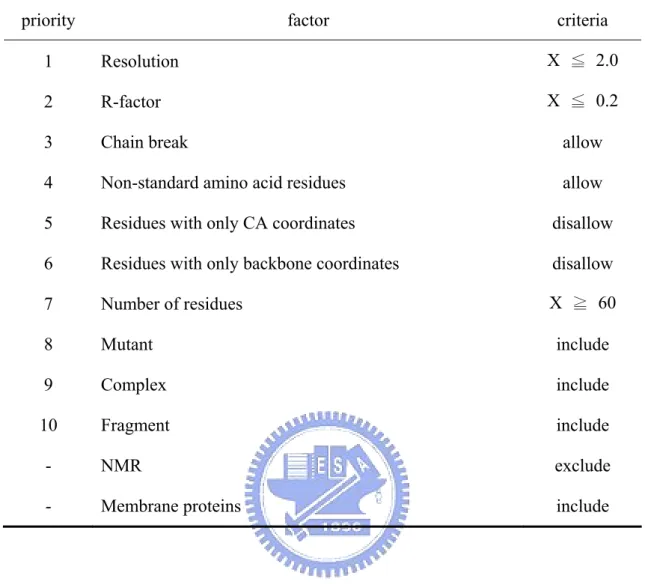
The dataset used in the present study consists of 972 protein chains from PDB-REPRDB17. According to the same criteria used in the research of WCN14, we chose X-ray crystallographic structures with resolution under 2.0Å and R-factor less than 0.2. All chains have at least 60 residues, and share pair-wise identity less than 25%. Detailed criteria can be found in Table 2.

2.2 Features and models

2.2.1 B-factor

X-ray diffraction data provide the average structure of a protein in a crystal as well as the scale of its atomic fluctuations normally expressed as the isotropic Debye-Waller factors, or B-factors. We retrieved the B-factor from PDB records.

2.2.2 Centroid model

With structural information, CM13 managed to reproduce protein dynamics and correlation of the fluctuations in proteins. It simply calculates the square of the atomic distance from the center of the mass of the protein. Let X0 be the center of mass of the protein, i.e.

∑

∑

=

k k km Xk k m

X₀ , where mk and Xk are the mass and the crystallographic position of

atom k, respectively. The distance between atom i and the center of mass can be obtained by:

) )( ( _{0 0} 2 X X X X − − = i i i r (1)

This value is found to be linearly related to the average atomic fluctuation in proteins.

Unlike Molecular dynamics (MD)5; 6; 7; 8; 9 or Elastic network model (ENM) which based on mechanical model, either sophisticated or simplified, CM depends only on the information of protein geometrical shape. CM involves no computation of proteins’ trajectories or matrix operation and thus is simple and efficient.

2.2.3 Weighted contact number (WCN) model

A recent study19 showed that the atomic mean-square displacement (or B-factor) is closely related to the number of neighboring atoms. This method was referred to as the protein contact number (CN) model. The CN model was able to predict B-factor profiles directly from protein structures without either trajectory integration or matrix diagonalization. However, the CN model can be further improved by introducing a weight being the square of reciprocal distance between the contact pair.

The weighted contact number vi of residue i is given by

∑

The WCN profile of a protein of N residues is defined as: )

,..., ,

( _{1 2} N

w= ω ω ω (3)

where ωi is defined as the inverse value of vi.

2.2.4 Gaussian network model (GNM)

The Gaussian Network Model (GNM)10 simplifies a protein by modeling it with its Cα atoms only and attaching springs with uniform constants to contacted Cα pairs. Cα pairs are

considered to be in contact when their separation distance is within a cutoff distance rc ,

typically set to 7.0±0.5Å. In GNM, all the dynamic properties can be obtained from the Kirchhoff matrix T whose elements are given by:

if i≠j and Rij r≦ c

if i≠j and Rij > rc (4)

if i=j

where Rij is the distance between atom i and j, and rc is the cutoff distance. The mean square

fluctuations of each atom and the theoretical B-factors can be expressed as:

[ ]

2.2.5 Solvent accessible surface (SAS)

The surface area is an important structural characteristic because interaction with other molecules happens on the surface. The solvent accessible surfaces of residues were assigned by using the program DSSP18. The data listed in column “ACC” of each residue was retrieved and divided by the maximum area of that amino acid. The maximum accessible area of each amino acid is listed in Table 1. The relative SAS were listed in the order of residue number to obtain SAS profiles for each protein.

2.3 Methods

2.3.1 The relationship between protein structure and dynamics

For the convenience of comparison between features with quite different ranges, we first calculated the z-scores of the values in five feature/model profiles. Z-scores is also called

⎪ ⎪ ⎨ = Γ_ij 　0 ⎩ i,i≠ j ij ⎪ Γ −

∑

standard score, z-value, normal score and standardized score. It indicates how many standard deviations an observation is above or below the mean. The z-score of the ith(i=residue number) value in the profile X is defined as:

σ μ − = i i X X z( ) (7)

, where μ is the mean and σ is the standard deviation of the distribution of values in profile X. The calculations are described by the following formulas:

X X N N i i = =

∑

∑

After z-score normalization, we calculated the correlation coefficient (CC) of two feature/model profiles X and Y by:

2 2 2 2 ₍

∑

∑

∑

∑

∑

∑

∑

If X and Y are independent then the correlation is 0. The closer the coefficient is to either −1 or 1, the stronger the correlation between the variables.

2.3.2 The relationship between B-factor and smoothed SAS

To understand how smoothing would influence the correlation coefficient between SAS and B-factor, different smoothing processes were performed on SAS profiles and predicted SAS profiles.

SAS prediction is accomplished by running the Protein Solvent AcceSsibility Prediction Server (http://140.113.239.214/~weilun/) developed by Shu WL and Hwang JK. We used the FASTA sequences of all 972 chains in our dataset as the input and chose the real-value model of this server. As a result, predicted SAS profiles (PSAS profile) could be obtained.

implemented. The basic idea of both methods is the same. They simply took the average SAS of residue i along with its neighboring (in sequence order) residues within a certain window size. The smoothed SAS (SASi’) of residue i can be calculated by:

(1) WSn(window-size n, where n=2k+1, k=1,2,3,4) n SAS SAS k i k i j j i

∑

k k j j k i k i j j i j i SAS SAS 2 2 2 ' 0 1₋ =

∑

∑

The only difference between the two types of methods is that, in modified version, each value is multiplied with a weight before calculating the average. The weight reduces as the distance from the center of the current window (residue i) increases. Take mWDW5 as an example, SASi’=(SASi-2 +2*SASi-1 +22* SASi +2* SASi+1 + SASi+2)/(1+2+22+2+1).

2.3.3 The effect of SCOP classification and protein length

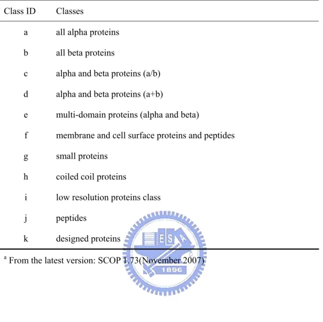
The dataset was classified into 11 groups according to SCOP database16. The following two cases were not assigned to any class and were ignored in this part of analysis: (1) chains with no SCOP entries (noted as N/A in this work) and (2) chains that are separated into segments being assigned to different classes (noted as M).

The notation and description of each class can be found in Table 3. The PDBID assigned to each class were listed in Appendix 1. The averages of ten types of correlation coefficient were also calculated on the basis of SCOP grouping.

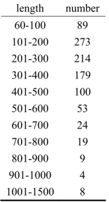
On the other hand, our dataset was divided into 11 groups according to protein length. The range and number of each group were listed in Table 4. The members’ PDBID were listed in Appendix 2.

To understand the influence of protein length, we first consider one feature/model at a time. For a protein with size N, the mean B-factor was computed by:

N B B N i i

∑

Mean CM/SAS/WCN was derived in the same way for each protein. These values were also classified according to protein length.

The result in part 1 was ten types of correlation coefficients (CCB-CM, CCB-GNM, CCB-SAS,

CCB-WCN, CCCM-GNM, CCCM-SAS, CCCM-WCN, CCGNM-SAS, CCGNM-WCN, CCSAS-WCN) for 972

proteins. For each type of correlation coefficient, we calculated the average of each group. As a result, each type of correlation coefficient would yield 11 values. Each value represents the general condition of proteins with length in the same range.

3. RESULT AND DISCUSSION

3.1 The relationship between protein structure and dynamics

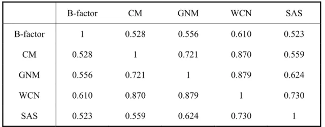
Ten types of correlation coefficients (CCB-CM, CCB-GNM, CCB-SAS, CCB-WCN, CCCM-GNM,

CCCM-SAS, CCCM-WCN, CCGNM-SAS, CCGNM-WCN, CCSAS-WCN) were calculated. The average

correlation coefficients over 972 proteins were listed in Table 5.

The lowest value was the correlation coefficient between B-factor and SAS (CCB-SAS),

0.523. However, it still shows that these two features are positively correlated to each other. In other words, the more a residue is exposed, the greater it fluctuates.

The highest value was CCGNM-WCN (0.879). Note that the inverse of original weighted

contact number was taken when building WCN profile. If a residue is located in a more crowded region, it yields a lower value in the WCN profile. From the fairly high value of

CCGNM-WCN, one can presume that this residue would exhibit higher autocorrelation of atomic

Comparing the three models built for interpreting dynamic properties from structural information: CM, GNM and WCN, WCN outperformed the others in this dataset. (CCB-CM=0.528, CCB-GNM=0.556, CCB-WCN=0.61)

Although CM, GNM and WCN are based on different theoretical hypothesis, they shared high mutual correlation with one another (CCCM-GNM=0.72, CCCM-WCN=0.870 and

CCGNM-WCN=0.879). A possible reason is that, the underlying physical property of protein can

be expressed in different way. There might be some interchangeability among these three models.

B-factor, CM and GNM depict protein dynamic properties, while SAS and WCN represent structural characteristics. Nevertheless all the five features were highly positively correlated with one another (with mutual correlation 0.523-0.879). This is in accordance with our basic concept that protein structure is related to dynamics.

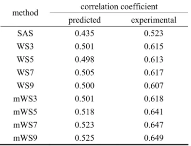
3.2 The relationship between B-factor and smoothed SAS/PSAS

As we mentioned earlier, CCB-SAS posses the lowest value (0.523) among the ten types of

correlation coefficients. Comparing the profile of B-factor, SAS, GNM and WCN (see Figure 1.(A) to (C)), SAS profile is especially rough than the others. However, if we took the average value of SAS with adjacent residues as the new SAS, the correlation with B-factor can be fairly improved (see Figure 1.(D)). These observations gave rise to the idea of smoothing SAS.

Picture that a protein segment {residuei-1, residuei, residuei+1} is exposed to the surface.

However, residuei is bended or hustled toward the center during folding. Under such

circumstances, it’s likely that some parts of the accessible surface of residuei be considered

closer to residuei-1 and residuei+1. Consequently, sharp peaks are seen throughout the plot of

SAS. Although residuei is also close to the surface and might exhibit high flexibility, it’s hard

Take 1A1IA as an example, the plot of SAS in residue-number ordering is in Figure 2(A). The z-score of b-factor was 2.684, 2.149 and 2.656 for SER-111, CYS-112 and ASP-113, respectively. 1A1IA in B-factor putty was drawn in Figure 2(B). The proportional SAS of CYS-112 was 0.134, while SER-111 was 0.806 and ASP-113 was 0.878. In terms of z-score, CYS-112 was -1.375, while SER-111 was 1.553 and ASP-113 was 1.863. The surface of 1A1IA can be found in Figure 2(C). The surface area belonged to CYS-112 was colored red. As a whole, SER-111, CYS-112 and ASP-113 bear similar B-factor but the SAS of CYS-112 is much smaller than the other two.

Here rises the need of smoothing SAS. Taking the average of the SAS within a certain window size helps us learn more about how a residue is exposed or buried.

The average CCB-SAS’ and CCB-PSAS’ derived from eight different types of smoothing

processes along with CCB-SAS and CCB-PSAS can be found in Table 6.

Smoothing either experimental or predicted SAS show meaningful improvement in the correlation with B-factor. For predicted SAS (CCB-PSAS=0.435), smoothing could uplift the

correlation to 0.525, which is comparable to experimental CCB-SAS (0.523). Greater

performances could be observed in experimental SAS. All eight smoothing processes help gain 0.08-0.12 of improvements than CCB-SAS (0.523).

The result of these simple and intuitive smoothing processes indeed support our postulate: Smoothing SAS related better to B-factors.

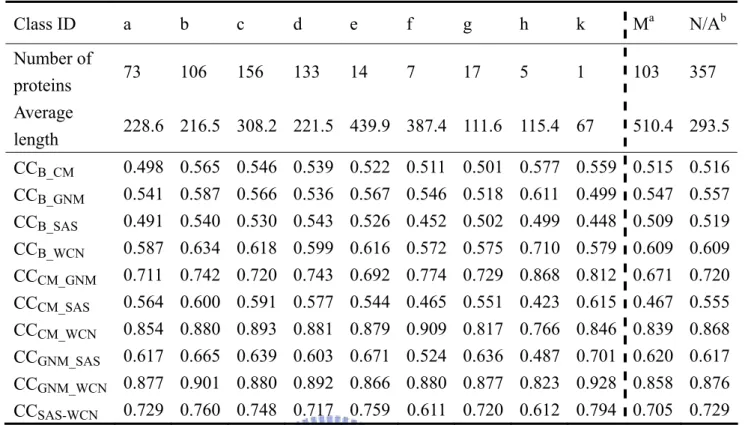
3.3 The effect of SCOP classification and protein length

The result of SCOP classification is shown in Table 7. There might be some messages lie in

the data. For example, coiled coil proteins not only possess highest CCB-CM, CCB-GNM,

CCB-WCN, CCCM-GNM, but also lowest CCCM-SAS, CCCM-WCN, CCGNM-SAS, CCGNM-WCN among all

classes. On the other hand, designed protein possesses lowest CCB-GNM, CCB-SAS and highest

protein and designed protein in our dataset are too small to be statistically meaningful (5 and 1, respectively). Studying the characteristics of each type (SCOP class) of structures would help us understand the underlying correlation. However, over 1/3 of proteins in the dataset (357/972) are lack of SCOP entries. Such circumstances left uncertainties in the final result. The effect of structural classification can be further investigated as SCOP entries become more completed.

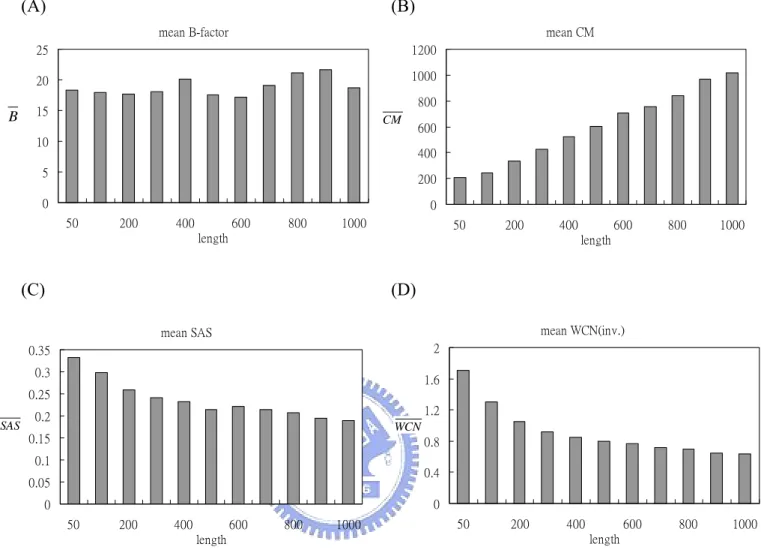
The distribution of each period of length is shown in Figure 2. The average length of the dataset is 294.16.

In Figure 4. (A)-(D) showed the average mean B-factor/CM/SAS/WCN. Unlike CM/SAS/WCN, the curve of B-factor shows neither linear nor exponential relationship with protein length. From Figure 4. (B) one can tell that in larger proteins each residue is more distant from protein centroid on average. On the contrary, residues in smaller protein expose more to the surface area. Figure4. (D) gave us a hint that residues tend to be more packed with each other when protein grows larger.

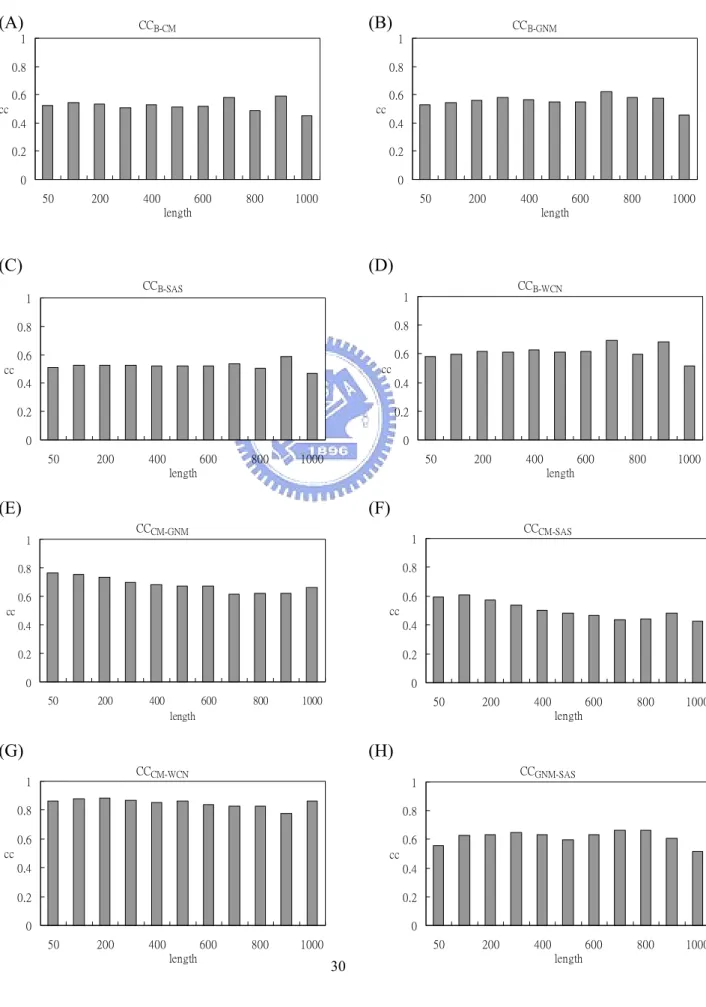
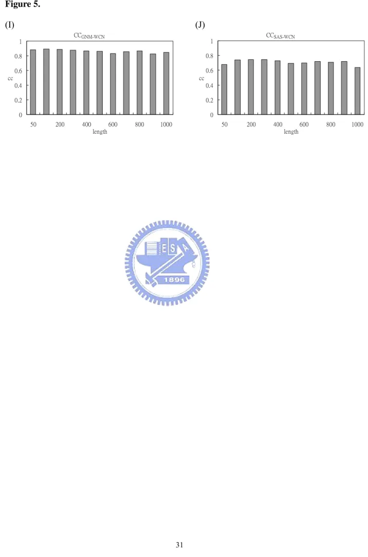
The average correlation coefficients (CCB-CM, CCB-GNM, CCB-SAS, CCB-WCN, CCCM-GNM,

CCCM-SAS, CCCM-WCN, CCGNM-SAS, CCGNM-WCN, CCSAS-WCN) of each length period were

displayed in Figure 5.(A)-(J). No obvious trends were found.

4. CONCLUSION

In order to understand protein structure-dynamics relationship, we performed a numerical statistical analysis on a dataset comprising 972 chains. We calculated the correlation coefficients among B-factor/CM/GNM/SAS/WCN. The results have shown that all the five features/models are highly positively correlated with one another. Comparing the correlation coefficients between B-factor and other features/models gave us the idea of smoothing SAS. Our results have shown that even the simplest smoothing process indeed improved the

correlation between SAS and B-factor, either experimental SAS or prediction. Although the underlying physical principle remains unclear, our results provide a new way to extract dynamic property from structural information.

REFERENCES

1. Sacquin-Mora, S., Laforet, E. & Lavery, R. (2007). Locating the active sites of enzymes using mechanical properties. Proteins 67, 350-9.

2. Laskowski, R. A., Luscombe, N. M., Swindells, M. B. & Thornton, J. M. (1996). Protein clefts in molecular recognition and function. Protein Sci 5, 2438-52.

3. Liang, J., Edelsbrunner, H. & Woodward, C. (1998). Anatomy of protein pockets and cavities: measurement of binding site geometry and implications for ligand design.

Protein Sci 7, 1884-97.

4. Berman, H. M., Westbrook, J., Feng, Z., Gilliland, G., Bhat, T. N., Weissig, H., Shindyalov, I. N. & Bourne, P. E. (2000). The Protein Data Bank. Nucleic Acids Res

28, 235-42.

5. Levitt, M. & Warshel, A. (1975). Computer simulation of protein folding. Nature 253, 694-8.

6. McCammon, J. A., Gelin, B. R. & Karplus, M. (1977). Dynamics of folded proteins.

Nature 267, 585-90.

7. Rueda, M., Ferrer-Costa, C., Meyer, T., Perez, A., Camps, J., Hospital, A., Gelpi, J. L. & Orozco, M. (2007). A consensus view of protein dynamics. Proc Natl Acad Sci U S

A 104, 796-801.

8. Warshel, A. (1976). Bicycle-pedal model for the first step in the vision process. Nature

260, 679-83.

9. Warshel, A. (2002). Molecular dynamics simulations of biological reactions. Acc

Chem Res 35, 385-95.

10. Bahar, I., Atilgan, A. R. & Erman, B. (1997). Direct evaluation of thermal fluctuations in proteins using a single-parameter harmonic potential. Fold Des 2, 173-81.

11. Ming, D., Kong, Y., Lambert, M. A., Huang, Z. & Ma, J. (2002). How to describe protein motion without amino acid sequence and atomic coordinates. Proc Natl Acad

Sci U S A 99, 8620-5.

12. Tirion, M. M. (1996). Large Amplitude Elastic Motions in Proteins from a Single-Parameter, Atomic Analysis. Phys Rev Lett 77, 1905-1908.

13. Shih, C. H., Huang, S. W., Yen, S. C., Lai, Y. L., Yu, S. H. & Hwang, J. K. (2007). A simple way to compute protein dynamics without a mechanical model. Proteins 68, 34-8.

14. Lin, C. P., Huang, S. W., Lai, Y. L., Yen, S. C., Shih, C. H., Lu, C. H., Huang, C. C. & Hwang, J. K. (2008). Deriving protein dynamical properties from weighted protein contact number. Proteins.

15. Yuan, Z. (2005). Better prediction of protein contact number using a support vector regression analysis of amino acid sequence. BMC Bioinformatics 6, 248.

classification of proteins database for the investigation of sequences and structures. J

Mol Biol 247, 536-40.

17. Noguchi, T. & Akiyama, Y. (2003). PDB-REPRDB: a database of representative protein chains from the Protein Data Bank (PDB) in 2003. Nucleic Acids Res 31, 492-3.

18. Kabsch, W. & Sander, C. (1983). Dictionary of protein secondary structure: pattern recognition of hydrogen-bonded and geometrical features. Biopolymers 22, 2577-637. 19. Halle, B. (2002). Flexibility and packing in proteins. Proc Natl Acad Sci U S A 99,

TABLE CAPTIONS

Table 1. The left column is the amino acid type. The right column is the corresponding

maximum solvent accessible surface of that amino acid type.

Table 2. The left column is the priority of criteria applied when selecting protein chains from

PDB-REPRDB. The middle column listed the criteria. The right column is detailed setting of each criteria.

Table 3. The left column is the notation of each class in SCOP 1.73 and the right column is

the corresponding description of each class.

Table 4. The range of protein length of each group is in the left column. The number of

members within that range is in the right column.

Table 5. Mutual correlation coefficients among B-factor/CM/GNM/SAS/WCN. It is a

symmetric matrix since CCX-Y=CCY-X according to our formula.

Table 6. The average CCB-PSAS, CCB-PSAS’, CCB-SAS and CCB-SAS’ for experimental and

predicted SAS. The left column is the name of smoothing methods. The right column is separated into two sub-columns. The left sub-column listed the original CC between B-factor and predicted SAS along with eight CCB-PSAS’ after applying smoothing processes on

predicted SAS. The right sub-column is the result of experimental SAS.

Table 7. The result of SCOP classification. The first row is the notation of each class. The

second row is the number of protein assigned to each class. The third row is the average length of each group. The last ten rows are the average CCB-CM, CCB-GNM, CCB-SAS, CCB-WCN,

TABLES Table 1. Maximum accessible surface area of amino acids

amino acid surface area(Å2)

A 117.2 C 142.0 D 169.8 E 202.0 F 233.0 G 87.9 H 195.4 I 182.1 K 214.2 L 176.2 M 204.0 N 169.6 P 148.9 Q 199.4 R 242.9 S 135.2 T 152.8 V 162.4 W 270.7 Y 253.8

Table 2. Criteria used in

PDB-REPRDB for the dataset

priority factor criteria

1 Resolution X ≦ 2.0

2 R-factor X ≦ 0.2

3 Chain break allow

4 Non-standard amino acid residues allow

5 Residues with only CA coordinates disallow 6 Residues with only backbone coordinates disallow

7 Number of residues X ≧ 60

8 Mutant include

9 Complex include

10 Fragment include

- NMR exclude

Table 3. Descriptions of SCOPa classes

Class ID Classes

a all alpha proteins b all beta proteins

c alpha and beta proteins (a/b) d alpha and beta proteins (a+b)

e multi-domain proteins (alpha and beta)

f membrane and cell surface proteins and peptides g small proteins

h coiled coil proteins i low resolution proteins class j peptides

k designed proteins

Table 4. The range of protein length of each group and the number of proteins inside that group. length number 60-100 89 101-200 273 201-300 214 301-400 179 401-500 100 501-600 53 601-700 24 701-800 19 801-900 9 901-1000 4 1001-1500 8

Table 5. The average correlation coefficients for the dataset B-factor CM GNM WCN SAS B-factor 1 0.528 0.556 0.610 0.523 CM 0.528 1 0.721 0.870 0.559 GNM 0.556 0.721 1 0.879 0.624 WCN 0.610 0.870 0.879 1 0.730 SAS 0.523 0.559 0.624 0.730 1

Table 6. The average CCB-PSAS, CCB-PSAS’, CCB-SAS and CCB-SAS’ for experimental and predicted SAS correlation coefficient method predicted experimental SAS 0.435 0.523 WS3 0.501 0.615 WS5 0.498 0.613 WS7 0.505 0.617 WS9 0.500 0.607 mWS3 0.501 0.618 mWS5 0.518 0.641 mWS7 0.523 0.647 mWS9 0.525 0.649

Table 7. Average correlation coefficients of SCOP classes Class ID a b c d e f g h k Ma N/Ab Number of proteins 73 106 156 133 14 7 17 5 1 103 357 Average length 228.6 216.5 308.2 221.5 439.9 387.4 111.6 115.4 67 510.4 293.5 CCB_CM 0.498 0.565 0.546 0.539 0.522 0.511 0.501 0.577 0.559 0.515 0.516 CCB_GNM 0.541 0.587 0.566 0.536 0.567 0.546 0.518 0.611 0.499 0.547 0.557 CCB_SAS 0.491 0.540 0.530 0.543 0.526 0.452 0.502 0.499 0.448 0.509 0.519 CCB_WCN 0.587 0.634 0.618 0.599 0.616 0.572 0.575 0.710 0.579 0.609 0.609 CCCM_GNM 0.711 0.742 0.720 0.743 0.692 0.774 0.729 0.868 0.812 0.671 0.720 CCCM_SAS 0.564 0.600 0.591 0.577 0.544 0.465 0.551 0.423 0.615 0.467 0.555 CCCM_WCN 0.854 0.880 0.893 0.881 0.879 0.909 0.817 0.766 0.846 0.839 0.868 CCGNM_SAS 0.617 0.665 0.639 0.603 0.671 0.524 0.636 0.487 0.701 0.620 0.617 CCGNM_WCN 0.877 0.901 0.880 0.892 0.866 0.880 0.877 0.823 0.928 0.858 0.876 CCSAS-WCN 0.729 0.760 0.748 0.717 0.759 0.611 0.720 0.612 0.794 0.705 0.729

a _{M: protein chains with segments assigned to different groups.} b_{: protein chains with no SCOP entries}

FIGURE CAPTIONS

Figure 1. Comparison between B-factor profile and SAS, WCN and GNM profiles. (A) SAS

(gray line) and B-factor (blue line) profile. (B) SAS (gray line), B-factor (blue line) and WCN (thick pink line) profiles. (C) SAS (gray line), B-factor (blue line) and GNM (thick purple line) profiles. (D) SAS (gray line), B-factor (blue line) and smoothed SAS (red line) profiles.

Figure 2. (A) SAS (gray line) and B-factor (blue line) plot in residue order for 1A1IA. The

data points of SER-111 (green triangle), CYS-112 (red circle) and ASP-113 (purple square) are marked. (B) 1A1IA in B-factor putty. The thickness represents the magnitude of B-factor. CYS-112 is marked red. (C) Surface of 1A1IA. CYS-112 is marked red. (D) Smoothed SAS (purple line), B-factor (blue line) and SAS (gray dotted line) profiles. SER-111, CYS-112 and ASP-113 are marked in the same way as Figure 2. (A).

Figure 3. The histogram of the distribution of protein length in the dataset.

Figure 4. Mean (A) B-factor, (B) CM, (C) SAS and (D) WCN distribution of each length

group.

Figure 5. The histograms of average (A) CCB-CM, (B) CCB-GNM, (C) CCB-SAS, (D) CCB-WCN, (E)

CCCM-GNM, (F) CCCM-SAS, (G) CCCM-WCN, (H) CCGNM-SAS, (I) CCGNM-WCN and (J) CCSAS-WCN of

FIGURES Figure 1.

(A) Comparison between B-factor and SAS profiles for 1QR9A

1QR9A -2 -1.5 -1 -0.5 0 0.5 1 1.5 2 2.5 3 103 123 143 163 residue number z-sco re _SAS B

(B) Comparison between SAS, B-factor and WCN profiles for 1QR9A

1QR9A -2 -1.5 -1 -0.5 0 0.5 1 1.5 2 2.5 3 103 123 143 163 residue number z-sc o re SAS B WCN

Figure 1.

(C) Comparison between B-factor, GNM and SAS profiles for 1QR9A

1QR9A -2 -1.5 -1 -0.5 0 0.5 1 1.5 2 2.5 3 103 123 143 163 residue number z-sc or e _SAS B GNM

(D) Comparison between B-factor, SAS and smoothed SAS profiles for 1QR9A

1QR9A -2 -1.5 -1 -0.5 0 0.5 1 1.5 2 2.5 3 103 123 143 163 residue number z-sco re _SAS B WS3

Figure 2.

(A) B-factor and SAS profiles for 1A1IA

1A1IA -2 -1.5 -1 -0.5 0 0.5 1 1.5 2 2.5 3 103 123 143 163 183 residue number z-sco re _SAS B

: SER-111 : CYS-112 : ASP-113

(C) Surface of 1A1IA

(D) Smoothed SAS, B-factor and SAS profiles of 1A1IA

1A1IA -2 -1.5 -1 -0.5 0 0.5 1 1.5 2 2.5 3 103 123 143 163 183 residue number z-sco re SAS B mWS9

Figure 3. The histogram of the distribution of protein length in the dataset Distribution of length 0 50 100 150 200 250 300 60 100 200 300 400 500 600 700 800 900 1000 length co unt

Figure 4. Mean (A) B-factor, (B) CM, (C) SAS and (D) WCN distribution of each length group. (A) (B) (C) (D) mean B-factor 0 5 10 15 20 25 50 200 400 600 800 1000 length B mean CM 0 200 400 600 800 1000 1200 50 200 400 600 800 1000 length CM mean SAS 0 0.05 0.1 0.15 0.2 0.25 0.3 0.35 50 200 400 600 800 1000 length SAS mean WCN(inv.) 0 0.4 0.8 1.2 1.6 2 50 200 400 600 800 1000 length WCN

Figure 5.The histograms of average (A) CCB-CM, (B) CCB-GNM, (C) CCB-SAS, (D) CCB-WCN, (E)

CCCM-GNM, (F) CCCM-SAS, (G) CCCM-WCN, (H) CCGNM-SAS, (I) CCGNM-WCN and (J) CCSAS-WCN of

each length group.

(A) CC (B) CC_B-GNM 0 0.2 0.4 0.6 0.8 1 50 200 400 600 800 1000 length cc B-CM 0 0.2 0.4 0.6 0.8 1 50 200 400 600 800 1000 length cc (C) (D) CCB-SAS 0 0.2 0.4 0.6 0.8 1 50 200 400 600 800 1000 length cc CCB-WCN 0 0.2 0.4 0.6 0.8 1 50 200 400 600 800 1000 length cc (E) (F) CCCM-GNM 0 0.2 0.4 0.6 0.8 1 50 200 400 600 800 1000 length cc CCCM-SAS 0 0.2 0.4 0.6 0.8 1 50 200 400 600 800 1000 length cc (G) (H) CCCM-WCN 0 0.2 0.4 0.6 0.8 1 50 200 400 600 800 1000 cc CCGNM-SAS 0 0.2 0.4 0.6 0.8 1 50 200 400 600 800 1000 cc

Figure 5. (I) (J) CC_GNM-WCN 0 0.2 0.4 0.6 0.8 1 50 200 400 600 800 1000 length cc CC_SAS-WCN 0 0.2 0.4 0.6 0.8 1 50 200 400 600 800 1000 length cc

APPENDIXES Appendix 1. 972 PDBIDa and the class assigned by SCOPb

class chain IDs

a 1A6M_ 1AH7_ 1BGF_ 1C1KA 1CMBA 1CSH_ 1D8DA 1EL4A 1ELKA 1EXRA 1F24A 1F4NA

1FK5A 1FKMA 1FP3A 1FS7A 1FUPA 1G9GA 1GCVB 1GXMB 1H32A 1H6KC 1HF8A 1HFES 1HH8A 1HZ4A 1I2TA 1I8OA 1J0PA 1KG2A 1KS8A 1L9LA 1LKI_ 1LWBA 1M9XC 1MN8D 1MTYB 1MTYD 1MXRA 1N1BB 1N45A 1N83A 1NC5A 1O83A 1OFWA 1OOHA 1OR7C 1PA7A 1PI1A 1POC_ 1PSRB 1QKRB 1QX2A 1RRO_ 1RXQB 1S4KA 1S7ZA 1SWXA 1T06A 1T7RA 1TBFA 1TQGA 1TU9A 1TZVA 1UPGA 1VLS_ 1W2YA 2FHA_ 2HTS_ 2LISA 2MHR_ 2SQCA 7ATJA

b 1A8D_ 1AGJA 1AMM_ 1ARB_ 1AYOA 1B8EA 1C48A 1C5EA 1C9OA 1CCZA 1CFB_ 1CQYA

1CRUB 1CZFA 1D7PM 1DG6A 1DGWX 1DS1A 1DUN_ 1DUPA 1E9GB 1EPFB 1F86A 1F8EA 1FLTX 1G2BA 1G3P_ 1GCQC 1GOF_ 1GUIA 1GVKB 1GWMA 1H1IB 1H2CA 1H4GB 1H6FB 1HDKA 1HG7A 1I4UA 1I6TA 1IFC_ 1JM1A 1JPC_ 1K12A 1KHIA 1KNLA 1KT7A 1KV7A 1KWNA 1KZKB 1KZQA 1L2HA 1LK2B 1MJUL 1MOOA 1MQKH 1NKGA 1NQJA 1NSUB 1NYCA 1O4YA 1O7IA 1ODNA 1OEWA 1OFLA 1OI6B 1OJJA 1OK0A 1OLRA 1OZ2A 1PBYB 1PK6A 1PL3A 1PM1X 1PM4A 1PMHX 1PMI_ 1Q7FB 1QB5D 1QFTA 1QWZA 1QXMA 1R6JA 1RIE_ 1RU4A 1T6GA 1TL2A 1TXJA 1UGNA 1UMZB 1UNQA 1UOWA 1USCA 1UXZA 1V3EA 1VPSB 1W0OA 1WAPA 1WD3A1WHI_1WWCA 2AYH_ 2HFT_3CHBF 3VUB_7FABH

c 1A53_ 1A8I_ 1ADEA 1ADOA 1AJSA 1AY7B 1B6TA 1BGVA 1BIF_ 1BSLB 1CB0A 1CCWA

1CCWB 1CHD_ 1CZ9A 1D4OA 1DC1B 1DFMA 1DJEA 1DOZA 1DQZA 1E4CP 1E6UA 1E9EA 1EBLA 1EDG_ 1EEOA 1EEXA 1EJBA 1EKXA 1EQCA 1ES9A 1ESGB 1EU8A 1EX2A 1FCQA 1FIUA 1FO8A 1FSGC 1G60A 1G66A 1G8AA 1GMXA 1GQYB 1H16A 1H4YA 1HDOA 1HQSA 1I1NA 1I7QB 1IC6A 1IIBA 1ITUA 1IU8A 1IUQA 1J2RA 1J79B 1JBEA 1JEVA 1JIXA 1JRLA 1JUBA 1JZTA 1K7CA 1K7HA 1KHBA 1KPHB 1KQPA 1L6RA 1L7AA 1L8AA 1LAM_ 1LL2A 1LLFA 1LV7A 1LYVA 1LZJA 1M1NA 1M1NB 1M2DA 1M3KA 1M65A 1M6JA 1M7YA 1MQDA 1MRP_ 1MUWA 1N0WA 1NU0A 1NYTA 1O08A 1O8XA 1O98A 1OE4A 1OEN_ 1OGQA 1OI7A 1OJRA 1ON9D 1OOYB 1ORRA 1OX0A 1P0KB 1P6OB 1PSWA 1PT6B 1PWMA 1PYOC 1Q63A 1Q7LA 1Q7LB 1QNRA 1QOPB 1QTWA 1QUK_ 1QV9A 1QWOA 1R1DA 1R2QA 1R3SA 1R8SA 1RA9_ 1RHS_ 1RJDC 1RLID 1RTQA 1RVAA 1S0AA 1SFSA 1SQSA 1T0BH 1T1GA 1T6CA 1TA3A 1TJYA 1TQ4A 1TWDB 1U11B 1UA4A 1UALA 1UG6A 1UIRB 1UWCA 1V0LA 1V82A 1VIYA 1VYRA 1W7LA 1WKQA 2CTC_ 2KINA 2NACA 2PTD_ 4EUGA 8A3HA 8ACN_

d 1AOP_ 1APYA 1B3AA 1B65A 1BXEA 1C7KA 1CC8A 1CV8_ 1DBFA 1DJ0A 1DQAA 1DY5A

1E1HA 1EB6A 1EJDA 1EKGA 1EUVA 1F1XA 1FN9A 1G61A 1GBS_ 1GD0A 1GK8I 1GK9A 1GK9B 1GNUA 1GUQA 1GXUA 1H6KX 1HBNC 1HP1A 1HZ5B 1HZTA 1I19A 1I1DD 1I9ZA 1IAB_ 1IDPA 1IPCA 1IQZA 1IV9A 1J34A 1J8BA 1JDW_ 1K0EA 1K4IA 1K6ZA 1KEIA 1KOE_ 1KUFA 1KVEA 1L3KA 1LKKA 1LML_ 1LNIB 1LOVA 1LQVB 1LTM_ 1LTSA 1LTZA 1M2XA 1M4IB 1M55A 1ME3A 1MG7B 1MK0A 1MKAA 1N13B 1N62B 1NKIA 1NLNA 1NOX_

1NWAA 1NWZA 1O29A 1O7NB 1PBJA 1PV5A 1Q0NA 1Q2OA 1Q33A 1Q40B 1QGWB 1QH5A 1QIPA 1QW2A 1QXYA 1R29A 1R4PA 1RV9A 1RY9A 1RYAA 1S4BP 1S67L 1S95B 1S9RA 1SJWA 1SMBA 1SQEB 1SR4B 1ST0A 1T0TV 1T46A 1T61D 1TG5A 1TU1A 1TZPA 1U69D 1U7IA 1U9DA 1UCDA 1UF5A 1UGHI 1UGPA 1UKUA 1UMGA 1UNNC 1UOHA 1UQ5A 1UYLA 1V0WA 1VH5A 1VKPA 1VYBA 1W2FA 1XER_ 1XFFA 1YTBA 2BOPA 2CB5B 4LZT_ 7FD1A 9GAFC

e 1GNLA 1GWEA 1GX5A 1JPUA 1K55A 1NV0A 1NYMA 1OAOC 1QGXA 1RGYA 1SG6B 1SU8A

1UWKB 1XFIA

f 1DXRM 1KQFC 1M0KA1NQEA 1U7GA1V54A 7AHLB

g 1A1IA 1AGQD 1AOCA 1BHTA 1D0DA 1DJTA 1EXTA 1HPI_ 1JD5A 1LATB 1LY2A 1M9ZA

1MKKA 1QF8B 1VFYA2CWGA 2TGI_

h 1N7SA 1N7SC 1QOYA1QR9A 1SVFA

k 1UW1A

M 1A9XA 1AF7_ 1AW7A 1B5QA 1BF2_ 1C0PA 1C7SA 1CQXA 1CVRA 1DDT_ 1DLJA 1DMR_

1E6PB 1E7LA 1ECFB 1EDQA 1EH7A 1F20A 1FEHA 1G1TA 1G8KA 1GKPA 1GQIA 1GTED 1HBNA 1HBNB 1HS6A 1HT6A 1HYOB 1IV8A 1IXBA 1J0HA 1JAKA 1JG9A 1JNDA 1JNRA 1JU2A 1JZ7A 1K0MB 1K3YA 1KAPP 1KBLA 1KD0A 1KJQB 1KQFA 1KQFB 1KWGA 1KYFA 1LFWA 1LJ8A 1LK2A 1MIXA 1MPXA 1NOFA 1NTYA 1NVMG 1O6VA 1OBBB 1OFDA 1OGSA 1OWLA 1P1JA 1P1MA 1PBYA 1PN0C 1PVMB 1PX5B 1Q0QA 1Q16A 1QFMA 1QH4A 1QHDA 1QHOA 1QKSA 1QMGA 1QSAA 1QW9A 1QWNA 1R0MA 1R4XA 1R5LA 1R6XA 1R89A 1RCQA 1RQHA 1RWHA 1RX0A 1S0IA 1S3EB 1SVB_ 1T2DA 1T4BA 1UASA 1UX6A 1V54B 1V7WA 1VCLA 1VLBA 1VZIA1YGE_ 2PGD_ 3GRS_4UBPC,

N/A 1PXZA 1Q6ZA 1R3DA 1RA0A 1RC9A 1RG8A 1RKIA 1RKYA 1RP0A 1RUTX 1RYIA 1S7FA

1S99A 1SAUA 1SG4C 1T1UA 1T92A 1T9HA 1TG7A 1TKEA 1TN6B 1TO2I 1TT8A 1TUKA 1TXQB 1U07B 1U3WA 1U5UA 1U8FO 1U8VA 1UMKA 1UV4A 1UWFA 1UZKA 1V0EA 1V5FA 1V5IB 1V5VA 1V6PA 1V70A 1VAJA 1VBKA 1VBLA 1VL9A 1VR7A 1VYIA 1VYKA 1W0HA 1W0NA 1W27A 1W4RA 1W5FA 1W66A 1W6GA 1W8OA 1W94A 1W96C 1WAKA 1WB4A 1WC2A 1WC3B 1WDCA 1WDDA 1WDPA 1WLDA 1WM3A 1WOFA 1WOYA 1WPNA 1WQ3A 1WRIA 1WS8A 1WT4B 1WU4A 1WUAA 1WUIL 1WUIS 1WV3A 1WVFA 1WY1A 1WYBA 1WYXB 1WZAA 1WZZA 1X09A 1X0CA 1X0JA 1X0RA 1X1NA 1X2JA 1X54A 1X6IB 1X6VA 1X82A 1XCLA 1XDNA 1XDZA 1XEOA 1XG4A 1XGKA 1XH8A 1XHDA 1XJJA 1XKPB 1XKPC 1XOVA 1XQHA 1XQOA 1XSZA 1XTTA 1XUBA 1XWWA 1XZZA 1Y0EA 1Y0PA 1Y2TA 1Y3NA 1Y43B 1Y5IB 1Y5IC 1Y63A 1Y7BA 1Y8AA 1Y93A 1Y9GA 1Y9WA 1YB6A 1YDIA 1YFQA 1YGTA 1YHLA 1YI9A 1YIIA 1YJ1C 1YKDA 1YKUA 1YMIA 1YMTA 1YN9A 1YNPA 1YO3A 1YPHC 1YPHE 1YPQB 1YQZA 1YRKA 1YS1X 1YT3A 1YU8X 1YVIA 1Z05A 1Z0WA 1Z10A 1Z1SA 1Z2NX 1Z32X 1Z7XW 1Z84B 1ZCEA 1ZCJA 1ZCXA 1ZI9A 1ZJYA 1ZKPA 1ZL0B 1ZNDA 1ZO4B 1ZR6A 1ZUWC 1ZY7A 1ZZWA 2A14A 2A50A 2A50B 2A65A 2A6ZA 2AB0A 2AC7A 2ACFB 2ACVA

2AD6A 2AD6B 2AE0X 2AENB 2AEXA 2AFWA 2AGKA 2AGYD 2AHFA 2AIBA 2AIJX 2AJCA 2AKAA 2APXA 2AQ2B 2AQ5A 2AQ6A 2AQJA 2ARPF 2ARRA 2AUWB 2AVDA 2AWGA 2AWKA 2AXQA 2AXWA 2B06A 2B0TA 2B3FA 2B4HA 2B58A 2B5HA 2B61A 2B6DA 2B82A 2B97A 2BCGG 2BEMA 2BF5A 2BF6A 2BFDA 2BFDB 2BG1A 2BHUA 2BIBA 2BIIA 2BJFA 2BJKA 2BJRA 2BKFA 2BKXA 2BMOA 2BMWA 2BO9B 2BOGX 2BOQA 2BPTA 2BR6A 2BRAA 2BRFA 2BSWA 2BSYA 2BT9A 2BW3B 2BW4A 2BWQA 2BWVA 2BZUA 2C0NA 2C15A 2C1IA 2C1LA 2C1VA 2C2UA 2C3MA 2C4IA 2C4XA 2C5AA 2C6QB 2C71A 2C78A 2C9VA 2CARA 2CB2A 2CCAA 2CDBA 2CFUA 2CGLA 2CI1A 2CITA 2CIWA 2CJTC 2CK3D 2CK3G 2CKLA 2CKLB 2CL3A 2CN3B 2CNQA 2CVCA 2CVIA 2CXAA 2CXNA 2CXXC 2CYGA 2CZ1B 2D0OA 2DBBB 2DDSA 2DECA 2DKOB 2DQ6A 2ETGA 2EUTA 2EXVC 2F01B 2F2HA 2F2QA 2F4MA 2F4MB 2F5VA 2F5XB 2F6UA 2FA8C 2FBAA 2FBQA 2FE8A 2FFCA 2FFUA 2FH1B 2FHFA 2FHZA 2FIMB 2FL7A 2FP7B 2FPEA 2FRGP 2FSAA 2FSQA 2FSRA 2FWGA 2FY7A 2FYGA 2FYQA 2FZVB 2G29A 2G2WB 2G7CB 2G7OA 2G8OB 2GAGA 2GAGD 2GAIA 2GAKA 2GBAA 2GDQA 2GFOA 2GK4B 2GKEA 2GRHA 2GRRA 2GRRB 2GS5A 2GSOA 2GUDB 2H29A 2H6NB 2H7GX 2H88A 2H88D2HALA 2IU1A 2IU4B 2IU5A2IUWA 2IWAA 2IXMA

a_{1A6M_ means protein with PDBID 1A6M, 1C1KA means the A chain of protein 1C1K} b _{From the latest version: SCOP 1.73(November 2007)}

Appendix 2. The range of protein length of each group and the member PDBID of that group.

length PDBID 60-100 1A1IA 1AGQD 1AY7B 1B3AA 1C48A 1C5EA 1C9OA 1CC8A 1CQYA 1D0DA

1DGWX 1DJTA 1F4NA 1FK5A 1FLTX 1G2BA 1GCQC 1GXUA 1H6KX 1HFES 1HG7A 1HPI_ 1HZ5B 1I2TA 1IQZA 1IV9A 1J8BA 1KVEA 1KZKB 1L9LA 1LATB 1LK2B 1MK0A 1MKKA 1MN8D 1N7SA 1N7SC 1NQJA 1O83A 1OK0A 1OR7C 1PSRB 1Q7LB 1QB5D 1QGWB 1QR9A 1QW2A 1QX2A 1R6JA 1SVFA 1TO2I 1TUKA 1TXQB 1U07B 1UGHI 1UPGA 1UW1A 1V5IB 1V6PA 1VFYA 1WAPA 1WDCA 1WM3A 1WRIA 1WT4B 1WYXB 1X6IB 1YJ1C 1YO3A 1YU8X 2A50A 2AD6B 2AIBA 2B97A 2BF5A 2BKFA 2BOPA 2BT9A 2BW3B 2CKLA 2CKLB 2CVIA 2EXVC 2F4MB 2FA8C 2FPEA 2G7OA 2GAGD 2HTS_

101-200 1A6M_ 1AMM_ 1AOCA 1APYA 1AW7A 1AYOA 1B6TA 1B8EA 1BGF_ 1BHTA 1BXEA 1C7KA 1CCWA 1CCZA 1CHD_ 1CMBA 1CV8_ 1CZ9A 1D4OA 1D7PM 1DBFA 1DG6A 1DUN_ 1DUPA 1DY5A 1E7LA 1EB6A 1EH7A 1EJBA 1EKGA 1EL4A 1ELKA 1EPFB 1EX2A 1EXRA 1EXTA 1F86A 1G1TA 1G3P_ 1GBS_ 1GCVB 1GD0A 1GK8I 1GMXA 1GNUA 1GUIA 1GWMA 1H2CA 1H4YA 1H6FB 1HDKA 1HH8A 1HZTA 1I1DD 1I4UA 1I6TA 1I7QB 1I8OA 1IAB_ 1IDPA 1IIBA 1IPCA 1J0PA 1J2RA 1J34A 1JBEA 1JD5A 1JPC_ 1JRLA 1K12A 1K6ZA 1KHIA 1KNLA 1KOE_ 1KT7A 1L2HA 1L3KA 1LKI_ 1LKKA 1LNIB 1LOVA 1LQVB 1LTSA 1LWBA 1LY2A 1M2DA 1M4IB 1M55A 1M9XC 1M9ZA 1MKAA 1MQKH 1N13B 1NKIA 1NOX_ 1NU0A 1NWAA 1NWZA 1NYCA 1O7IA 1O7NB 1O8XA 1OOHA 1P6OB 1PA7A 1PBJA 1PI1A 1PK6A 1PL3A 1PM1X 1PM4A 1PMHX 1POC_ 1PT6B 1PVMB 1PYOC 1Q0NA 1Q40B 1Q7LA 1QF8B 1QFTA 1QIPA 1QKRB 1R29A 1R2QA 1R8SA 1RA9_ 1RG8A 1RIE_ 1RKIA 1RLID 1RRO_ 1RUTX 1RXQB 1RY9A 1RYAA 1S4KA 1S67L 1S7FA 1S7ZA 1S99A 1SAUA 1SJWA 1SMBA 1SQEB 1SWXA 1T92A 1TQGA 1TT8A 1TU1A 1TU9A 1TXJA 1TZVA 1U11B 1U69D 1U7IA 1U9DA 1UCDA 1UGNA 1UKUA 1UNNC 1UNQA 1UOWA 1USCA 1UWFA 1UXZA 1UZKA 1V70A 1VH5A 1VL9A 1VLS_ 1VR7A 1VYIA 1VYKA 1VZIA 1W0HA 1W0NA 1W4RA 1W94A 1WC2A 1WC3B 1WHI_ 1WKQA 1WLDA 1WPNA 1WS8A 1WV3A 1WWCA 1WY1A 1X0JA 1X82A 1XEOA 1XER_ 1XHDA 1XKPB 1XKPC 1XWWA 1Y2TA 1Y43B 1Y63A 1Y93A 1Y9WA 1YGTA 1YKUA 1YN9A 1YPHC 1YPHE 1YPQB 1YRKA 1YTBA 1YVIA 1Z1SA 1ZCEA 1ZCXA 1ZNDA 1ZZWA 2A50B 2ACFB 2AENB 2AGYD 2APXA 2AQ6A 2ARPF 2AUWB 2AWGA 2AXWA 2B06A 2B58A 2B5HA 2BEMA 2BRFA 2BSWA 2BWQA 2BZUA 2C0NA 2C2UA 2C9VA 2CJTC 2CK3G 2CWGA 2CXXC 2DBBB 2DKOB 2F01B 2F2QA 2FHA_ 2FHZA 2FL7A 2FP7B 2FRGP 2FSAA 2FSRA 2FWGA 2FYGA 2FYQA 2G2WB 2GBAA 2GRHA 2GRRA 2GRRB 2GS5A 2GUDB 2H29A 2H88D 2IU1A 2IU5A 2LISA 2MHR_ 2TGI_ 3CHBF

3VUB_ 4LZT_ 7FD1A

201-300 1A53_ 1AF7_ 1AGJA 1AH7_ 1ARB_ 1C1KA 1CB0A 1CFB_ 1DFMA 1DJ0A 1DQZA 1E1HA 1E4CP 1E9EA 1E9GB 1EEOA 1ES9A 1ESGB 1EUVA 1FIUA 1FSGC 1G60A 1G61A 1G66A 1G8AA 1GK9A 1GVKB 1H32A 1H4GB 1HBNC 1HDOA 1HF8A 1I1NA 1IC6A 1IFC_ 1IU8A 1IXBA 1JM1A 1JZTA 1K0MB 1K3YA 1K4IA 1K55A 1K7CA 1KG2A 1KPHB 1KQFB 1KQFC 1KQPA 1KUFA 1KWNA 1KYFA 1KZQA 1L6RA 1LK2A 1LL2A 1LTZA 1LV7A 1LYVA 1LZJA 1M2XA 1M65A 1M6JA 1ME3A 1MIXA 1MJUL 1MOOA 1MQDA 1N0WA 1N45A 1N83A 1NLNA 1NYTA 1O08A 1O29A 1O4YA 1OE4A 1OFWA 1OI6B 1OI7A 1OJRA 1OLRA 1PV5A 1Q33A 1Q7FB 1QH5A 1QTWA 1QV9A 1QWZA 1QXMA 1QXYA 1R1DA 1R3DA 1R4PA 1R4XA 1R5LA 1RC9A 1RHS_ 1RP0A 1RTQA 1RV9A 1RVAA 1SFSA 1SG4C 1SQSA 1SR4B 1ST0A 1T06A 1T0BH 1T0TV 1T46A 1T61D 1T7RA 1T9HA 1TA3A 1TKEA 1TL2A 1TWDB 1TZPA 1UALA 1UGPA 1UMKA 1UMZB 1UOHA 1UQ5A 1UV4A 1UWCA 1UYLA 1V54B 1V82A 1VAJA 1VIYA 1VPSB 1VYBA 1W2FA 1W2YA 1W66A 1WB4A 1WUIS 1X09A 1X0RA 1X2JA 1XCLA 1XDNA 1XDZA 1XFFA 1XG4A 1XQHA 1XQOA 1XTTA 1XUBA 1XZZA 1Y0EA 1Y5IC 1YB6A 1YDIA 1YI9A 1YMTA 1YNPA 1Z0WA 1ZI9A 1ZKPA 1ZUWC 2A14A 2A6ZA 2AB0A 2AC7A 2AGKA 2AIJX 2AQ2B 2AVDA 2AWKA 2AYH_ 2B4HA 2B82A 2BKXA 2BMWA 2BO9B 2BOGX 2BR6A 2BSYA 2C4IA 2C4XA 2C71A 2CARA 2CITA 2CL3A 2CXAA 2CZ1B 2DDSA 2ETGA 2EUTA 2F4MA 2F5XB 2F6UA 2FBQA 2FIMB 2FSQA 2FY7A 2FZVB 2G7CB 2G8OB 2GK4B 2GKEA 2HALA 2HFT_ 2IUWA 2IWAA 2KINA 2PTD_ 4EUGA 7AHLB 7FABH 9GAFC

301-400 1ADOA 1B65A 1BSLB 1C0PA 1CZFA 1D8DA 1DC1B 1DJEA 1DOZA 1DS1A 1DXRM 1E6UA 1EBLA 1EDG_ 1EKXA 1EQCA 1F1XA 1F24A 1F8EA 1FCQA 1FKMA 1FN9A 1FO8A 1GUQA 1GXMB 1H1IB 1HZ4A 1I9ZA 1ITUA 1IUQA 1J79B 1JDW_ 1JIXA 1JNDA 1JPUA 1JUBA 1KD0A 1KEIA 1KJQB 1L7AA 1LTM_ 1M3KA 1MG7B 1MRP_ 1MTYB 1MXRA 1NC5A 1NOFA 1NSUB 1NTYA 1NV0A 1NVMG 1NYMA 1ODNA 1OEWA 1OGQA 1OJJA 1ORRA 1OZ2A 1P0KB 1PBYB 1PSWA 1PWMA 1PX5B 1PXZA 1Q0QA 1Q63A 1QGXA 1QH4A 1QHDA 1QNRA 1QOPB 1QOYA 1QUK_ 1R0MA 1R3SA 1R6XA 1RCQA 1RGYA 1RJDC 1RU4A 1RX0A 1RYIA 1S95B 1SG6B 1SVB_ 1T1GA 1T2DA 1T4BA 1T6CA 1T6GA 1TBFA 1TG5A 1TJYA 1TQ4A 1U3WA 1U5UA 1U7GA 1U8FO 1UASA 1UF5A 1UIRB 1UMGA 1UX6A 1V0LA 1V5VA 1VBKA 1VKPA 1VYRA 1W5FA 1WAKA 1WOFA 1WQ3A 1WU4A 1WUAA 1WYBA 1WZZA 1XFIA 1XGKA 1XH8A 1XOVA 1XSZA 1Y8AA 1YFQA 1YHLA 1YIIA 1YKDA 1YMIA 1YS1X 1YT3A 1Z2NX 1Z84B 1ZJYA 1ZL0B 1ZY7A 2AE0X 2AEXA 2AFWA 2AHFA 2AQ5A 2ARRA 2B3FA 2B61A 2B6DA 2BFDB 2BJFA 2BJRA 2BOQA 2BW4A 2C15A

2C1IA 2C1LA 2C1VA 2C5AA 2C6QB 2C78A 2CB2A 2CDBA 2CI1A 2CIWA 2CNQA 2CTC_ 2CYGA 2DECA 2FE8A 2FFCA 2FH1B 2G29A 2GAKA 2GDQA 2GFOA 2GSOA 2H6NB 2H7GX 2IU4B 2IXMA 2NACA 7ATJA 8A3HA

401-500 1A8D_ 1ADEA 1AJSA 1AOP_ 1B5QA 1BGVA 1BIF_ 1CCWB 1CQXA 1CRUB 1CSH_ 1CVRA 1DLJA 1DQAA 1E6PB 1EJDA 1EU8A 1F20A 1FP3A 1FS7A 1FUPA 1GKPA 1GQYB 1HBNB 1HQSA 1HT6A 1HYOB 1JAKA 1K0EA 1K7HA 1KAPP 1KS8A 1KV7A 1LAM_ 1LFWA 1LJ8A 1LML_ 1M0KA 1M1NA 1M7YA 1MUWA 1OBBB 1OFLA 1OOYB 1OWLA 1OX0A 1P1MA 1PBYA 1PMI_ 1Q2OA 1QW9A 1QWOA 1R89A 1RA0A 1RQHA 1S0AA 1S3EB 1S9RA 1TN6B 1U8VA 1UA4A 1UG6A 1V0WA 1V3EA 1VBLA 1VCLA 1W7LA 1WD3A 1WDDA 1WDPA 1WOYA 1WZAA 1X54A 1Y3NA 1YQZA 1Z05A 1Z10A 1Z32X 1Z7XW 1ZCJA 1ZO4B 1ZR6A 2ACVA 2AXQA 2BCGG 2BF6A 2BFDA 2BG1A 2BIIA 2BMOA 2BRAA 2BWVA 2CB5B 2CGLA 2CK3D 2CVCA 2FBAA 2FFUA 2PGD_ 3GRS_

501-600 1DDT_ 1ECFB 1EDQA 1EEXA 1FEHA 1GK9B 1GNLA 1GWEA 1GX5A 1HBNA 1HP1A 1I19A 1J0HA 1JEVA 1JU2A 1LLFA 1M1NB 1MPXA 1MTYD 1N1BB 1NKGA 1NQEA 1O98A 1OEN_ 1OGSA 1ON9D 1P1JA 1Q6ZA 1QKSA 1QMGA 1T1UA 1UWKB 1V54A 1V5FA 1W96C 1WUIL 1WVFA 1X0CA 1X1NA 1X6VA 1Y0PA 1Y5IB 1Y7BA 1Y9GA 2A65A 2AD6A 2AQJA 2BIBA 2BJKA 2CXNA 2F5VA 2GAIA 4UBPC

601-700 1G9GA 1GOF_ 1HS6A 1JG9A 1JNRA 1KHBA 1KWGA 1O6VA 1PN0C 1QHOA 1QSAA 1S0IA 1S4BP 1SU8A 1V0EA 1W27A 1W6GA 1W8OA 1XJJA 2BHUA 2CFUA 2D0OA 2H88A 2SQCA

701-800 1BF2_ 1DMR_ 1GQIA 1H16A 1H6KC 1IV8A 1OAOC 1QFMA 1RKYA 1RWHA 1V7WA 1W0OA 2AJCA 2AKAA 2B0TA 2CCAA 2CN3B 2F2HA 8ACN_

801-900 1A8I_ 1C7SA 1G8KA 1KBLA 1L8AA 1N62B 1YGE_ 2BPTA 2DQ6A

901-1000 1KQFA 1TG7A 1VLBA 2GAGA