駕駛在不同瞌睡程度下大腦訊號傳遞網絡的變化

(1)

i

國立交通大學

多媒體工程研究所

碩士論文

駕駛在不同瞌睡程度下

大腦訊號傳遞網絡的變化

Research on the Brain Networks in

Different Drowsy Stages of Drivers

研究生：陳佳鈴

指導教授：林進燈

(2)

駕駛在不同瞌睡程度下

大腦訊號傳遞網絡的變化

Research on the Brain Networks in

Different Drowsy Stages of Drivers

研究生：陳佳鈴

Student：Chia-Lin Chen

指導教授：林進燈博士

Advisor：Dr. Chin-Teng Lin

國立交通大學

多媒體工程研究所

碩士論文

A Thesis

Submitted to Institute of Multimedia Engineering

College of Computer Science

National Chiao Tung University

in Partial Fulfillment of the Requirements

for the Degree of Master

in

Computer Science

January 2011

Hsinchu, Taiwan, Republic of China

(3)

iii

駕駛在不同瞌睡程度下

大腦訊號傳遞網絡的變化

學生：陳佳鈴

指導教授：林進燈

博士

國立交通大學多媒體工程研究所

中文摘要

在車禍事故的原因當中，駕駛者瞌睡普遍被認為是主要因素。過去我們研究團隊層探討駕駛者瞌睡的腦電波現象，設計利用腦電波偵測瞌睡之演算法，並且開發成為駕使者的無線可攜式瞌睡偵測設備。縱使我們已經有良好的瞌睡偵測指標，然而過去的方法中並不能解決從清醒到瞌睡漸進程度上的偵測。本研究探討的是，受測者從清醒到瞌睡過程中腦內訊號傳遞網絡是如何改變，以及真實生活中動態刺激造成的訊號傳遞。一共有六位受測者參與模擬夜間高速公路動態及非動態的虛擬實境開車實驗，並且利用此環境給與受測者事件相關開車偏移任務。受測者的腦電波會經過獨立訊號分析、Granger 因果關係分析、時域頻譜轉換等方法進行分析比較。結果顯示，從駕駛者清醒到瞌睡的過程中，訊號傳遞的目的地會從腦中前面的區域移動至後面的區域。此外在動態模擬下駕駛腦內掌管視覺和運動區域會比非動態的情況還要活躍。未來可利用這樣的結果，在適當的腦區位置偵測駕駛目前的瞌睡狀態，並且於進入瞌睡前就給與警示，使駕駛者的行車表現能保持良好水平。關鍵字：瞌睡、駕駛行為表現、腦電波、訊號傳遞網絡、Granger causality、獨立成份分析

(4)

Research on the Brain Networks in

Different Drowsy Stages of Drivers

Student: Chia-Lin Chen Advisor: Dr. Chin-Teng Lin

Institute of Multimedia Engineering

National Chiao Tung University

Abstract

Driver drowsiness was generally regarded as a main reason of causing car accidents. Our team had investigated EEG signals in drowsy state of driver, designed the algorithm that detecting drowsiness by EEG signals, and developed the wireless and portable application of detecting drowsiness for drivers. Although we already had the good indicators of detecting drowsiness by EEG signals, detecting the levels of drowsiness remained unsolved nowadays. The aim of this study is to explore the changes of brain signal transferring network from alertness to drowsiness and those signal flows generated by kinetic stimulation in real life. Six subjects participated in virtual-reality (VR)-based highway driving experiments on motion and motionless platform, and the event-related lane-departure task was used in the VR environment to simulate the long-term highway driving. The task-related EEG was analyzed using independent component analysis, Granger causality, and time-frequency. Results demonstrated the destination of signal flow was from anterior brain region shifting to posterior region respective alert to drowsy state. Furthermore, the EEG transferring dynamics were more active in occipital area and motor area on motion platform. In the future, the results can be used for detecting drowsiness in proper brain region, and warn the driver before drowsiness to make the performance of driver keep at a good level.

Keyword:

Drowsiness, driving performance, electroencephalograph (EEG), brain network, Granger causality analysis, independent component analysis (ICA)

(5)

v

List of figures

Figure 1. The car of virtual reality environment at Brain Research Center. ... 8

Figure 2. The view of 3-D virtual reality environment. ... 9

Figure 3. A bird’s eye view of the event-related lane-departure paradigm. ... 11

Figure 4. The channel location and EEG recording equipment. ... 12

Figure 5. The 3D digitizer was used for constructing the subject’s head model. . 13

Figure 6. The process of digitizing and recording the real locations. ... 14

Figure 7. The flowchart of data analysis procedure in single subject. ... 16

Figure 8. An example of topographic maps of 30 independent components. ... 20

Figure 9. The diagram of stage segment in S02. The dark blue bars shown the distribution of trial number and RT. ... 21

Figure 10. The BIC testing in subject 01 (S01) with 36 trials. ... 24

Figure 11. The diagram of Granger causality application of bi-variate time series after order selection. ... 28

(7)

vii

Figure 12. The diagram of time-frequency transform of ICA component activity in

an epoch. ... 31

Figure 13. The brain connectivity of S06 from stage 1 ~ 4 in simulated real driving. ... 35

Figure 14. The brain network in 3D coordinates. ... 36

Figure 15. The brain networks of grouping data in stage 1 and 2 (motion condition). ... 37

Figure 16. The brain networks of grouping data in stage 3 and 4 (motion condition). ... 38

Figure 17. The brain network in stage 1. ... 41

Figure 18. The brain network of stage 2. ... 42

Figure 21. The trend of brain networks and EEG power spectrum in motion and motionless condition. ... 49

Figure 22. The dendrogram of signal flow from drowsiness to alert in motion and motionless condition. ... 51

Figure 23. The consistent parts of brain networks. ... 52

Figure 24. The inconsistent parts of brain networks. ... 55

List of tables

Tables 1. The Stage no. and the Respective RT. ... 32

(8)

1. Introduction

1.1. The importance of drowsiness detection

In previous study, the fatigue which caused drivers inattention or drowsiness, was the major risk factor for serious injury and death in car accidents [1-4] National Sleep Foundation (NSF) reported that 60% of drivers had felt drowsy during driving, and 37% of the drivers had actually fallen asleep. The National Highway Traffic Safety Administration (NHTSA) also reported that at least 100,000 police-reported crashes were directly caused by drowsy driving in 2006 and leaded to 1,500 deaths, 71,000 injuries and $12.5 billion in monetary losses

(National Sleep Foundation 2007 State of the States Report on Drowsy Driving).

Therefore, to early detect the drivers’ drowsiness and to help to keep the drivers’ alertness for avoiding the car accidents that caused by drowsiness are important to protect living safeties of people.

Drowsiness detection has been widely researched by varied measurements [5, 6] including the monitoring subject’s behavior and image based techniques and physiological signal-based system. The following sections would explain the advantage and limitation of these methods.

1.2. The Drowsiness detection index

1.2.1. The behavioral monitoring

Previous studies had shown that driver’s response performance is negatively relative to the drowsiness. The response performances were defined in terms of response time [7, 8], driving trajectories [9, 10] and patterns of drivers’ moving handle wheel [11, 12]. The limitation of behavioral monitory system is highly depended on driving behavior, experiences, road conditions, and all other environmental variables. But, previous have showed that behavioral performance

(9)

2

is opposite correlated with the driver’s alertness. Specifically, the subject’s response performances, which index by response time, are decreased along with the increases of drivers’ drowsiness [13, 14].

1.2.2. The image-based technique

The image-based technique detect the eye gaze position, eye closure or the head position by the video camera[15] to calculate the duration of eye gaze fixation and the eye closure or frequency of eye movement, eye blinking [16-18] or head movement [19] for correlating the subject’s drowsiness level. However, the quality of recorded image is easily influenced by the environment [20], with which is necessary for the camera needed to interact.

1.2.3. The physiological signal based system

Several studies used the physiological signals, including the electrocardiograph (ECG), electro-oculograph (EOG), or electroencephalograph (EEG), to monitor the subject’s alertness. The heart rate or heart rate variability [23] which derived from the ECG signals has been known easily effected by the subject’s psychological and physiological conditions, and therefore the ECG signals is not a good index for monitoring the driver’s alertness. And some laboratories tried to use the electro-oculograph (EOG) signals to define the driver’s alertness. It is reported that the rate of eye blinking [24] was declined along with the decreases of subject’s alertness. However, the time window for analyzing the EOG signals to assess the driver’s drowsiness was around 240 sec, which is too long to use in the drowsiness warning system in the real driving. Hence, the EEG signals are free from the limitation of long average windows to detect drowsiness. Therefore, EEG remains the most popular modality and the better index used to monitor drowsiness state in real-time.

(10)

1.3. Drowsiness related EEG phenomenon of

drivers

Previous studies had shown that Along with the subject’s drowsiness level, the neural activities are changed especially in which activities generated from the occipital lobe. Furthermore, the power of occipital alpha (8-12 Hz, [25-29]) and theta band (4-7 Hz, [27-30]) were increased following the decreases of subject’s performances. The similar brain dynamic changes are also observed in a virtual-realty (VR) environment of driving experiments. Lin et al. [31] reported that the power of occipital alpha band was linearly increased from alertness to mild drowsy and then the alpha power was maintain at the same level or slightly decreased from mild drowsiness. In addition, the occipital theta power was also found increased monotonically from alert to deep drowsy. And Lin et al. [32] also demonstrated that EEG is feasible to accurately estimate quantitatively driver’s performance in a realistic simulator by the results above, and constructed 3 editions of EEG monitoring system for drowsiness detection and warning. The first edition [33, 34] was a portable development of wireless brain computer interface using the alpha power increasing in occipital channels to detect drowsiness for warning drivers. Several studies investigated the algorithm for detecting drowsiness by EEG feature. The research team of Lin et al. [26] used independent component analysis (ICA) to remove most of EEG artifacts and suggest an optimal montage to place EEG electrodes for raising average estimation accuracy. Extending previous study, ICA-based fuzzy neural network was used in adaptive EEG-based alertness estimation system for optimizing predict performance [35]. In order to reduce the feature dimension of EEG signals, the nonparametric feature extraction methods were applied to one channel single-trial EEG signal [36, 37]. The latest algorithm reported an unsupervised subject- and session-independent approach for detection departure from alertness [38]. The second edition of EEG monitoring embedded system not only added independent component analysis (ICA) algorithm to monitoring system for raising average accuracy, but also minimized rear-end digital signal

(11)

4

processing unit [39]. Duann et al. had shown that it is feasible to correctly estimate the changing level of driving performance using the EEG feature obtained from the forehead non-hair channels [40]. The third edition used the unsupervised algorithm, smaller front-end, cell phone as rear-end and EEG signals from non-hair area without use of gel or skin preparation, and therefore it is more suitable for drivers in practical application [41]. In addition, Lin et al. investigated the EEG signals changes induced by arousing feedback, and the results shown that significant decrease in power spectra in theta and alpha bands following auditory feedback was found in the bilateral occipital component [42]. The above results suggest that occipital alpha and theta bands would be as good EEG features for indexing the driver’s drowsiness, and the feature extraction algorithms were developed to apply on drowsiness detection and warning embedded system.

1.4. The brain network by Granger causality

The most studies investigating EEG signal in drowsiness state focused on how the EEG power changing along with the subject's driving performance, and it was the only indicator for estimation. In order to obtain more EEG features associated drowsiness for estimation indicator, realizing the brain network from alertness to drowsiness was what we intended to. For comprehending causal relationship between each source of signal from alert to mild drowsiness and to deep drowsiness, one approach to gaining this information is the so-called Granger causality (GC) [43].

Many studies used Granger causality (GC) to analyze EEG or other brain neural signals for realizing the causal relationship between distant brain site [44-46]. The brain networks, causal relationship or neural interactions, means how those signal flows transfer among distinct region in brain under one condition or function. GC could be applied on invasive-recorded local field potential (LPF) [47, 48] functional magnetic resonance image (fMRI) [49, 50] and EEG [51, 52] to construct the brain network. Most research analysis LPF of a small specific brain

(12)

area under one experimental function such as the study of Guéguin et al. [46] used GC to LPF data to investigate the functional connectivity between primary auditory cortex (Heschl's gyrus) and secondary auditory cortex (lateral part of Heschl's gyrus) under amplitude modulated sound processing [47]. However, the location of drowsy cortex is undefined, and therefore LPF is not good signal for observing drowsiness. The fMRI was also used for GC analysis; Duann et al [47] reported that the great connectivity was generated between inferior frontal cortex and presupplementary motor area during stop signal inhibition by using fMRI data to GC algorithm. Although fMRI data were recorded from whole brain, but the time resolution was not good as EEG data, and therefore it could not reflect the real-time reaction like EEG data in this experiment design. Some studies even applied GC combined with Independent component analysis (ICA). The brain connectivity between the independent components was investigated by applying to the GC analysis of fMRI study of word perception experiment in Londei et al.’s study [49]. The GC analysis in EEG data by Milde et al. [51] has been used for optimizing the adaptive algorithm of GC and realizing the brain network of laser-evoked brain potentials. The EEG signal is more adaptive to the large detectable range and the simulated driving experiment and consequently is the most suitable signal for obtaining the brain networks by GC.

1.5. Aims of this study

The connectivity between independent components at driver’s different drowsy levels was accessed by GC analysis applied in EEG data. The different drowsy levels were defined by the behavior response; the behavior performance could reflect the subject’s consciousness to classify the relative EEG data to different drowsy level. Independent component analysis was used for approaching the signal sources replacing the channel data.

The aims of this study were (1) To determine the concentrations of brain connectivity between different brain regions from subject’s alert status to drowsiness status. (2) To compare the above brain network in motion and

(13)

6

motionless simulation, finding the influence of kinesthetic input on EEG signal flows.

(14)

2. Methods

2.1. Subjects

Seven male subjects (ages from 23 ~ 30), were recruited from NCTU to participate in this experiment. They didn’t have psychological and neurological diseases. The age All of them had normal hearing and normal or corrected-to-normal vision. None of them reported psychiatric or sleep disorders. Subjects were given instruction on how to respond to the events before participating in the experiment for the first time. They were required to sign the research consent before the experiment. . All subjects have participated in the “motionless” session, and seven of them also participated in the “motion” session.

2.2. Experimental apparatus

2.2.1 Virtual reality driving simulation environment

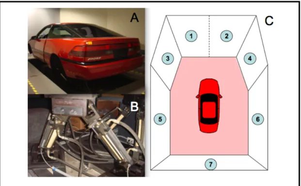
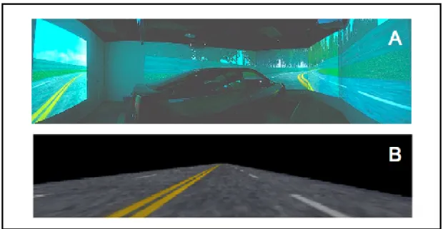
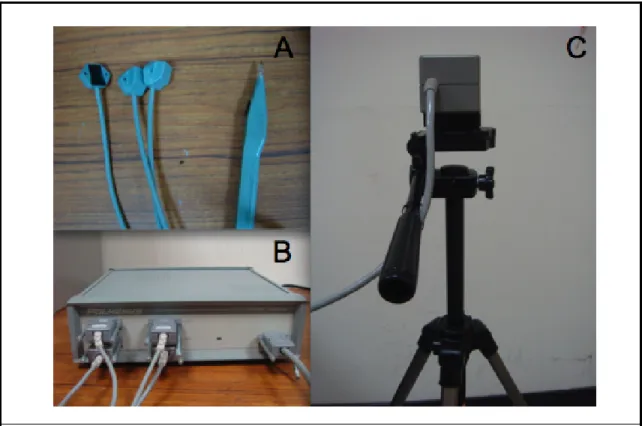
For safety concern, a 3D virtual reality-driving simulator was built to simulate real-life driving environment. A real car body was mounted on a six degree-of-freedom (DOF) Steward motion platform, which simulated the vibration caused by uneven road surface as well as kinesthetic force during real-life driving (Figure 1-A 1-B). In addition, the temperature, background illumination and other unexpected stimuli or distraction were under control to access the better EEG signal. The VR-based high way scenes were generated from seven personal computers which synchronized by the internet connection and then were projected to seven screens via seven projectors (Figure 1-C). These large screens generate an immersive sensation and near real-life driving environment (Figure 2-A).

(15)

8

(16)

Figure 2.The view of 3-D virtual reality environment.

2.3. Experimental paradigm

2.3.1. The event-related lane-departure task

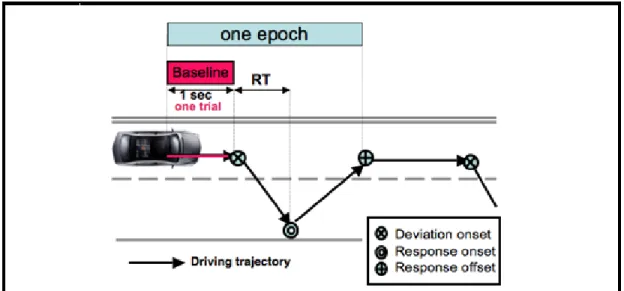
In the study, the driver’s drowsiness level was indexed by the event-related lane-departure task [53]. The VR scene which can properly emulate a car driving at a constant speed of 100 km/hr on the third lane of a 4-lane highway at night by refreshing 60 times per second (Figure 2-B). There were not acceleration and brake function in the car, so all the subjects had to do was controlling the steering wheel. The car was randomly drifted away from the center of the cruising lane to left or right with equal probability, which was controlled and triggered from the WTK program, to mimic the consequences of a non-ideal road surface [54-56]. During the experiment, subjects were instructed to steer back to the center of the cruising lane as quickly as possible after they detected the deviation. However, if the subjects fall asleep or stopped responding to the deviation, the vehicle will

(17)

10

eventually hit the virtual curb on either side without crash and continue moving along the curb. After such non-responsive periods subjects resumed task performance without experimenter intervention. The next deviation event occurred randomly 5 to 10 s after the moment when the vehicle was back in the third lane. Three parameters were recorded via a synchronous pulse marker train recorded by the EEG acquisition system in parallel, the onset of deviation, the subject's response onset and response offset (Figure 3). The deviation onset is recorded the moment that the car started to drift away. The onset of subject's response is defined as the moment that the subject turned the steering wheel to fix the deviation to the center of the third lane. The last one, response offset, is defined as the moment when the vehicle return to the center of cruising lane and the subject ceases to turn the wheel. Each complete single epoch included the three parameters in this task and started at the beginning of baseline. The baseline meant the duration of 1 second before the deviation onset, and the response time (RT) was calculated the period from the deviation onset to the response onset. Such experimental design allows the observation of continuous transition from complete alertness to deep drowsy states, and the baseline part without interference of muscle controlling could be used for analyzing the brain network.

(18)

Figure 3. A bird’s eye view of the event-related lane-departure paradigm.

2.4. Data acquisition

2.4.1. EEG data

2.4.1.1. Channel location measurement

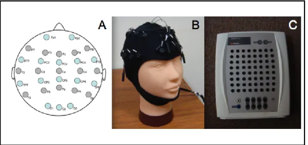
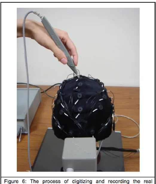
The brain activities from subject's skull were recorded by Ag/AgCl electrode cap with 30 channels (plus 2 references). The texture of cap was elastic and attached to an adjustable strap, and therefore it could totally cover subject's head without discomfort. All channels were arranged base on the modified International 10 - 20 system (Figure 4-A and 4-B). For accessing the actual location of each channel, each channel was redigitized by the 3D digitizer (Fastrak®, Polhemus, Figure 5) to reconstruct individual subject’s head model by the mathematical algorithms [57] for localizing the sources of brain activities.

(19)

12

(20)

(21)

14

(22)

2.4.1.2. Amplify the EEG signals

It is necessary to minimize the contact impedance of each electrode for increasing signal to noise ratio and diminishing the external noise integrating during the EEG recording. For this purpose, the conductive gel (Quik-GelTM, Compumedics NeuroMedical SuppliesTM) was carefully filled into each channel. The contact impedance of the EEG electrodes was controlled under 5kΩ before each experiment. Furthermore, the collected EEG activities were amplified by the Neural Scan Express System (NuAmps, Compumedics Ltd., VIC, Australia, Figure 4-C) and then recorded at 500 Hz sampling rate.

2.5. Data analysis

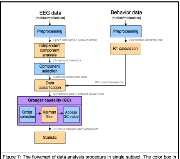
The data analysis flowchart in this study was shown in Figure 7. The motion and motionless data of each subject were generated a set of causal relationship by the analysis procedure respectively. Both EEG data and behavior data had to be preprocessed at first for rejecting those abnormal trials and artifacts. In the next step, EEG data were applied independent component analysis (ICA) for searching out the source data under 30 EEG channels, and on the other hand, the RT of each trial was calculated for EEG drowsy level classification. The third step in EEG data analysis, only interesting components were chosen to do further investigation, and then the drowsy levels, drowsy stages, of these components data were classified by RT in step 2 of behavior data. After those processes, we could apply the main algorithm, Granger causality (GC) which was indicated by purple block in figure 7, to the component data in the fifth step. There were 3 sub-steps in GC algorithm: order selection, Kalman filter and GC value accession. In the last step, the significant GC value was obtained after statistical testing. The causal relationship of each component in different drowsy levels could be realized after all these steps. The details of each process would be interpreted in following sub-chapter.

(23)

16

Figure 7. The flowchart of data analysis procedure in single subject.

2.5.1. Preprocessing

There were four steps in preprocessing: Integration of EEG and behavioral Data, reaction time, epoch extraction and artifact removal. Because driving trajectories and EEG signals were recorded by the different equipments (VR scene computer and Neuroscan respectively), we had to align these data by the triggers recorded in both machine first. Then the RT as defined in the event-relate lane departure [53] in each trial could be accessed by the driving trajectories. Third, the epochs were time-locked to 1 sec before deviation onset

(24)

from EEG data, which were referred as baseline. The last step, the abnormal trials in behavior data and EEG data had to be discarded before further analysis. Including the trials with RTs less than 0.3 sec, the overshoot or zigzag trajectories when subject reacted to car shifting, with extreme values in EEG channels and with severe fluctuations across most EEG channels were be abandoned.

2.5.2. Independent Component Analysis (ICA)

In this study, the inter-connection of those functional EEG sources was the intention to investigate. However, since the volume conduction of the skull and scalp tissue [58], the signal recorded from individual electrode is easily mixed with signals generated from other brain regions or which are not located at the position around the electrode or other sources outside of our brain, including the eye-movement (EOG), eye-blinking, muscle-movement (EMG). For approaching the more corrected brain sources from the mixing EEG signals which were from the experimental electrode and removing the unrelated signals to obtain the pure neural activities, we applied the ICA algorithm (the runica function of the EEGLAB toolbox) on the EEG signals to separate these mixing signals from source signals in each subject.

The independent component analysis is widely used for blind source separation problem [59-61]. There were four basic assumptions in ICA theorem: First, the source signals (neuron activities) were independent to each other and the correlation between each two sources was zero or close to zero. Second, the propagation delay from sources to sensors was negligible. Third, the sources were analog and the possibility density function (p.d.f.) was not the gradient of a linguistic sigmoid. Fourth, the summation at scalp electrodes of potentials arising from different brain areas was linear [62]. The ICA model is:

(25)

18

Where A was a linear transform called an m∗ n mixing matrix and S t

( )

= s t

[

( )

₁ ... s t

( )

_n

]

were statistically mutually independent. This ICA model described how the observed data were generated by a mixing process of the component vectors si. The independent component vectors si (often abbreviated

as ICs) were latent variables which could not be directly observed. The mixing matrix A is assumed to be unknown. All we observed were the random variables

X t

( )

= x t

[

( )

₁ ... x t

( )

_m

]

T, and the task of ICA was is to transform the observed

vectors xi, using a linear static transformation matrix W as:

U t

( )

= W ∗ X t

( )

(2)

A linear mapping W was from ICA such that the unmixed signals U(t) are statically independent. ICA was done by adaptively calculating the w vectors and setting up a cost function, which either maximizes the nongaussianity of the calculated S_k = w

(

T ∗ x

)

or minimizes the mutual information. In some cases, a priori knowledge of the probability distributions of the sources could be used in the cost function. After ICA training, we can obtain N ICA components U(t) which was very close to the real source activities S decomposed from the measured N-channel EEG data X(t).

 U(t)= u t

( )

₁T u t

( )

₂T  u t

( )

₃₀T               = W ∗ X t

( )

= w_1,1 w_2,1  w_30,1             ∗ x1(t)+ w_1,2 w_2,2  w_30,2             ∗ x2(t)+ + w_1,30 w_2,30  w_30,30             ∗ x30(t) (3)

(26)

2.5.3. Component selection

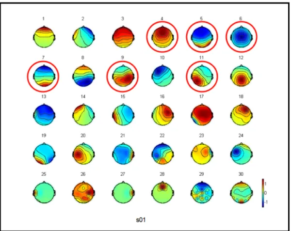
The scalp maps of each component represented the relative weight to compose from the channels (Figure 8). The maps from individual subject were generated by using the function topoplot of EEGLAB toolbox, which principle was rendering a column of the inverse of ICA weighting matrix onto the scalp (3). It was also revealed the spreading of the component topography.

In this study, there were six sources generated from the frontal area, supplementary motor area (SMA), somatomotor area, occipital midline area and bilateral occipital area to be submitted for the further analysis [62], as shown in figure 8. Figure 8 shown the 30 isolated scalp maps from the subject 01, and the components in red circle represented which were selected to analyze by Granger causality. The component 2, 3, 4, 5, 6 and 7 were frontal, SMA, right somatomotor, left somatomotor, occipital midline and bilateral occipital areas respectively.

(27)

20

Figure 8.An example of topographic maps of 30 independent components.

2.5.4. Data classification

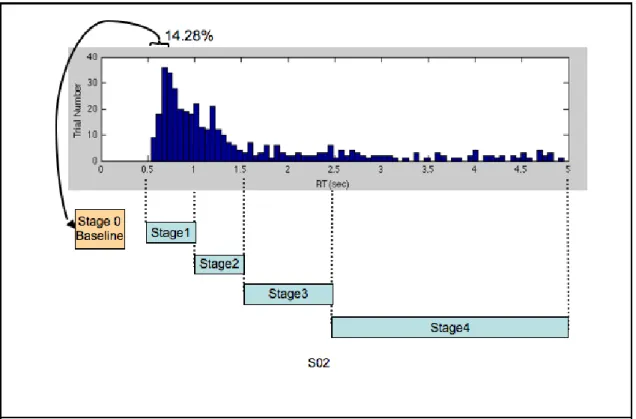
For observing the brain network in different drowsiness level, the criteria of different drowsiness level were defined to classify the EEG activities. The trial respective RT of the event-related lane-departure task was the basis in this study. If subjects stayed conscious, they could turn the car back more quickly which meant the RT would be shorter; and vice versa. All the data trial of one subject were segmented to 4 different stages from alertness to drowsiness (Figure 9). For decreasing the trial number difference between each stage, the stage length was not equal from 0.5 second to 1 second. All subjects was kept in alert state in the most of time, that majority of the distribution was centered on the range of RT

(28)

less than 1. The segments before RT=1.5 which represented as stage 1 to stage 2 were shorter, stage length were 0.5 second. However, the trial number decreased along with the increase of RT as RT>1.5. The stage length of stage 3 and stage 4 should be larger than 0.5 second for engaging the trial number in one stage to avoid unreasonable analysis. The stage 0 was regarded as baseline for statistical testing. The baseline had to keep in the most alert state and be controlled under reasonable trial number. Therefore the length of stage 0 was segmented as the first 14% alert trial instead of being segmented by RT for eliminating the difference in all subjects.

Figure 9. The diagram of stage segment in S02. The dark blue bars shown the distribution of trial number and RT.

(29)

22

2.5.5. Granger causality

For perceiving the connectivities in human brain under drowsiness state and alert state, we used Granger causality algorithm to obtain their causal relationship. The concept of causality was expressed by Granger for econometric purpose [43]. It based on the notion that causes imply effects during the future evolution of events and, conversely, the future cannot affect present. Granger causality assumed one time series y(t) caused another time series x(t) if y(t-1),y(t-2),...,y(t-p) participation in prediction of x(t) could significantly improves. The t was time point and p was order. Therefore, the basic assumption of Granger causality was that the participating time series must be autoregressive model (4). In multi-channel EEG data, there was a time-variate multivariate autoregressive model (tvMVAR) to fit all time series [64]. Consider a set (K components) of processes like Xt represented as:

Xt = At−1∗ Xt−1+ + At− p∗ Xt− p+ Et₍₄₎

where, t represented the current time point, Xt, Xt−1,, Xt− p_{were K x 1 observed}

data matrix, p was model order, and E was a zeros mean Gaussian noise vector.At−1,, At− p _{were K x K coefficient matrix of tvMVAR, and it also}

represented as linear time-lagged dependence. At a given time, the diagonal elements of A represented the self-connectivity of each channel, and off-diagonal element represented the inter-connectivity between each channel. If the prediction of Xt of α component was more accurate by adding a specific

component β, we could say, component β caused component

α

. In other words, If the error matrix Et was controlled in the minimum, the coefficients of

component β to complete component

α

indicated how much the β caused the

α

. The following 4 section, order selection, Kalman filter, Granger causality value and statistical testing were 4 steps to determine if there was any connection exist between two time series components. The purpose of the first three steps was

(30)

accessing the coefficients of observed data and analyzing the strength of causal relationship between each component in each time sample and different drowsy stage. The statistical testing was used to determine the causal relationship was established or not.

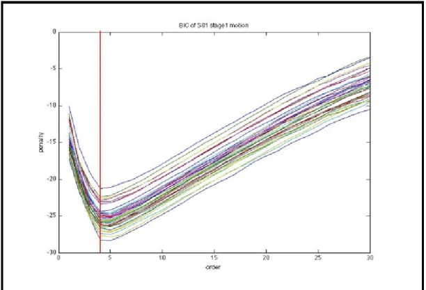
2.5.5.1. Order selection

Before accessing the observed measurements model coefficients, selecting the model order to get the best prediction was necessary in each different drowsy stage GC analysis. The Bayesian information criterion (BIC) [65] function was used to choose the model order p to yield a well-fit tvMVAR. The penalty was of each order calculated by BIC criterion, and selected the model order for which BIC penalty reaching for a minimum.

BIC p

( )

= dep + log tn

( )

∗ p /n (5)

where, p was the model order presenting the current order, de was the predict error of p order, tn was the trial number of the observed data, n was the sample number of this trial. The error of observed data model prediction, de, was computed by QR decomposition algorithm which was often used to solve the linear least square problem. Therefore the de value had to be accessed once as calculating the p order each time. The BIC value of order p was the penalty of the observed data model prediction, that is, the lower value meant the better prediction and the more well-fit generated model.

(31)

24

Figure 10.The BIC testing in subject 01 (S01) with 36 trials.

Figure10 shown that the shape of the curve was greatly similar in all trials from one subject. The order with the lowest penalty would be selected to be the model order as the red circle in figure 10. In the example, 4 was selected to be the model order for predicting the model coefficients in the next step.

2.5.5.2. Kalman filter

Figure 11 showed the following steps of Granger causality analysis after order selection in an example of bi-variate. Applying Kalman filter was the next step. The purpose of Kalman filter was to use measurements that are observed over time that contain noise, random variations, and other inaccuracies, and produce the model whose values that tended to be closer to the true values of the measurements and their associated calculated values [66,67]. In GC analysis,

(32)

the advantage of adaptive filter such as Kalman filter was that the autoregressive model of observed data could be variable. Kalman filter could detect the change of linear combination of model along with time series in each prediction, therefore the assumption of stationary input data was unnecessary and one set of model coefficients was accessed in each time sample [68]. Otherwise, Milde et al. [51] reported that this adaptive way to access the model coefficients was more suitable than recursive least square (RLS) [69], which was the other adaptive filter used in GC analysis.

The procedure of filtering was producing estimates of the true values of measurements and their associated calculated values by predicting a value, estimating the uncertainty of the predicted value, and computing a weighted average of the predicted value and the measured value. The estimates produced by the method tend to be closer to the true values than the original measurements because the weighted average has a better estimated uncertainty than either of the values that went into the weighted average. Assume there was a m-dimensional vector autoregressive model of order p, and those functions could be shown as below:

Y t

( )

= H t

( )

∗ X t

( )

+ε

( )

t (6) X t

( )

= Γ t

( )

∗ X t −1

( )

+ W t

( )

(7) Κt = Ρt|t−1∗ H t

( )

T ∗ H t

[

( )

∗ Ρt|t−1H t

( )

+ R t

( )

]

−1 (8) Ρ_t|t = Ρ_t|t₋₁− Κ_t∗ H t

( )

∗ Ρ_t|t₋₁ (9) ε

( )

t = Y t

( )

− H t

( )

∗ Xt|t−1 (10) Xt+1|t= Γ t

( )

∗ X

[

t|t−1+ Κt∗ε t

( )

]

(11) Ρt+1|t= Γ t

( )

∗ Ρt|t∗ Γ t

( )

+ Q t

( )

(12) X_0|−1= X₀ (13)  Ρ_0|−1= Ρ0= 0  0    0  0           (14)

(33)

26

where, t was the current time point, Y t

( )

was the observed data, H t

( )

was the observed measurement matrix with dimension m∗ m2

p , X_t was the m2

p∗ m2

p

state variable matrix, and it also represented the model coefficient matrix in this study. Γ t

( )

was the transition matrix whose size was also m2p∗ m2p, and it was identical matrix for assuming the coefficients evolve according to random walks.

Kt was the Kalman gain matrix, Ρt|t was the priori covariance matrix of the

estimation error, Ρt+1|t was the posteriori covariance matrix, R t

( )

was the

observation noise covariance, R t

( )

=ε∗εT , W t

( )

was the zero-mean white process-noise, Q t

( )

was the state-noise covariance. The function 6 and 7 were basic state-space form. Y t

( )

and H t

( )

were known observation data, and the aim of Kalman filter in this study was to estimate the model coefficients Xt by Y t

( )

and H t

( )

, in the other words, to access the function 6. Function 8, 9 and 10 were the innovation part in the filter preparing for next time point prediction, and function 11 and 12 were prediction part. The filter trained the observed data time sample by time sample, and then the object coefficient matrix Xt at each time

(34)

sample time 1 sec significant GC value 0 125 250 0 125 250 filter filter

Moving window by 1 sample

Component A

window length = order

GC value GC value GC value GC value Component B A to B B to A

compare with stage 0 GC value distribution

significant GC value filter significant GC value significant GC value 0 -0.05 250 Comp A Comp B GC value non-zero > zero

?

Comp A Comp B Yes No No causal relationship sample filter

(35)

28

Figure 11. The diagram of Granger causality application of bi-variate time series after order selection.

2.5.5.3. Granger causality value

The original autoregressive model of observed data appeared to be analyzed by GC after filtering. We used a three components example to explain how to access GC value from the coefficient matrix Xt in function 6. Assume the

autoregressive model was solved by Kalman filter in previous section:

Y t

( )

= X i

( )

i=1 p

∑

∗Y t − i

( )

+ε t

_{( )}

(14)

The same with the function 6, Y t

( )

was the observed data with m components and t presented the current time point, p was the model order, Xi represented

linear time-lagged dependence which was referred as coefficient matrix from lag 1 to order p. For explaining legibly, the function 14 was simplified order to be equal to 1 and only three components, not only that, the equation was expanded as following function:

Figure 11: The diagram of Granger causality application of bi-variate time series after order selection. There were 2 components in this example, component A (comp A) and component B (comp B). Two components were trained by the Kalman filter which were represented as blue blocks with order length as window length to access the model coefficients. Next step was calculated the GC value in each time point by coefficients from filter represented by green blocks. Testing the significance was after the GC value calculating represented as pink blocks. Each GC value along with the time series was compared with the distribution of GC value in stage 0, if the value was in the distribution, the value was set for 0; else the value kept the original GC value. The last step of Granger causality was decision of the causal relationship. If the non-zero value was much more than the zero in the whole GC value along the time series, then the connection, causal relationship was established.

(36)

y1

( )

t y2

( )

t y3

( )

t           = x11 x12 x13 x21 x22 x23 x31 x32 x33           ∗ y1

( )

t−1 y2

( )

t−1 y3

( )

t−1           + ε1

( )

t ε2

( )

t ε3

( )

t           (15)

The diagonal elements, x₁₁x₂₂x₃₃ represented the self-connectivity at lag 1, and the others were inter-component connectivity at lag 1. These coefficients were positive relation with causal relationship in above coefficients matrix. For instance,

y₁

( )

t was composed by y₁

( )

t−1 y₂

( )

t−1 y₃

( )

t−1 with coefficients x₁₁x₁₂x₁₃

respectively, that mean the relative strength of influence from component y₂toy₁

at time point t-1 was expressed by the ratio abs x

( )

₁₂ / abs x

( )

₁₁ + abs x

( )

₁₂ + abs x

( )

₁₃ , and from y3 was expressed by the ratio abs x

( )

13 / abs x

( )

11 + abs x

( )

12 + abs x

( )

13 .

Therefore the GC value was designed [70,71] :



GC t

( )

_comp1_{→comp 2}= i=1abs x

(

21

( )

i

)

p

∑

abs x

(

11

( )

i + + xm1

( )

i

)

i=1 p

∑

(16)

2.5.5.4. Statistical testing

For the difference in time-space and the EEG variance from person to person, the statistic testing was trial by trial in each subject. The EEG data in stage 0, baseline, were regarded as reference for the GC value in stage 1 to 4 to test the significance. All the single GC values along with time series were compared with the distribution of stage 0 distribution, if the GC value from stage 1 – 4 wasn’t in the 95% confidence interval of stage 0, the GC value was significant and the GC value was kept, else the GC value was set for 0. Since avoid influence of the extreme value from minor trial, the median were used to average all the trials. After the median accessing, only if number of non-zero GC values were much more than the number of zero in whole time series between two components, the causal relationship in these two components was established as the example of connection of comp A to comp B in figure 11.

(37)

30

2.5.6. Power spectrum analysis

Previous studies suggested that drowsy EEG dynamics could be observed from two different aspects, the tonic and phasic changes [72, 73] and both aspects were processed by frequency analysis. Phasic change referred to the EEG power triggered from stimulation by the specific events, like the deviation onset in our experiment. Time-frequency was used to investigate the change of power spectral in grouping data from deviation onset to deviation offset. On the other hand, the tonic changes referred to the converting of baseline power spectral associated with change of cognitive state such as the different drowsy stage in this study. The baseline data were transferred to power spectral in each stage to observer the tonic changes from alert state to drowsy stage.

2.5.6.1. Event-related spectrum perturbation (ERSP)

Time-frequency transform is a spectrotemporal decomposition technique to analysis the event-related data perturbations in spectral domain of EEG channel data or component data [74]. For assessing the EEG activities during the stimulation and after the response in different drowsy stage, the epochs of each stage from all subjects were extracted from -1 ~ 7 seconds to estimate the changes of ERSP. The 2000 points in each observed component epoch was chronically divided into 200 overlapped sub-windows with 250 points, and the power spectrum of each sub-window was computed by discrete wavelet transforms (DWT) using newtimef() function of EEGLAB [73]. The frequency bins respective to the 200 sub-windows that distributed in -1 to 7seconds were obtained stage by stage. In the last step, we average the frequency bin in all the epochs in one stage to realize the ERSP changes from deviation onset in each drowsy stage.

(38)

Figure 12. The diagram of time-frequency transform of ICA component activity in an epoch.

2.5.6.2. Tonic power spectrum

Tonic data were the main source for Granger causality to assess the brain network in different drowsy stage because we assuming there were not unexpected brain activities or event in this duration. Therefore the state were stable in whole baseline, the power spectrum should also be stable. Each observed component baseline with 250 samples from all subjects was directly computed the power spectrum by fast Fourier transforms using fft() function in MATLAB stage by stage. The power respective to frequency in each component and each stage was obtained. Then we computed the average value from all trials by the frequency power in different drowsy stage to observer the tonic changes from alert state to drowsy stage.

(39)

32

3. Results

3.1. Behavioral data

The information of behavior data were shown in Table 1 and Table 2. Table 1 showed the different 4 drowsy levels and the respective RT. Table 2 showed the trial number in each stage and the average reaction time of behavior data. The stages number from 1 to 4 represented the subject’s alert status to drowsy status with inconsistent length of RT. The trial distribution in table 2 revealed that the subjects kept in the alert status at most of the time, and therefore the length in stage 1 and 2 were shorter than stage 3 and 4 to balance the difference of trial distribution. The last row indicated the average RT of each stage including the motion and motionless condition.

Table 1: The Stage no. and the Respective RT

Stage no.

Baseline

1

2

3

4

RT (SEC.) The First

14.28%Trials 0.5 - 1 1 – 1.5 1.5 - 2.5 2.5 - ∞

(40)

Table 2: Trial Number and RT of Behavior Data Subject Index Trials in Stage 0 Avg. RT (SEC.) Trials in Stage 1 Avg. RT (SEC.) Trials in Stage 2 Avg. RT (SEC.) Trials in Stage 3 Avg. RT (SEC.) Trials in Stage 4 Avg. RT (SEC.) Total Avg. S01 45 0.65 196 0.77 66 1.21 19 1.74 37 6.62 1.60 58 0.69 142 0.82 36 1.12 27 1.85 38 4.84 1.33 S02 67 0.65 183 0.76 108 1.18 58 1.95 120 5.49 2.23 37 0.90 41 0.90 137 1.16 62 1.82 23 4.50 1.59 S03 62 0.84 79 0.86 236 1.24 108 1.70 11 4.43 1.38 24 0.59 135 0.71 8 1.01 5 1.25 19 11.66 2.03 S04 40 0.71 96 0.82 109 1.21 54 1.77 23 8.56 1.81 45 0.74 109 0.82 80 1.19 38 1.85 92 8.34 3.25 S05 61 0.55 135 0.78 100 1.19 64 1.80 109 5.85 2.33 44 0.68 139 0.81 55 1.11 22 1.78 92 17.09 5.87 S06 36 0.44 168 0.64 21 1.16 6 1.37 14 18.07 1.68 35 0.59 199 0.71 17 1.07 4 1.55 29 9.89 1.85 Avg.

-

0.64

-

0.77

-

1.20

-

1.72

-

8.17 2.25 0.70 0.80 1.11 1.68 9.39

The pink parts were indicated the motion condition, and the white parts were the motionless condition.

Tables 2. Trial Number and RT of Behavior Data.

3.2. Brain network of single subject data from

alert stage to drowsy stage

Figure 13 showed the brain connectivity from stage 1 to 4 of S06 in simulated real driving situation. The graph showed the propagations of the 6 components from alert status to drowsy status. Those components were represented by different color, the frontal area was represented by the red dot,

(41)

34

the SMA was orange dot, right and left somatomotor area was yellow and green dot respectively, the occipital midline was blue dot and the bilateral occipital was purple dot. The position of components and the strength of GC connections were indicated in the right bottom of figure. All the connections between any two components had been tested the significance by GC value.

In the S06 case, the most of connections influence were weak in stage 1. The connections got stronger from stage 2, and it was clear that the frontal area received all the information flow from each components except the midline occipital area which also received the information flow from other components, but slighter than the frontal area. However, the propagations of information flow, or causal relationship, was changing in stage 3. In stage 3, the strength of connections was deadened and the afflux was not the frontal area or the midline occipital area. The causal connectivity related to right and left somatomotor areas were becoming dynamic in this stage, and some influences were into the bilateral occipital area. The last stage, stage 4, those connections were similar to those in stage 1 or 2, the afflux were centered on frontal area and occipital area, but the strength of connection was different, the stronger connections were into the occipital areas instead of the frontal area. In this stage, the flow direction of causal relationship was more consistent than in other stage.

(42)

Figure 13. The brain connectivity of S06 from stage 1 ~ 4 in simulated real driving.

3.3. Brain network of grouping data from

alert stage to drowsy stage

In order to observe the consistence in each subject, the integration of brain network of 6 subjects was shown below. For keeping the difference of baseline from person to person, the causal relationships were accessed by single subject instead of clustering all the trials to do GC analysis. Afterwards, the connection between two components appeared over 3 subjects at the same stage, and it would be selected and shown in the Figure 14 ~ 16. This grouping way could keep the reliability of reference of statistical testing.

(43)

36

3.3.1. Brain network in 3D coordinates

In results of grouping data, the dipoles were fitted to 3D talairach coordinates model to present the brain network. The coordinate was indicated in the right side of Figure 14, and the three surfaces were left to right, anterior to posterior and superior to inferior of human brain. As shown in Figure 13, the six components were represented by different color dots respectively in Figure 14, and those dots also projected to the three surfaces with a half dot to indicate, and therefore the EEG equivalent-dipole locations and orientations of human brain were visualized

Figure 14. The brain network in 3D coordinates.

3.3.2. Brain network in stage 1

The results of stage 1 were shown in Figure 15-A. Subjects should stayed in very alert status in this stage for the respective RT was 0.5 ~ 1 second. In stage 1, the signal flow sent to frontal area, SMA and midline occipital area, especially the frontal area. All components sent signals to frontal area excepting the SMA, and SMA received the signal flow from occipital areas. On the other hand,

(44)

midline occipital received the signal flows from two somatomotor areas. Generally, the trend of signal flow was directing to the anterior part of brain from posterior part in stage 1, and somatomotor areas sent to both frontal and midline occipital area.

Figure 15. The brain networks of grouping data in stage 1 and 2 (motion condition).

3.3.3. Brain network in Stage 2

The respective RT was 1 ~ 1.5 seconds in stage 2, and we showed the results in simulated real driving (motion condition) in Figure 15-B. The trend was still towards frontal, central and midline occipital area, and the directions of connection centered on frontal area much more than previous stage. The signal flow from somatomotor did not send to occipital midline area, only sent to the anterior of human brain. And the signal flow from bilateral occipital area to SMA in stage 1 shifted to midline occipital area in this stage. It is clearly that the main destinations of signal flows were frontal area and midline occipital area which inheriting the previous stage.

(45)

38

3.3.4. Brain network in Stage 3

There were many changes in stage 3 whose RT was 1.5 ~ 2.5 seconds. The main concentration of signal flow was not frontal area anymore, but was occipital midline area. In Figure 16-A, there were three components sending information to midline occipital area and two sending to SMA and left somatomotor area. The midline occipital area collected the most connections clearly. There had been four connections concerning frontal area in previous stage, but only left one, midline occipital to fontal, in stage 3. Frontal area became a signal source in this stage; it sent signals to SMA area and left somatomotor area. The SMA received the signal flows from frontal area and right somatomotor area, and seemed like the destination of signal flows shifted to posterior brain gradually. The sending of somatomotor area was back to midline occipital area and SMA, and somatomotor received the signals from midline occipital area. Stage 3 was the turning point of signal transmission from alert state to drowsy state, and it was different explicitly. The effect of frontal area was reduced and the somatomotor area and midline.

(46)

3.3.5. Brain network in Stage 4

In the last and most drowsy stage, which RT was more than 2.5 seconds, the brain network inherited the previous stage and the direction of signals centered on midline occipital area much more. In Figure 16-B, we could observe that the major arrows directed to posterior brain, that was, the occipital area. The midline occipital area received signal flows from all of the components except frontal area, and bilateral occipital area also received three causal relationships from three components SMA, right somatomotor, and including the frontal area. All causal relationships were towards to posterior brain, but there was one arrow directed to anterior part of brain, the bilateral occipital area to frontal area. The concentration of brain networks transferred to occipital area obviously, especially in the midline occipital area, beside that, the opposite location, frontal area, also received the signals from bilateral occipital. The main effect in drowsy stage was midline occipital area, which received those signal flows and didn’t send to any component. It was quite different with the brain network in alert stage such as stage 1 or 2.

3.4. The comparison of brain network in

motion and motionless condition

This section showed the comparison of brain network in motion platform and motionless platform. We used two kinds of simulator to represent the difference from reality and laboratory condition. The brain networks in motionless condition explain the brain networks from alert stage to drowsy stage only with the visual stimulation. Although the design of experiment was not similar with the real driving, the influence of consciousness was more remarkable. The kinesthetic stimulation was an extra input in motion condition for simulating reality situation, and therefore we indicated the connections only in motion condition to elucidate the influence on causal relationship from the extra input. In each stage, there were 3 brain networks in Figure 17 ~ 20 respective to motion, motionless

(47)

40

condition and the comparison. The parts of motion condition were the same with which in Figure 14 ~ 16, and in comparison, the consistent signal flow represented by blue arrows in both condition and those inconsistent parts by red.

3.4.1. The comparison of brain networks in stage 1

The concentration of signal flow was frontal and midline occipital area in motion condition, however, it only sent to frontal area in motionless condition. And the number of connections in motionless were fewer than in motion condition, the brain network was more definite. In the comparison, all the connections in motionless condition were the consistent part in stage 1, and it expressed that the frontal area was caused by the four components, which two somatomotor and two occipital areas, in both condition. The consistent trend was from posterior to anterior brain. However, there were lots extra connections in motion condition, and those almost were concerned in SMA and midline occipital area. We could find out the SMA and occipital midline area did not participate in motionless condition.

(48)

Figure 17. The brain network in stage 1.

3.4.2. The comparison of brain networks in stage 2

The destination of signal flow still was frontal and midline occipital area in motion condition, but the effect of SMA was decreased. In motionless condition, the brain network was very like the one in stage 1, nevertheless, the causal relationship from somatomotor area was replaced with from the SMA. In comparison part, the most of those connections sent to frontal area were keeping consistent, and there were connections about somatomotor area and midline

Figure 17: The brain network in stage 1. In motion condition, the signal flows were sent to frontal, SMA and midline occipital area, but only the signal flows were only sent to frontal area in motionless condition. In comparison, the connections linking the central and midline occipital were extra in motion condition.

(49)

42

occipital area belonged to inconsistent part. The direction of inconsistent connection was different with previous stage. Somatomotor area sent the signal flow to anterior brain, and the bilateral occipital sent to midline occipital area.

Figure 18 The brain network of stage 2.

3.4.3. The comparison of brain networks in stage 3

The brain network was quite different in both motion and motionless condition. The main destination was not the frontal region, but was midline

Figure 18: The brain network of stage 2. The trends were still towards to the frontal, SMA and occipital midline area, but the somatomotor area sent the signal flow to frontal area instead of occipital midline area in motion condition, and fewer connections were towards to SMA. In motionless, the SMA sent to frontal instead of left somatomotor area sending. The trend was expanded from the previous stage: Consistent parts of comparison were those signal flow sent to frontal area, and inconsistent parts were those sent to SMA and midline occipital area.

(50)

occipital area. In motion experiment, the signal flow sent to midline occipital much more than stage 2, and the somatomotor area also received massage in this stage. In the other side, the motionless condition, the signal flows were centered on midline occipital area obviously, from bilateral occipital and SMA. In previous stage, there were four connections linking with frontal area, but there was none in stage 3. Although the two conditions also changed the concentration from anterior brain to posterior brain, the consistent part in comparison was only one connection, SMA to midline occipital area. There were many connections in inconsistent part, those about the left and right somatomotor area and the frontal area. The somatomotor area did not generate any causal relationship in motionless, but they were active in motion condition. That was the biggest difference in this stage.

(51)

44 Figure 19. The brain network of stage 3.

Figure 19: The brain network in stage 3. Both in motion and motionless condition, the main destination of signal flow was not frontal area, but was occipital midline area. The causal relationship seemed to shift to posterior part gradational in motion condition, and seems like had shifted in motionless. In comparison, there were many difference which about the left and right somatomotor area and the frontal area.

(52)

3.4.4. The comparison of brain networks in stage 4

In the drowsiest stage, the concentration of brain networks transferred to occipital area obviously, especially in the midline occipital area, beside that, the opposite location, frontal area, also received the signals from bilateral occipital in motion condition. The brain network in motionless condition was similar with the previous stage, but the concentration was stronger. All the signal flows were sent to midline occipital area, and only one somatomotor area did not work. In the comparison part, the consistent connections were sent to midline occipital area, and the inconsistent connections were including the left somatomotor area to midline occipital area, those sent to bilateral occipital area and the bilateral occipital to frontal area in motion condition.

(53)

46 Figure 20. The brain network of stage 4.

Figure 20: The brain network in stage 4. The brain network extended the previous stage and centered on midline occipital area. In motion condition, the midline and bilateral occipital area received connections from all of the components, and the midline occipital area in motionless also receive the most signal flows. However, the connection were more complex in motion condition, the signal flow did not only send to midline occipital area, but also to bilateral occipital and frontal area. Beside that, the both somatomotor area were active in motion but not in motionless condition.

(54)

3.5. Summary

Figure 21-A showed the concentration of brain networks from alert to drowsiness in motion and motionless condition. From alert to drowsiness, the concentration of signal flows shifted from frontal area to midline occipital area. This phenomenon was more obvious in laboratory situation than reality situation. There were a lot kinetic stimuli in real life like motion condition to make the brain networks more complex to be illustrated. Figure 21-B showed the power spectrum of midline occipital component in different drowsy stage in both two conditions. The power of alpha band increased along with drowsy level, as in brain networks, the phenomenon was more obvious in motionless condition.

(55)

48

Motionless

Motion

Alert

Drowsiness

Stage 1 RT: 0.5 - 1 Stage 2 RT: 1 - 1.5 Stage 3 RT: 1.5 – 2.5 Stage 4 RT: >2.5

Alert

Drowsiness

A

B

(56)

Figure 21: The concentration of brain networks and EEG power spectrum in motion and motionless condition. 21-A: The destination of signal flows shifted from frontal area to midline occipital area with subject’s consciousness. Brain networks in real life condition were more complex than laboratory condition for extra kinetic stimulation. 21-B: The power spectrum of occipital component respective drowsy stage. The power of alpha band increased along with drowsy level, as in brain networks, the phenomenon was more obvious in motionless condition.

Figure 21. The trend of brain networks and EEG power spectrum in motion and motionless condition.

(57)

50

4. Discussion

The aims of this study were to determine the brain connectivity between different brain regions from subject’s alert status to drowsiness status and to compare the above brain network in motion and motionless simulation, finding the influence of kinesthetic input on EEG signal flows in reallife. The results in previous chapter showed the brain networks in each stage and the consistent and inconsistent part in comparison of motion and motionless conditions. From alert stage to drowsy stage, the concentration of signal flow shifted from the anterior brain to the posterior brain. In addition, there were more connections supposed to be including kinetic stimulus in motion condition than in motionless condition. Figure 22 showed the structure of signal flows summarized from Figure 21 to illustrate the finding clearly.

Motion

Motionless

Stage 1 RT: 0.5 - 1 Drowsiness Stage 2 RT: 1 - 1.5 Stage 3 RT: 1.5 – 2.5 Stage 4 RT: >2.5 Alert

(58)

Figure 22: The dendrogram of brain networks from drowsiness to alert in motion and motionless condition. The structure illustrated the concentration of brain network and the difference between two conditions. Stage 1 and 2 seemed like the same status, and the enormous change appeared in stage 3. In addition, stage 4 was expanded from stage 3. The involving components and connections in motion condition were much more than motionless condition. It illustrated the brain networks were influenced by more inputs in real-driving simulation.

Figure 22. The dendrogram of signal flow from drowsiness to alert in motion and motionless condition.

4.1. The brain network from alert state to

drowsy state

4.1.1. The concentration of brain networks

In Figure 23, the green line represented the consistent part of brain networks in motion and motionless condition. Most connections in motionless also occurring in motion condition explained that it caused by drowsiness level. Frontal area was the main region to receive signal flows from other posterior components in stage 1 and 2, but the trend totally changed in next stage. The destination was not frontal area in stage 3; most signals were sent to midline occipital area. In addition, the connections directed to midline occipital more obviously in stage 4. The trend was that sending to frontal area in alert stage and then sending to occipital area since into drowsier stage.

駕駛在不同瞌睡程度下大腦訊號傳遞網絡的變化

國 立 交 通 大 學

多媒體工程研究所

碩士論文