電子系統層級上的設計方法－以正交多頻多工系統為例

全文

(1)國立交通大學電子工程學系碩. 電子研究所碩士班士. 論. 文. 電子系統層級上的設計方法－以正交多頻多工系統為例. Design Methodology at Electronic System Level: A Case Study of OFDM System. 研究生：陳冠豪指導教授：周景揚博士. 中華民國九十五年八月.

(2) 研究生：陳冠豪. Student: Guan-Hao Chen. 指導教授：周景揚博士. Advisor: Dr. Jing-Yang Jou. 國立交通大學電子工程學系電子研究所碩士班碩士論文. A Thesis Submitted to Department of Electronics Engineering & Institute of Electronics College of Electrical and Computer Engineering National Chiao Tung University In Partial Fulfillment of the Requirements for the Degree of MASTER OF SCIENCE In Electronics Engineering August 2006 Hsinchu, Taiwan, Republic of China. 中華民國. 九十五. 年八. 月.

(3) 電子系統層級上的設計方法－以正交多頻多工系統為例研究生：陳冠豪. 指導教授：周景揚. 博士. 國立交通大學電子工程學系. 電子研究所碩士班. 摘要電子系統層級上的設計方法提供一種新風格的設計方法。這種設計方法的特性是可以在模擬時間和在模擬中所獲得的資訊間取得平衡。在這篇論文裡，我們以一個正交多頻多工系統為例，提出一種在電子系統層級上的設計方法，做有關設計的模型和設計空間勘查方面的工作，對系統效能作評估，並對實驗結果加以討論。我們依該方法在循序可執行程式碼和暫存器傳輸層級間建立抽象模型。它讓我們可以在短時間之內評估系統的效能並且萃取重要的資訊以及在能在設計流程中比較直覺的完成設計。. i.

(4) Design Methodology at Electronic System Level: A Case Study of OFDM System. Student: Guan-Hao Chen Advisor: Dr. Jing-Yang Jou. Department of Electronics Engineering Institute of Electronics National Chiao Tung University. Abstract Design methodology at electronic system level (ESL) offers a new style design methodology. It features high degree of balance between simulation time and information got from simulation. In this thesis, we use an orthogonal frequency division multiplexing (OFDM) system as a case study, apply a design methodology at ESL to do design modeling, design space exploration and performance evaluation and discuss these experiments.. We base on it to establish abstract model between the. sequential executable codes and the register transfer level (RTL) description. We are able to evaluate performance in relatively short time, obtain important information and complete the design more instinctively.. ii.

(5) Acknowledgment First and foremost, I would like to express my sincere gratitude to my advisor Professor Jing-Yang Jou for his suggestions and guidance throughout the years. As my advisor, he not only helped me on my work, but also gave me a lot of valuable advice on my life. I was such a lucky guy to have worked with him. Also, I would like to thank Cheng-Yeh Wang, Liang-Yu Lin; they were the first people I would go to whenever I needed support or to share my happiness and sorrow. Without their help, I wouldn’t have finished my work and learned so much. Special thanks to EDA lab and VSP lab members, for their company and friendship; it has been a great time to be together with them. Finally, I would like to express my sincere gratitude to my family and all my friends, who have always helped and encouraged me a lot.. iii.

(6) Contents 摘要.................................................................................................................................i Acknowledgment ......................................................................................................... iii Contents ........................................................................................................................iv List of Tables.................................................................................................................vi List of Figure................................................................................................................vii Chapter 1 Introduction ...................................................................................................1 1.1 Technology Tread.............................................................................................1 1.2 The focus of our work......................................................................................1 1.3 Related Works ..................................................................................................2 1.4 Thesis Organization .........................................................................................2 Chapter 2 Preliminary ....................................................................................................3 2.1 Refinement.......................................................................................................3 2.2 SystemC Features.............................................................................................4 2.3 Process Network ..............................................................................................5 2.4 The OFDM System ..........................................................................................6 Chapter 3 Our Platform..................................................................................................8 3.1 Coding Guideline of Sequential Executable Code...........................................8 3.2 A Process Network Model .............................................................................12 3.3 Timed Functional Model................................................................................17 3.4 Resource Management and Scheduling .........................................................20 Chapter 4 Experimental Results...................................................................................32 4.1 Experimental Information..............................................................................32 iv.

(7) 4.2 Experimental Results .....................................................................................34 4.2.1 Experiment..........................................................................................34 4.2.2 Performance Analysis .........................................................................40 Chapter 5 Conclusion and Future Work.......................................................................42 Reference .....................................................................................................................43 VITA ............................................................................................................................44. v.

(8) List of Tables Table 1 Experimental fundamental assumptions of timing..........................................32 Table 2 Experimental assumptions of architecture in experiment I.............................34 Table 3 Experimental assumptions of architecture in experiment II ...........................35 Table 4 Experimental assumptions of architecture in experiment III ..........................36 Table 5 Experimental assumptions of architecture in experiment IV..........................37 Table 6 Experimental assumptions of architecture in experiment V ...........................39 Table 7 Performance analysis ......................................................................................40. vi.

(9) List of Figure Figure 1 Refinement ......................................................................................................3 Figure 2 A directed graph representing a process network ............................................5 Figure 3 Transmitter architecture...................................................................................6 Figure 4 Receiver architecture .......................................................................................7 Figure 5 Channel estimation block ................................................................................7 Figure 6 An example of coding guidelines ....................................................................9 Figure 7 The data exchange of the code example........................................................11 Figure 8 SystemC code of a node of the process network...........................................13 Figure 9 The system top-view written in SystemC......................................................14 Figure 10 Receiver architecture divided into processes ..............................................15 Figure 11 Receiver architecture divided into processes...............................................16 Figure 11 Process network model of the OFDM system .............................................16 Figure 12 Process network model of the OFDM system (with two delay element)....17 Figure 13 SystemC code of timed functional model ...................................................19 Figure 14 Motions of resource scheduler I ..................................................................21 Figure 15 Motions of resource scheduler II.................................................................21 Figure 16 Motions of resource scheduler III................................................................22 Figure 17 Motions of resource scheduler IV ...............................................................22 Figure 18 Motions of resource scheduler V.................................................................23 Figure 19 The model of resource scheduling...............................................................24 Figure 20 The pseudo-code of resource scheduler ......................................................25 Figure 21 SystemC code of timed functional model with resource scheduling ..........27 vii.

(10) Figure 22 OFDM memory scheduling.........................................................................29 Figure 23 OFDM FFT scheduling ...............................................................................30 Figure 24 OFDM memory static scheduling ...............................................................31 Figure 25 OFDM execution time of experiment I (ms)...............................................34 Figure 26 OFDM execution time of experiment II (ms)..............................................36 Figure 27 OFDM execution time of experiment III (ms) ............................................37 Figure 28 OFDM execution time of experiment IV (ms) ............................................38 Figure 29 OFDM execution time of experiment V (ms) .............................................39. viii.

(11) Chapter 1 Introduction. 1.1 Technology Tread. As predicted by International Technology Roadmap of Semiconductors (ITRS), people are able to integrate billions of transistors on a chip within ten years. Current mainstream system-on-chip (SoC) designs do not yet fully exploit the 100 million transistors per chip possible with today’s mainstream silicon technology [1]. We see that design gap is a big problem nowadays. The increasing gap between silicon technology and actual SoC design complexities tell us that we need design methodology at electronic system level (ESL) to combine with intense use of off-the-shelf components [1]. Besides, more and more simulation time at register transfer level is just another big problem of these problems. Developing design methodology to balance simulation time and information got from simulation is helpful to design a modern system efficiently [2].. 1.2 The focus of our work. At this work, a real case study of design methodology at electronic system level is conducted. An OFDM system will be used for this case study. We will establish 1.

(12) design methodology at ESL, and apply it to this OFDM system. We specially focus on the difference between our design methodology and classic design methodology.. 1.3 Related Works. The most well known related work is Metropolis [3], which is designed to provide an infrastructure based on a model with precise semantics that remain general enough to support existing computation models and accommodate new ones. In our work, we apply our design methodology at ESL to do design modeling, design space exploration and performance evaluation and discuss these experiments on a communication system. We thus offer a flexible and affable solution to reduce design gap.. 1.4 Thesis Organization. The rest of the thesis is organized as follows. Chapter 2 introduces the languages we use at different levels and the OFDM system we use at this case study. In Chapter 3, our platform is presented in detail. Experiment flow and experimental results are given and discussed in Chapter 4. Finally, the conclusion is made in Chapter 5.. 2.

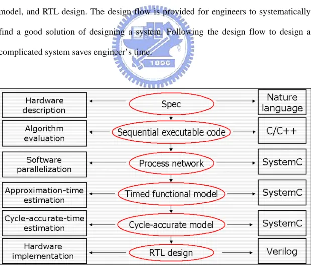
(13) Chapter 2 Preliminary. 2.1 Refinement. As shown in Figure 1, there are five steps in our design flow of refinement: spec, sequential executable code, Process network, timed functional model, cycle-accurate model, and RTL design. The design flow is provided for engineers to systematically find a good solution of designing a system. Following the design flow to design a complicated system saves engineer’s time.. Figure 1 Refinement. 3.

(14) In spec step, nature language is used for hardware description. The step is the starting point of our design flow. Engineers write the need, the inputs and the outputs of the system. Next, engineers use C/C++ language to write the sequential executable code to verify the algorithm in sequential executable code step. After algorithm is verified, the sequential executable code is refined to a process network for parallel computation. Then, the process network is added timing information for estimating time. Finally, engineers write the cycle-accurate model and RTL design of the system.. 2.2 SystemC Features. In our design flow, the process network and the timed functional model of a system are both written by SystemC. In other words, we used SystemC to complete our main work. The reason we use SystemC is that SystemC has many features which are convenient for us to write these. SystemC provides a model of time which is not only easy-to-use but also with high readability [6]. It is convenient for us to use the model of time to add timing information to a model of system. SystemC provides libraries for parallel computation [6]. It is convenient for us to use these libraries to model a system with multi concurrent block. SystemC provides some H/W data types [6]. Instead of spending time to design H/W data types, we use these data types to model hardware’s behavior in the system. SystemC provides mechanism for synchronization [6] [7]. We can use the mechanism to model arbiter’s behavior. Thus, we can study how the system with limited resources works better.. 4.

(15) 2.3 Process Network. Process network is a model of computation and a collection of processes which are connected and communicated over FIFO. Multiple parallel processes can execute simultaneously while using the process network to model a system [5]. We usually use a directed graph notation to represent a process network. In a directed graph notation which is used to represent a process network, nodes are used to represent processes, and edges are used to represent one-way FIFO queues of data. Figure 2 is the typical directed graph notation representing a network with four nodes and three FIFOs. The four nodes are node A, node B, node C and node D. The three FIFOs are FIFO p, FIFO q, and FIFO r. FIFO q connects node A and node B, FIFO r connect node A and node D, and FIFO p connects node B and node C. Node C has an input to the another process network. Node D has an input to another process network, too. Node A has an output to another process network.. Figure 2 A directed graph representing a process network. The set of firing rules be sequential when we use process networks to model a system. Thus, we set our firing rule below. In a directed graph notation which is used to represent a process network, a node is fired just after all its input edges are filled 5.

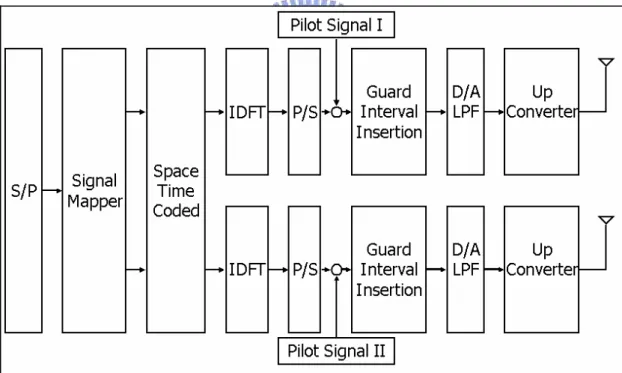
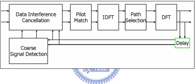
(16) data. It means that a process executes when all its input data arrived.. 2.4 The OFDM System. The OFDM system used by this case study is provided by Meng-Lin Ku and Chia-Chi Huang. Figure 3, Figure 4, and Figure 5 depict the OFDM system blocks. Figure 3 depicts the transmitter architecture part of the system. Figure 4 depicts the receiver architecture part of the system. Figure 5 deeply depicts the Channel Estimation block of the receiver architecture [4].. Figure 3 Transmitter architecture. 6.

(17) Figure 4 Receiver architecture. Figure 5 Channel estimation block. 7.

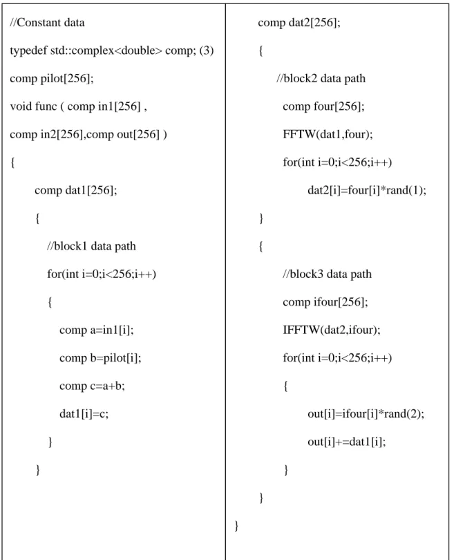
(18) Chapter 3 Our Platform In this work, we apply our design flow we mentioned in 2.1 to the OFDM system we mentioned in 2.4. Accordingly, we refine the model of the OFDM system step by step. We add more information and get more practical result when refining every time. What must be noted is that we focus on how to estimate the execution time of the whole system at this work. Thus, the timing information plays an important role there.. 3.1 Coding. Guideline. of. Sequential. Executable Code. We bring up five coding guidelines which algorithm designers should follow when they writing their C/C++ program. A C/C++ program wrote by these coding guidelines will be easy to be refined into the process network. The detailed description is what follows and the code in Figure 6 illustrates the rules we bring up in this sub-section.. 8.

(19) //Constant data. comp dat2[256];. typedef std::complex<double> comp; (3). {. comp pilot[256];. //block2 data path. void func ( comp in1[256] ,. comp four[256];. comp in2[256],comp out[256] ). FFTW(dat1,four);. {. for(int i=0;i<256;i++) comp dat1[256];. dat2[i]=four[i]*rand(1);. {. } //block1 data path. {. for(int i=0;i<256;i++). //block3 data path. {. comp ifour[256]; comp a=in1[i];. IFFTW(dat2,ifour);. comp b=pilot[i];. for(int i=0;i<256;i++). comp c=a+b;. {. dat1[i]=c;. out[i]=ifour[i]*rand(2);. }. out[i]+=dat1[i];. }. } } }. Figure 6 An example of coding guidelines. We defined that communication variables are variables which are used to exchange data and local variables are variables which are only used in a module there. The first rule we bring up is that the people writing sequential executable code to 9.

(20) verify the algorithm of the system should separate communication variables and local variables. It also implies them should not use global variables. The reason to follow that rule is that it is helpful to find the range, inputs, and outputs of processes. Finding the range, inputs, and outputs of processes in a general C/C++ program is hard. If the communication variables and local variables are separated, the inputs and outputs in a function block are clear. Thus, we can find them easily. Then, we can also infer the code range of the module. The code shown in Figure 6 gives an example of the rule. In the code shown in Figure 6, the local variables are only used for computation in a block, like a, b, and c and the communication variables are used for communication between blocks, like the array “dat1” and the array “dat2”. Take block 1 in the code, the inputs of block 1 are the array “in1” and the array “pilot” and the output of block 1 is the array “dat1” are clear. Finding the inputs and outputs of other blocks is also easy. When refining the sequential code to the process network, verifying the behaviors of sequential code and the process network are the same or not is necessary. If all random functions in the program use the same random sequence, the order of getting random number is changed because the processes in the code may execute parallelly while refining the sequential code to the process network. Therefore, we bring up our second rule, all random functions in the program use different random sequence. If it is followed, we can get the same random number in sequential code and the process network easily. Thus, we could verify the behaviors of sequential code and the process network easily. The statement (1) and statement (2) in the code shown in Figure 6 are the instance of this rule. Complex data is often used in a communication system. Using different data type in a program to model it is trouble to modify the problem. Therefore, we bring up our third rule, using complex data type in C/C++ standard library. Complex data type in 10.

(21) C/C++ standard library should be used to compute complex number because of readability and facilitating modeling data. If we used it, modeling data exchange in different block in the process network may be not annoying and the problem may be easily understand. Otherwise, we may see that different data type used in different module and modeling data exchange spends much time. The statement (3) and these declarations of “comp” in the code instantiate how to follow this rule. The fourth rule we bring up is to consider data grain size which is used in hardware block. While refining the sequential code to the process network, we hope the behavior of the process network is similar to the real system. Thus, we use real data grain size to exchange data. If it is considered when writing sequential code, refining is easier and less time is wasted to complete whole work. In the code shown in Figure 6, the functions compute a symbol of data instead of a packet of data. It accords with the common condition of hardware and sets the example of this rule. The fifth rule we bring up is to keep block operation sequence by topological order. It facilitates modeling inputs and outputs of the whole system. It is important when modeling a system with many blocks. Take the code in Figure 6; the data exchange in the code could use the directed graph to model in Figure 7. Obviously we keep block operation sequence by topological order in the code.. Figure 7 The data exchange of the code example. 11.

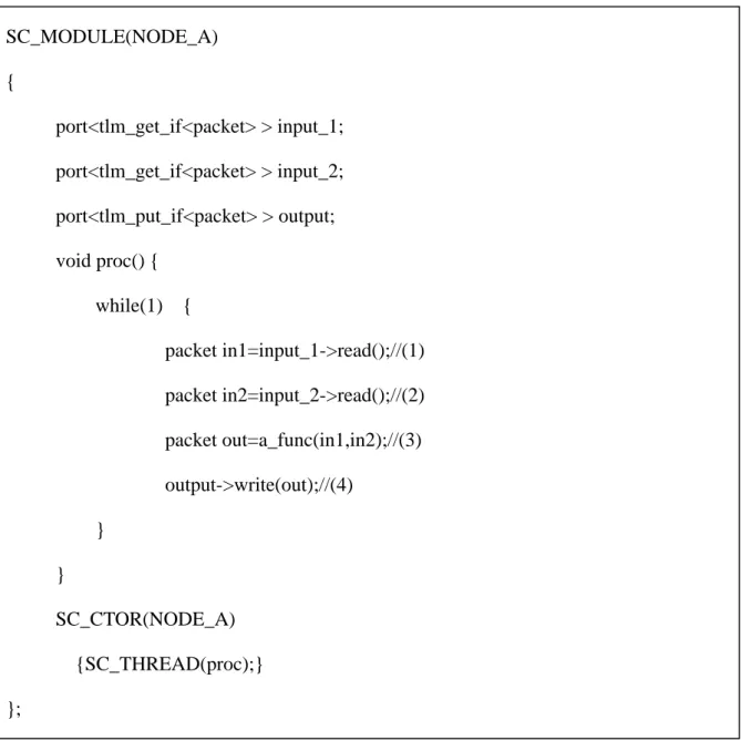
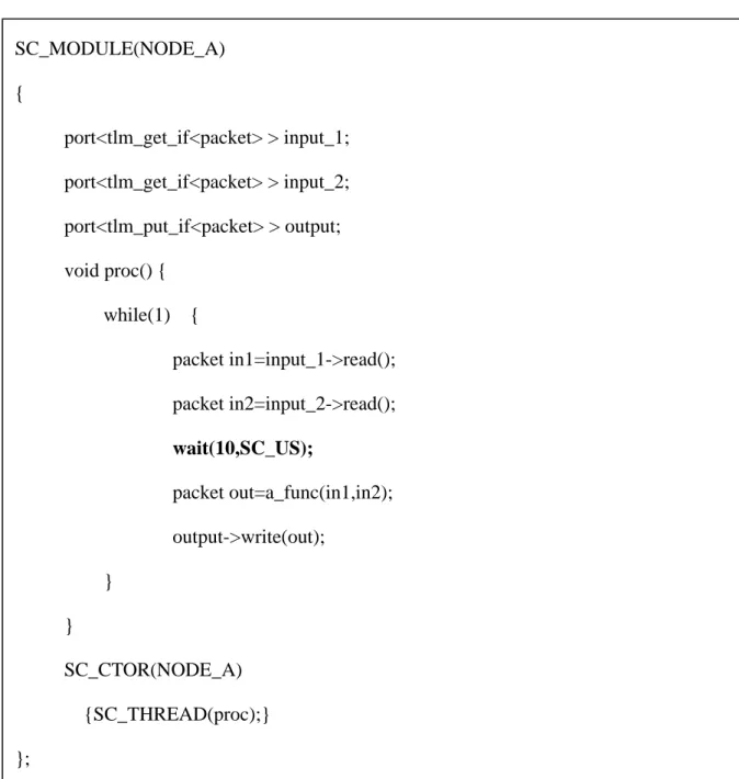
(22) 3.2 A Process Network Model. We establish a process network we mention in 2.3 to model the OFDM system with parallel computation. In this section, we introduce how to establish the process network model. It should be noticed that we use TLM library which is described in [8] to model the system because of convenience. First, we should design how to model a node in a process network by SystemC. The code in Figure 8 is the pattern of the node of the system written in SystemC. In the example of modeling a node, we model the node A in the process network which is mentioned in 3.1. In the object declaration of SystemC in the code, we see the three parts of it the declarations of ports, the body function “proc”, and the object constructor of SystemC. In the function “proc”, the statement (1) is not executed until the input_1, using the get-interface function of TLM library, has data. The statement (2) has same condition, too. That is, they work with blocking read. Thus, our firing rule of process network model is guaranteed. In other words, we guarantee that the process does not execute until all its input queues has data. The part of the object constructor of SystemC puts the function “proc” to an individual thread. And so forth, we can write the SystemC code of other nodes.. 12.

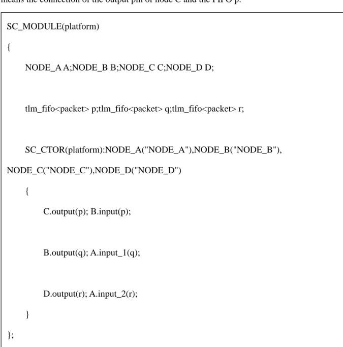
(23) SC_MODULE(NODE_A) { port<tlm_get_if<packet> > input_1; port<tlm_get_if<packet> > input_2; port<tlm_put_if<packet> > output; void proc() { while(1). { packet in1=input_1->read();//(1) packet in2=input_2->read();//(2) packet out=a_func(in1,in2);//(3) output->write(out);//(4). } } SC_CTOR(NODE_A) {SC_THREAD(proc);} }; Figure 8 SystemC code of a node of the process network. The code in Figure 9 is the pattern of the top-view of the system written in SystemC. It illustrates how the connection between nodes and FIFOs are implemented. The process network described by the code in Figure 9 is the same as the process network described by the directed graph in Figure 2. There are the declarations of nodes and FIFOs and an object constructor of SystemC in the object declaration of SystemC in the code. The statements in the object constructor of SystemC describe 13.

(24) how to connect the FIFOs and the node. For example, the statement “C.output(p)” means the connection of the output pin of node C and the FIFO p. SC_MODULE(platform) { NODE_A A;NODE_B B;NODE_C C;NODE_D D;. tlm_fifo<packet> p;tlm_fifo<packet> q;tlm_fifo<packet> r;. SC_CTOR(platform):NODE_A("NODE_A"),NODE_B("NODE_B"), NODE_C("NODE_C"),NODE_D("NODE_D") { C.output(p); B.input(p);. B.output(q); A.input_1(q);. D.output(r); A.input_2(r); } }; Figure 9 The system top-view written in SystemC. Therefore, we use a process network to model the OFDM system in this work. We describe our procedure of making process network model here. First, we divide whole system to processes, according to the original data flow of the system. Then, we use FIFOs to connect these processes. Specially, while modeling the OFDM system using process network, we avoid self-loop when establish process network 14.

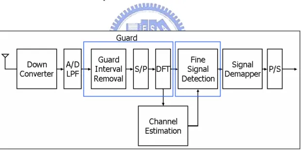
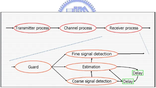
(25) model of a system for being ease to observe the data flow of the system. In this work, we use process network to model an OFDM system. Because we want to observe the operation of the receiver, we divide the receiver to small processes. Figure 10 and Figure 11 depicts how the receiver part of the OFDM system blocks are divided into processes. We will use four processes, “Guard”, “Fine signal Detection” “Estimation”, “Coarse Signal Dectection”, and a delay element and some FIFOs connecting these nodes to model the receiver in the OFDM system. The block “Down Converter” and the block “A/D LPF” are combined to the channel model and the block “Signal Demapper” and the block “P/S” are ignored in the original C code. Thus we ignore these block in our receiver model. We use the method we mentioned in this section to establish the process network in this work.. Figure 10 Receiver architecture divided into processes. 15.

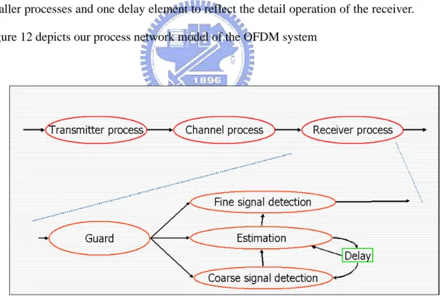
(26) Figure 11 Receiver architecture divided into processes. According to the above-mentioned method, we divide the OFDM system into the process network in Figure 12. We also divide the receiver process into the four smaller processes and one delay element to reflect the detail operation of the receiver. Figure 12 depicts our process network model of the OFDM system. Figure 12 Process network model of the OFDM system. When using the process network to model the OFDM system, the loop including the delay element comes into our notice. The OFDM system uses the channel 16.

(27) estimation value of the last iteration to estimate the channel at this iteration. Estimation and Coarse-signal detection all need the result of Estimation at last iteration. Thus, “Coarse-signal detection” and “Estimation” can not run at the same time because Coarse-signal detection must wait the result Estimation at the same iteration. In consequence, we try to add a delay element after the original delay element as shown in Figure 13 shows. That means the OFDM system uses the channel estimation value of the penultimate iteration. Thus, “Coarse-signal detection” and “Estimation” can run at the same time. It may increase the bit error rate of the OFDM system. However, it also increases the parallelization efficiency. We use the example to prove that changing architecture in the process network level of our design flow is useful.. Figure 13 Process network model of the OFDM system (with two delay element). 3.3 Timed Functional Model. After establishing process network of a system, we add timing information to it 17.

(28) to establish timed functional model of the OFDM system. Hence, we must get timing information for establishing timed functional model. While getting timing information, using hardware or software to implement certain function is must be considered. We get software timing information for modeling a block which is implemented in software and get hardware timing information for modeling a block which is implemented in hardware. Before we get software timing information, we must make the code realistic. Hence, some things must be done before running sequential executable code on instruction set simulator (ISS). For example, two things must be done when establishing timed functional model of the OFDM system. First, fixed-point modification should be considered. If we want to estimate a function which executes on an environment without floating point unit, we should modify the function to a fixed-point function. Second, we should use table-lookup acceleration to accelerate a function which is frequently used because we want to get realistic timing information. Then we run sequential executable code which is modified on ISS and get software timing information. Moreover, we get hardware timing information according to information from the bottom layer or reasonable assumption. Therefore, we add timing information to the process network model of the system. Thus, we get a timed functional model of the system.. 18.

(29) SC_MODULE(NODE_A) { port<tlm_get_if<packet> > input_1; port<tlm_get_if<packet> > input_2; port<tlm_put_if<packet> > output; void proc() { while(1). { packet in1=input_1->read(); packet in2=input_2->read(); wait(10,SC_US); packet out=a_func(in1,in2); output->write(out);. } } SC_CTOR(NODE_A) {SC_THREAD(proc);} }; Figure 14 SystemC code of timed functional model. The code in Figure 14 is the form of a timed functional process model written by SystemC. The difference between the process network model and the timed functional process model is that time timed functional process model is added timing information. The boldface statement in the figure is just the difference in this example. It is a “wait” statement. When the simulator counts the execution time, it waits at the statement for 10 micro-second in this example. Thus, we establish the timed 19.

(30) functional model doesn’t work until all input pins have data, counts its computation time and put its result to their output pins.. 3.4 Resource Management and Scheduling. When the issues of real design are discussed, the problem of limited resource must be paid attention to. Thus, a resource scheduler must exist. In this case study, we must concern memory scheduling and FFT scheduling. When modeling a system without infinite resource, we get the more realistic result from simulation after constructing the mechanism. First of all, we establish a model of resource scheduler to handle resource request in the system model. In the model of resource scheduler, we use mutexes to decide which process gets the resource. A mutex represents a resource available in our scheduler model. When a process requests a resource, the scheduler decides that the process gets resource or not. If there is any resource, the process gets resource; otherwise, the process gets no resource. While the process completes its work about the resource, it usually releases the resource. However, if we would like to transfer the resource and some things sticking the resource to another process, we transfer the resource to the budgeted process. For example, a process may want to transfer the memory and the data in the memory to another process. The transformation is budgeted when designing the system. We will give an example below. In Figure 15, a mutex represent a resource and a man in the figure represents a process. We will use figures of this style to illustrate our mechanism of memory scheduling.. 20.

(31) Figure 15 Motions of resource scheduler I. As shown in Figure 16, when a process requests a memory, the scheduler checks whether there is memory available or not. If there is memory available, the scheduler gives the process a grant to use a memory.. Figure 16 Motions of resource scheduler II. After the process which gets resource in last step completes its work about the resource, it transfers the resource to the budgeted process. This movement transfers 21.

(32) not only the memory but also the data in the memory. Figure 17 depicts it.. Figure 17 Motions of resource scheduler III. As shown in Figure 18, the process with a grant requests another and the scheduler gives a grant to it. Whether a process owns any memory or not, it can always request memory. The scheduler gives it a grant when there is a memory available.. Figure 18 Motions of resource scheduler IV 22.

(33) As shown in Figure 19, the scheduler can handle the requests of two processes at the same time. Besides, if any process requests a memory now, the scheduler does not reply until there is a memory released. While the process gets no response, it stops its work.. Figure 19 Motions of resource scheduler V. 23.

(34) The example in Figure 20 depicts the model of scheduler. The other resources scheduling can completely imitate this form. In the figure, the F1 block and the F2 block are general processes and the FFT1 block and the FFT2 block represent the processes with FFT functions. We assume there is only a FFT block in hardware in the example. First, FFT1 request the FFT block in hardware and get grant. Second, FFT2 request the FFT block in hardware, gets no grant, and wait that until there is a FFT block in hardware available in the system. Third, the FFT1 complete its work about FFT function and release the FFT block in hardware and FFT2 gets the grant and starts their work.. Figure 20 The model of resource scheduling. 24.

(35) SC_MODULE(sched) { void Request() { push job to queue; wait grant event;} void Release(){ signal release event; } void Proc(){ while(1){ wait job; find next job; signal grant event; wait release event; } } SC_CTOR(sched) {SC_THREAD(proc);} }. Figure 21 The pseudo-code of resource scheduler. Figure 21 shows the code pattern of a scheduler written in SystemC. The SC_MODULE in Figure 21 has three sub-functions Request, Release, and Proc. The 25.

(36) object constructor of SystemC describes that Proc is put in an independent thread. Then, the Proc finds next job to execute, signal grant event and wait release event. When a process wants to request a resource, it calls the request function. The request function pushes a job to queue and wait for grant event. Then, when it completes its work about the resource, it calls the release function. Therefore, we use the mechanism above-mentioned to model our scheduler.. 26.

(37) The code in Figure 22 is the pattern of a process connecting to a scheduler written in SystemC. The process requests the hardware resource, waits the grant, computes its function, and releases the hardware resource.. SC_MODULE(estimation) { port<tlm_get_if<packet> > input; port<tlm_put_if<packet> > output; port<sched> fft_sched; void proc() { while(1). { packet in=input->read(); fft_sched->request();//(1) wait(10,SC_US); packet out=fft_func(in); fft_sched->release();//(2) output->write(out); }. } SC_CTOR(estimation) {SC_THREAD(proc);} };. Figure 22 SystemC code of timed functional model with resource scheduling. About the OFDM system used at this case study, there are two aspects we concern about scheduling: FFT scheduling and memory scheduling. We will make a 27.

(38) detailed description with two figures, Figure 23 and Figure 24, below. Figure 23 depicts the mechanism’s operation of memory scheduling at our case study. We describe how it works in an iteration below. There are several steps in an iteration. At first, we always give the delay element a grant of one unit memory, and the first arrow points out the transaction. When the whole system starts, the process “Guard” request one unit memory. The second arrow points out this transaction. It starts to computer its result when getting the grant of one unit memory. After finishing its work, it transfers its result and the grant of the memory which it got to “Coarse-signal detection”, “Estimation”, and “Fine signal detection”. Then, the process “Coarse-signal detection” starts to work and request another unit memory to store data, and the third arrow points out the transaction. There the process “Coarse signal detection” can not use the memory which the process “Guard” to store its output because the result of the process “Guard” is used by the two other processes, the process “Estimation” and the process “Fine signal detection”. Then, the result of “Coarse signal detection” and that memory are transferred to the process “Estimation” after “Coarse signal detection” finishes its work. Thus the process “Estimation” uses the memory got by “Guard” and “Coarse-signal detection” to finish its work. “Fine signal detection” does too. “Estimation” transfer its data and the memory got from “Coarse signal detection” to “Fine signal detection”. Finally, the fourth arrow points out that the process “Fine signal detection” finish its work and release the two memories got form the process “Estimation”.. 28.

(39) Figure 23 OFDM memory scheduling. Figure 24 depicts the mechanism’s operation of FFT scheduling at our case study. We connect the process having FFT function to FFT scheduler. While these processes need a FFT block in hardware, they send a request to FFT scheduler. If they get grants, they compute their FFT function. If they get no grants, they wait until the scheduler gives them grants. After they finish their work about FFT function, they release the FFT block in hardware to the FFT scheduler. Because the FFT block in hardware does not need transfer data, the mechanism of FFT scheduling is simpler than memory scheduling.. 29.

(40) Figure 24 OFDM FFT scheduling. When observing the operation of the timed functional model with a scheduler, we see that the process “Guard” gets memory too often. It makes the system work inefficiently. We think that setting the order of memory grant at this case study may make the system more efficient. We will see the effect at this case study in Chapter 4. We describe how to set the order below. As shown in Figure 25, the delay element always gets a unit of memory; the process “Guard” and the process “Coarse signal detection” get one unit of memory and another unit of memory in an iteration respectively. In the same iteration, the process “Guard” sends a request to the memory scheduler before the process “Coarse signal detection” sends a request to the memory scheduler. Thus, we set that the process “Guard” does not gets grant before the process “Coarse signal detection” gets in the last iteration. We will see the effect at this case study in Chapter 4.. 30.

(41) Figure 25 OFDM memory static scheduling. 31.

(42) Chapter 4 Experimental Results. 4.1 Experimental Information. In this chapter, we introduce some experiments with different hardware architecture and different scheduling strategy on our platform. These experiments confirm practicability of our platform. As we said earlier, we must get hardware timing or make reasonable assumptions make timed functional model. At this case study, FFT architecture and the latency of matrix operation are the factors. Table 1 shows that how we make the assumption about the two factors. Besides, all of our experiments compute 30000 symbols.. Item. Clock. Complex number adder timing. 100MHz. Complex number multiplier timing. 100MHz. Butterfly processing element timing. 100MHz. Table 1 Experimental fundamental assumptions of timing. 32.

(43) We base on these assumptions to decide the timing of modules in the system. Then we make simulation of systems with different scheduling strategy and different hardware architecture to verify the effect of static scheduling, adding delay element to increase parallelism and different FFT architectures. These experiments also verify that platform based design is helpful for design space exploration. The experimental results are introduced in 4.2.. 33.

(44) 4.2 Experimental Results. 4.2.1 Experiment Experiment I is our general case. In other words, the result is our standard to let us understand the effect of different scheduling strategy and different hardware architecture. The hardware architecture of system in experiment I is shown in Table 2.. Item. Architecture. Memory. 2048 bytes, unlimited memory bandwidth. FFT. Memory based, radix-4. Delay element. One. Static scheduling. none. Table 2 Experimental assumptions of architecture in experiment I. Figure 26 shows the result of experiment I.. OFDM execution time (ms). 350 300. FFT. 250 1. 200. 2 150. 3. 100 50 0 4. 5. 6 Memory. Figure 26 OFDM execution time of experiment I (ms) 34. 7.

(45) In the figure, we see that using more than two units of FFTs hardware or more than six units of memories does not help decrease the execution time and the system in the condition gets no result with less than four units of memories. In 3.2, we supposed that if a delay element is added to the system, the system may be more efficient than the original system. In experiment II, we verify whether the strategy is valid or not. The hardware architecture of system in experiment II is shown in Table 3.. Item. Architecture. Memory. 2048 bytes, unlimited memory bandwidth. FFT. Memory based, radix-4. Delay element. Two. Static scheduling. none. Table 3 Experimental assumptions of architecture in experiment II. Figure 27 shows the result of experiment II.. 35.

(46) OFDM execution time (ms). 350 300. FFT. 250 1. 200. 2. 150. 3. 100 50 0 5. 6. 7. 8. Memory. Figure 27 OFDM execution time of experiment II (ms). In the figure, we see that using more than two units of FFTs hardware or more than seven units of memories does not help decrease the execution time and the system in the condition gets no result with less than five units of memories. Experiment III We supposed that our mechanism of static scheduling decreases the need of resource in 3.4. In experiment III, we verify the mechanism we suggested is efferent or not. The hardware architecture of system in experiment III is shown in Table 4.. Item. Architecture. Memory. 2048 bytes, unlimited memory bandwidth. FFT. Memory based, radix-4. Delay element. One. Static scheduling. Set the order of memory grant. Table 4 Experimental assumptions of architecture in experiment III. 36.

(47) Figure 27 shows the result of experiment III.. OFDM execution time (ms). 350 300 FFT. 250. 1 2 3. 200 150 100 50 0 3. 4. 5. 6. Memory. Figure 28 OFDM execution time of experiment III (ms). In the figure, we see that using more than two units of FFTs hardware or more than five units of memories does not help decrease the execution time and the system in the condition gets no result with less than three units of memories. We use the strategy suggested in 3.2 and our mechanism of static scheduling suggested in 3.4 in Experiment IV at the same time. Table 5 depicts the hardware architecture of system in experiment IV.. Item. Architecture. Memory. 2048 bytes, unlimited memory bandwidth. FFT. Memory based, radix-4. Delay element. Two. Static scheduling. Set the order of memory grant. Table 5 Experimental assumptions of architecture in experiment IV 37.

(48) Figure 28 shows the result of experiment IV. OFDM execution time (ms). 350 300 FFT. 250. 1. 200. 2 150. 3. 100 50 0 4. 5. 6. 7. Memory. Figure 29 OFDM execution time of experiment IV (ms). In the figure, we see that using more than two units of FFTs hardware or more than six units of memories does not help decrease the execution time and the system in the condition gets no result with less than four units of memories. The convenience of changing architecture in a system model is one main advantage of platform design. It allows us try different architectures in a system to find the best configuration of hardware. Experiment V just exhibits the convenience. Table 6 depicts the hardware architecture of system in experiment V. We change the FFT architecture in the system.. 38.

(49) Item. Architecture. Memory. 2048 bytes, unlimited memory bandwidth. FFT. Memory based, radix-4. Delay element. One. Static scheduling. None. Table 6 Experimental assumptions of architecture in experiment V. Figure 30 shows the result of experiment V.. OFDM execution time (ms). 450 400 350. FFT. 300. 1. 250. 2. 200. 3. 150 100 50 0 4. 5. 6. 7. Memory. Figure 30 OFDM execution time of experiment V (ms). In the figure, we see that using more than two units of FFTs hardware or more than six units of memories does not help decrease the execution time and the system in the condition gets no result with less than four units of memories. It also shows the effect of FFT architecture the system in the condition gets no result with less than four units of memories.. 39.

(50) 4.2.2 Performance Analysis. OFDM execution time (ms) # of memories # of FFTs Ex. 1. Ex. 2. Ex. 3. Ex. 4. Ex. 5. 3. 4. 5. 6. 7. 8. 1. x. x. 322. X. X. 2. x. x. 300. x. X. 1. 292. x. 292. 322. 384. 2. 276. x. 276. 299. 322. 1. 292. 292. 230. 292. 384. 2. 276. 276. 215. 277. 322. 1. 230. 290. 230. 172. 323. 2. 215. 274. 215. 156. 261. 1. 230. 172. 230. 172. 323. 2. 215. 156. 215. 156. 261. 1. 230. 172. 230. 172. 323. 2. 215. 156. 215. 156. 261. Table 7 Performance analysis. Table 7 shows all of our experimental result expect cases using three units FFT architecture. We ignore cases using three units of FFT hardware there because the results of these cases are the same as cases using two units of FFT hardware and we show these things above. In the table we see some interesting thins we mention below. In experiment II, we add a delay element to increase parallelism. The strategy spends more memory. However, it decreases the execution time when the system has 40.

(51) sufficient memory. Thus, it gets good performance with these cases using seven and eight units of memories. In experiment III, we use static scheduling to make good use of memories. Thus, it gets good performance with these cases using five and three units of memories. In experiment IV, we use static scheduling and add a delay element at the same time. It gets good performance with these cases using six units of memories. Therefore, we see that design space exploration at electric system level is useful. It helps us choice different architectures at different condition. For example, at this case study, we can decide which architecture should be used basing on these experimental results, like deciding to use static scheduling and add no delay element when having only three units of memories to use etc. Besides, we also can see the effect of FFT architecture in experimental results. It should notice that the process may transfers memories to another process instead of releasing every condition. Thus, some cases without enough can not get results.. 41.

(52) Chapter 5 Conclusion and Future Work In this work, we apply a top-down design methodology to an OFDM design. By incorporating the process network model, the timed functional model, systems with different configurations can be simulated in a short time. Some important parameters are then extracted from the simulation result and the performance of the system can be assessed before the system is implemented. Concretely speaking, we establish a framework with process network model, timed functional model, and resource scheduling for design space exploration and design modeling. Performances of systems with different configurations can be examined. Also, we try to use our framework to verify our static scheduling mechanism and our idea to increase parallelism. The experimental results show that our platform is practical.. 42.

(53) Reference [1] A. Sangiovanni-Vincentelli, “Defining platform-based design,” in EEDesign of EETimes, 2002 [2] J. Henkel, “Closing the SoC design gap,” in Computer, Sept. 2003, Volume 36, Issue 9, pages 119 – 121 [3] F. Balarin, Y. Watanabe, H. Hsieh, L. Lavagno, C. Passerone, A. Sangiovanni-Vincentelli, “Metropolis: An Integrated Electronic System Design Environment,” in IEEE Computer, April 2003, p 45-52. [4] M.-L. Ku and C.-C. Huang, “A complementary code pilot-based transmitter diversity technique for OFDM systems,” in IEEE Transactions on Wireless Communications, March 2006, Volume 5, Issue 3, pages 504 – 508 [5] G. Kahn, “The semantics of a simple language for parallel programming," in Proceedings of the IFIP Congress, 1974. [6] SystemC 2.0.1 Language Reference Manual, 2003. Available from the Open SystemC Initiative (OSCI) http://www.systemc.org. [7] Sudeep Pasricha, "Transaction level modelling of soc with SystemC 2.0,” In Synopsys User Group Conference, 2002. [8] A. Rose, S. Swan, J. Pierce, and J. Fernandez. “Transaction Level Modeling in SystemC,” OSCI TLM Working Group, 2005.. 43.

(54) VITA Guan-Hao Chen was born in Hualien, Taiwan on April 6, 1982. He received the B.S. degree in Electronics Engineering from National Chiao Tung University in June 2004 and entered the Institute of Electronics, National Chiao Tung University in September 2004. His research interests include electronic design automation (EDA) and VLSI design. He received the M.S. degree from National Chiao Tung University in August 2006.. 44.

(55)

電子系統層級上的設計方法 － 以正交多頻多工系統為例

電子系統層級上的設計方法－以正交多頻多工系統為例