Application of the sliding mode fuzzy controller to the guidance and control of an autonomous underwater vehicle

APPLICATION OF THE SLIDING MODE FUZZY CONTROLLER

TO THE GUIDANCE AND CONTROL OF AN AUTONOMOUS

UNDERWATER VEHICLE

F.C. Chiu, J. Guo, C.C. Huang, W.C. Tsai

Dept. of Naval Architecture and Ocean Engineering

National Taiwan University, Taipei, Taiwan, R.O.C.

E-mail: [email protected]

Abstract

-

This paper show that a sliding mode fuzzy controller is quite satisfactory for the control and line of sight tracking performance of an autonomous underwater vehicle developed at this institution. The design method of the sliding mode fuzzy controller allows a systematical method to construct a set of membership functions, called shrinking-span membership functions and dilating-span membership functions, for a specific linguistic variable. This gives the controller design more convenience to deal with non-linearities of the vehicle dynamics and the environmental disturbances. Effects of using different design parameters are evaluated through experiments.

I . INTRODUCTION

Control problems related to AUVs presents several difficulties, due to their non-linear dynamics, the presence of disturbance, and the observation noises. In recent years, an increasing amount of attention has been devoted to the exploration of oceans and the utilization of oceanic resources located in shallow, confined water areas. In such regions, shallow water phenomena from the interaction of wave dynamics, tidal currents, coastal currents, ocean currents, and artificial objects result in a complex environment for the operation of unmanned underwater vehicles. Therefore, control of AUVs to perform satisfactory trajectory tracking behavior in shallow waters is still a challenging problem.

In this article, we show an efficient controller to control the direction of a flat, streamlined AUV which is developed currently underway to test AUV related technologies such as design capabilities, guidance, navigation, control, underwater imaging, and communications. Missions of the AUV Hai-Min (AUV- HM1) are designated for area search and survey in shallow water. Typical searchhurvey scenario in large area requires route stability and good turning performance in the horizontal plane of motion. Therefore, directional control is

a basic feature for this AUV motion control system. Fuzzy logic controllers have been recognized as effective robust controllers for a variety of applications. One of the advantages in using fuzzy logic to design a controller is that the dynamics of the controlled system need not be completely known. However, the linguistic expression of the fuzzy controller makes it difficult to guarantee the stability and robustness of the control system. The sliding mode control [ 11 can also be applied well in the presence

of

model uncertainties, parameter variations, and disturbances. The disadvantage of the sliding mode control is the chattering behavior at the sliding surface. Designing a fuzzy logic controller based on the sliding mode theory assures the performance and stability, it also reduces the number of fuzzy rules. Furthermore, fuzzy partition of the manipulated variables avoids chattering problem of the sliding mode control method [2]. The ‘fuzzy sliding mode controller’ is therefore adopted in this paper as the basic controller structure to be investigated.

In recent years, several control strategies based upon fuzzy logic or sliding mode have been published for the application in the motion control of underwater vehicles. Please refer to [3,4,5].

11. VEHICLE

MODELING

A two-degree-of-freedom vehicle model is used since the motion is restricted to the horizontal plane. The model including drag, added mass, and thrust moment for yaw motion is

I .i.

+

br

I

r

I

= U ₍₁₎

where I is the vehicle’s mass moment of inertia in addition to the added inertia of the body about the body-fixed z-axis. r is the body-fixed rate for heading direction. b is the square-law damping coefficient. U is the moment generated

by commanding different thrust force on the left and right thrusters.

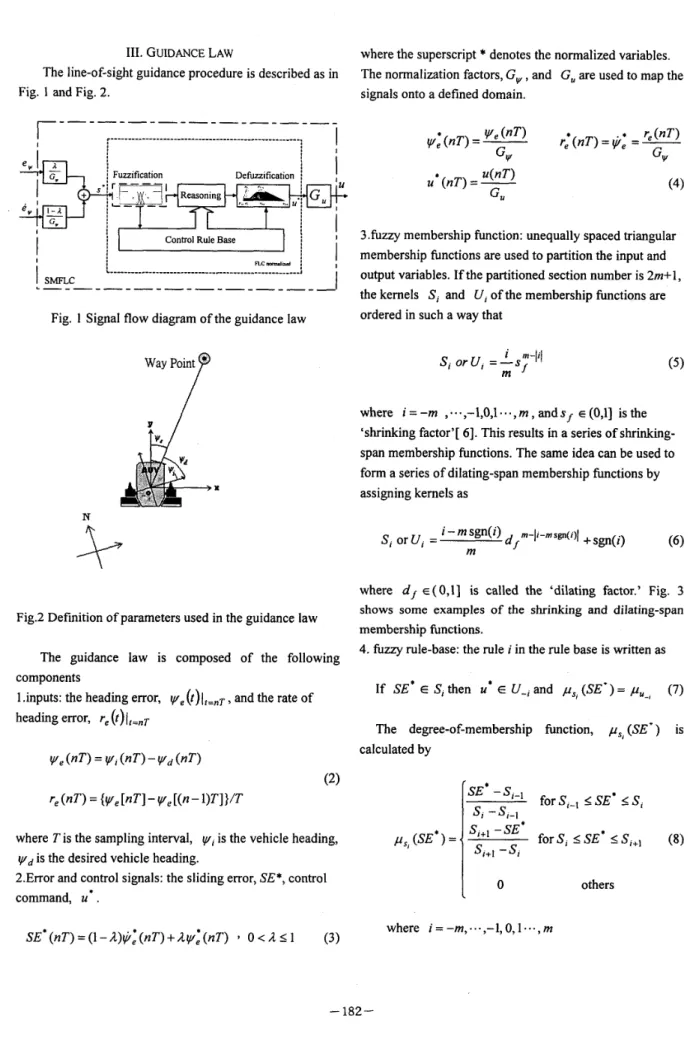
111. GUIDANCE LAW

The line-of-sight guidance procedure is described as in Fig. 1 and Fig. 2.

Fuvification Defuaification !

Fig. 1 Signal flow diagram of the guidance law

N

Way Point

*

P

X

where the superscript * denotes the normalized variables. The normalization factors, G, , and G, are used to map the signals onto a defined domain.

(4)

3 .fuzzy membership function: unequally spaced triangular membership functions are used to partition the input and output variables. If the partitioned section number is 2m+l, the kernels S, and U , of the membership functions are ordered in such a way that

i m+I

m

Si orU, =-sf _{( 5 )}

where i = - m , . . a , - l,O,l...,m,andsf ~ ( 0 , 1 ] isthe

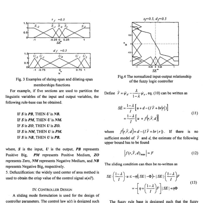
‘shrinking factor’[ 61. This results in a series of shrinking- span membership functions. The same idea can be used to form a series of dilating-span membership functions by assigning kernels as

where

df

E (0,1] is called the ‘dilating factor.’ Fig. 3 shows some examples of the shrinking and dilating-span membership functions.

4. fuzzy rule-base: the rule i in the rule base is written as If SE* E Sf then U * E U-, and ,us, (SE‘) = p,-, (7) The degree-of-membership function, ,us, ( S E - ) is

Fig.2 Definition

of

parameters used in the guidance law The guidance law is composed of the following components

1 .inputs: the heading error, ~ / ~ ( t ) ( ~ , , ~ , and the rate of heading error, re (t)IlznT

calculated by

Ye ( n T ) = V I ( n r ) - Yd ( n T )

SE* -S,-l

for

s,-,

s

SE*

s

S ,

SI -s1-1

where Tis the sampling interval, Y , is the vehicle heading, V / d is the desired vehicle heading.

2.Error and control signals: the sliding error, SE*, control command, U * .

Pcs, (SE* ) = for S, 5 SE’ 2

s,+~

₍₈₎

others

SE* (nT) = (1 -A)& (nT)

+

AY: ( n T ) ’ 0 < A I 1 (3) where i = -m,

.

,-1, O,l--. , m

~ ~ 0 . 5 , d f 0 . 5 J -1 -0.25 0 0.25 1

Sd

d r =0.5 -1 -0.75 0.75 1 U

Fig. 3 Examples of shring-span and dilating-span memberships functions 1 0.5 *3 O -0 5 1 1 -0.25 0 0.25 1 SE*

Fig.4 The normalized input-output relationship of the fuzzy logic controller

For example, if five sections are used to partition the linguistic variables of the input and output variables, the

a .

Define

? = $ i d

--ye,eq.(lO)canbewrittenas 1 - a

following rule-base can be obtained. IF S is PB, THEN U is NB. IF

S

is PM, THEN

U

is NM. IF S is ZO, THEN U is 20. IF S is NM, THEN U is PM. IF S is NB, THEN U is PB.

.

1 - a SE = -[U

+

d

-

( I

?

+brlrl)] (11) I I =

I-il

[ U

+

f ( r ,

?,

d)] where f ( r ,

?,

d ) =

d - ( I

?

+

br

I

r

I)

.

If there is no sufficient model of

?

and d, the estimate of the following upper bound has to be found

where, S is the input, U is the output, PB represents Positive Big, PM represents Positive Medium, ZO represents Zero, NM represents Negative Medium, and NB

represents Negative Big, respectively. The sliding condition can then be re-written as 5. Dehzzification: the widely used center of area method

is

used to obtain the crisp value of the control signal u(n2'). SE

.(

!+).U 2 -qo SE

1 -m)- I

SE

1 .

-

( 7 ) F (13) IV. CONTROLLER DESIGN = - [ q + ( Y ) F ] l S E l + @

A sliding mode formulation is used for the design of controller parameters. The control law u(t) is designed such that the system trajectories are ultimately bounded under the region B =

{ r ,

I SE(r,

t ) I 0} ; 0 > 0

.

The goal can be achieved by satisfying the following sliding condition

The fUzzy rule base is designed such that the fuzzy control has a similar form as the sliding mode Controller with a boundary layer

(14)

SE

m

U = -K(SE,

a).

sat(-)

outside the region B [ 13

The dynamics of the sliding error SE is determined from eq.(3), in which, the acceleration of yawing angle can be

obtained from eq. (l), thus and K(SE, A)?

0

.

When

I

SE

I?

0 , the sliding condition holds, therefore, by replacing U in eq. (13), we obtain a

U * < - ( 3 ) { [ 7 7 + ( 7 ) F ] - 3 } if SE*

> O

(15) When

1

SE

1

<

C P ,

the tuning of the transfer function from SE* to U* can be performed by arranging the shape of the input and output membership functions. According to the design principles of sliding mode controllers, the ‘balance condition’ [ 11 inside this region should be fulfilled to avoid high-frequency unmodeled dynamics. In other words, the design principle of the slope of the transfer function in the vicinity of the origin is

The slope at the origin can be designed by choosing proper shrinking and dilating factors. If we approximate the shape of the transfer function piece-wise linearly, discontinuous points of the piece-wise linear function occur at the kernel values of input triangular membership functions[2]. Therefore, a reasonable selection of the parameter

CP

will be the first kernel (i=land -1, eq. (5) and

(6)) of the input membership function. For example, if an

input shrinking factor 0.5 is used, then @ = U , = 0.25G,

.

Fig.5 illustrates contours of slope at the origin of the transfer function.

2 4 6 8 1 8 6 4 2

shrinking factor Input dilating factor

Fig. 5

I

U * / S E *

I

at the origin in terms of the paring of input-

output shrinking and dilating factors

From eq.( 1 9 , the parameter G, can be determined by letting

SE*

+.CO, U * +.-I

In order to design the fuzzy controller, from eq. (15) and eq. (16), design parameters, 7, G, , G, , and il are

needed. Parameter 77 is inversely proportional to the time required to reach the region B from an outside initial condition. Parameter G, and G, affect the slope of the controller’s transfer function, and therefore determine the behavior of the system in the vicinity of the origin. Higher the value ofG, (or 77 ), lower the value ofG, result in a faster transient responses. Furthermore, the value of

x-

specifies the rate of convergence to the sliding surface. In [I], a possible choice for the value of

x-

A is suggested as one fifth of the sampling frequency.

V. EXPERIMENTS

Tank tests and sea trials were conducted to investigate effects of the design parameters. The testing tank is 120-m (L) x8-m (W) x4-m (D). The testbed vehicle AUV-HM1 shown in Fig.6 has dimension of 2-m (L)xl-m (W)x0.6-m (D). It is equipped with a 300 kHz Doppler Velocity Log and a fiber-optics gyro as navigation sensors. The sea trial area has a water depth of 60 to 80 meters. The vehicle is submerged at depth of 2 meters below surface.

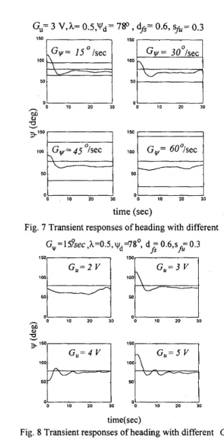
1. Effects of G, , G, , and

R

: directional change command is given while the vehicle is moving with a forward velocity of 0 . 8 d s e c in a water tank. The effects of G,,

G,

,

il on transient responses are illustrated in Fig.7 to Fig

9. It is shown that due to the uncertainties in the process, to achieve precise tracking is possible using the fuzzy sliding mode controller. However, considering the task goal, it is necessary to find a tradeoff between the tracking precision and the control bandwidth.

During sea trials, we commanded the vehicle to follow

a series of waypoint circles of origin [xkd , y k d ] , and radius

go

.

If the present vehicle position [x,

,

y, ]satisfies the following condition

the guidance algorithm triggers the selection of the next waypoint. The magnitude of uncertainty bound F is affected by the waypoint selection, the magnitude of ocean currents, and the vehicle’s dynamics.

150 I

5 . P

Vc= 0.43 m/s, D c= 101' 0 10 20 30 0 10 20 30 h

2

'0, 2c tc- time (sec)

Fig. 7 Transient responses of heading with different G, Gw=15~sec,h=0.5,~d=780, d = 0.6,s =0.3

fs

fu - _current 1501

,

1501 I lIib-Gu=

1

50 0 0 10 20 30 0 10 20 30

2

s

3:::---4

:fq

50 0 0 10 20 30 0 10 20 30 time(sec)

Fig. 8 Transient responses of heading with different Gu

50

'

0 10 20 30 10 20 30 time (sec)

Fig. 9 Transient responses of heading with different A

2. The effect o f t , : Fig. 10 shows the results of straight- line path tracking under two different

4,

s.

3. The effect of F : square-route path tracking results are shown in Fig. 11. Their corresponding F can be calculated from experimental data. Noted that at the path transition from one side of the square path to another side, the uncertainty bound F underwent a large variation. At transition periods, there are large distances between the state and the sliding surface, the unmodeled dynamics can not change the sign of the control input. Therefore, we evaluated this bound only in the vicinity of the origin of the sliding error. To calculate the magnitude of

E

the following parameter values were used: 1=24.13 Kgr .m.sec2, b=32.50 Kgr .m.sec2

,I

d,,

I

=1.02 Kgf .m .The moment of inertia 1, including added moment of inertia, was measured using a Planar Motion Mechanism[7], the damping coefficient b was derived from yaw step responses' data, and the cross flow moment at the current velocity 0.5 d s e c , was measure by tank tests. Fig.12 shows that

F

= 4.5Kg m

,

which was calculated for the path segment from point 1 to point 2 of the lower plot of Fig.11. The value of Gu is therefore selected to be 9.5

Kg

.

m

, which, after a unit conversion from torque to command voltage, is 5

V.

Fig.13 illustrates the transfer hnction of one of the sliding mode controllers used in our sea trials.

&=.7 m,s/-=0.3, ~ " = O . ~ , ~ = O . ~ , G ~ ~ ~ ~ S ~ C , G I F S V

s

'1

I"""

current

X(m)

Fig. 10 Straight-line path tracking under the influences of currents and the radius of the waypoint circle.

E+= 5 m, ys 4.3, d f 3 . 9 , h =0.7,G, =lSo~ec,G, =5 V

Y

h E

s

.lO 0 10 m X(m)

Fig. 11 Square routes path tracking under the influences of currents and the radius of the waypoint circle.

time(sec.)

Fig. 12 The uncertaintyf; and its bound F, calculated from test data for the path segment from point 1 to 2 in Fig 11.

VI. CONCLUSION

We showed that a fizzy sliding mode controller could be used for an AUV in shallow water line-of-sight guidance in the horizontal plane. The fuzzy logic controller is designed based on the principle of fizzy sliding mode. Design parameters were specified, and the effects of them were tested by experiments.

* . .

. . .

-0.5- * . I . . I , . . I . . I l l 1 -0.15 0 0.15 1

SE

*

Fig. 13 Transfer function of the fuzzy sliding mode controller and its stability and robustness bound for the sea

test case shown in the upper plot of Fig. 11.

ACKNOWLEDGEMENT

This research is supported by the National Science Council of R.O.C., under project number NSC88-2611-

REFERENCES

E002-020.

1. J. J. E. Slotine, W. Li, Applied Nonlinear Control, Prentice-Hall, 199 1.

2. R. Palm, “Robust control by fizzy sliding mode,”

Automatica, Vo1.30, No. 9, pp. 1429-1437, 1994. 3. P. A. DeBitetto, “Fuzzy logic for depth control of

unmanned undersea vehicles,” IEEE Journal of Oceanic

Engineering, Vol. 20, No.3, pp. 242-248, 1995. 4. J. P. V. S. Cunha, R. R. Costa, L. Hsu, “Design of a high

performance variable structure control of ROV’s,”

IEEE Journal of Oceanic Engineering, Vol. 20, No.1, 5 . A. J. Healey, D. Lienard, “Multivariable sliding mode control for autonomous diving and steering of unmanned underwater vehicles,” IEEE Journal of

Oceanic Engineering, Vol. 18, No.3, pp. 327-339, 1993. 6 . C.-L. Chen, C.-T. Hsieh, “User-friendly design method for fizzy logic controller,” IEE Proc. -Control Theory

7. F. C. Chiu, J. Guo, C. C. Huang, J.P. Wang, “On the linear hydrodynamic forces and the maneuverability of an unmanned untethered submersible with streamlined body (2”d report: lateral motion),” (in Japanese), No. 182, Journal of the Japanese Society of Naval Architecture, pp. 15 1

-

159, 1997.

pp. 42-55, 1995.

Appl., Vol. 143, NO. 4, pp. 358-366, 1996.