Adaptive Kernel Principal Component Analysis (KPCA) for Monitoring Small
Disturbances of Nonlinear Processes
Chun-Yuan Cheng*
Department of Industrial Engineering and Management, Chaoyang UniVersity of Technology 168 Jifong E. Road, Wufong Township, Taichung County, 41349, Taiwan
Chun-Chin Hsu
Department of Industrial Engineering and Management, Chaoyang UniVersity of Technology 168 Jifong E. Road, Wufong Township, Taichung County, 41349, Taiwan
Mu-Chen Chen
Institute of Traffic and Transportation, National Chiao Tung UniVersity 114 Chung Hsiao W. Rd., Sec. 1, Taipei, 10012, Taiwan
The Tennessee Eastman (TE) process, created by Eastman Chemical Company, is a complex nonlinear process. Many previous studies focus on the detectability of monitoring a multivariate process by using TE process as an example. Principal component analysis (PCA) is a widely used dimension-reduction tool for monitoring multivariate linear process. Recently, the kernel principal component analysis (KPCA) has emerged as an effective method to tackling the problem of nonlinear data. Nevertheless, the conventional KPCA used the sum of squares of latest observations as the monitoring statistics and hence failed to detect small disturbance of the process. To enhance the detectability of the based monitoring method, an adaptive KPCA-based monitoring statistic is proposed in this paper. The basic idea of the proposed method is first adopting the multivariate exponentially moving average to predict the process mean shifts and then combining the estimated mean shifts with the extracted components by KPCA to construct the adaptive monitoring statistic. The efficiency of the proposed monitoring scheme is implemented in a simulated nonlinear system and in the TE process. The experimental results indicate that the proposed method outperforms the traditional PCA and KPCA monitoring schemes.
1. Introduction
Quality is an important issue for modern competitive indus-tries. The statistical process control (SPC) indicates a set of well-recognized techniques for univariate process monitoring, which include Shewhart charts, exponentially weighted moving average (EWMA) and Cumulative Sum (CUSUM) charts. However, hundreds or thousands of variables can be online recorded per day due to the rapid advancement of information technology. Therefore, developing multivariate statistical process monitoring (MSPM) schemes for detecting faults of multivariate processes becomes critical.
The principal component analysis (PCA) can project high dimensional data onto a lower dimensional space that contains the most variance of original data, and hence it has become a popular preprocessing tool for MSPM. Jackson1 initially developed a T2control chart for the PCA-based monitoring method. Further, Jackson and Mudholkar2introduced a residual analysis for based MSPM. After the initial wok of PCA-based MSPM, Ku et al.3 developed a dynamic PCA (called DPCA) by adding time-lagged variables into the data matrix in order to capture the process dynamic characteristics. After that, Tsung4 used DPCA for monitoring and diagnosis of the automatic controlled processes. Since PCA is sensitive to outliers, Hubert et al.5,6 proposed the adjusted outlyingness measurement for filtering outliers before performing the PCA algorithm and named this algorithm as robust PCA (ROBPCA).
Several related works of PCA-based MSPM can refer to Nomikos and MacGregor,7,8 Bakshi,9 Li et al.,10 Shi and Tsung,11and Cho et al.12
As mentioned above, the PCA has been successfully applied for monitoring a multivariate process. However, PCA can only deal with the linear system. To handle the problem of nonlinear process data, several nonlinear PCA approaches have been developed. Kramer13presented a nonlinear PCA method based on the autoassociative neural networks. However, the proposed network is difficult and time-consuming in sample data training because the network consists of five layers which are the input, mapping, bottleneck, demapping, and output layers. Dong and McA-voy14further combined a principal curve and a neural network to formulate a nonlinear version of PCA. In their work, the associated scores and the corrected data points for training samples are obtained by the principal curve method (Hastie and Stuetzle15). The neural network is then used to map the original data into the corresponding scores and to map these scores into the underlying variables. Alternative works in this area are summarized as follows. Tan and Mavrovouni-otis16 suggested a nonlinear PCA method based on input-training neural network; Jia et al.17further combined linear PCA and input-training neural network to separately deal with linear and nonlinear data correlations.
According to the above literatures, most nonlinear PCA methods are based on neural networks. It means that the resulting network training includes the solving of a hard nonlinear optimization problem which has the possibility of * To whom correspondence should be addressed. E-mail: cycheng@
cyut.edu.tw. Tel.: +886-4-23323000 ext. 4256. Fax: +886-4-23742327.
10.1021/ie900521b 2010 American Chemical Society Published on Web 01/19/2010
getting trapped in local minima (Scho¨lkopf et al.18). Another drawback of the neural-network-based nonlinear PCA is that the number of components must be specified in advance before training the neural networks.
The kernel principal component analysis (KPCA), first presented by Scho¨lkopf et al.,18 is used to overcome the limitations of the neural-network-based nonlinear PCA ap-proaches. Basically, KPCA first projects the input space onto a feature space via a nonlinear mapping, and then eigen-decomposes the kernel matrix in order to obtain the principal components from the feature space. Lee et al.19 first developed KPCA-based monitoring schemes by using T2and squared prediction error (SPE) charts for monitoring the nonlinear processes. After this work, Choi et al.20 further presented a KPCA-based fault identification method in order to diagnose the process faults. Yoo and Lee21 integrated KPCA and EWMA methods in order to monitor the biological treatment process. More recently, Zhang et al.22 integrated KPCA and kernel independent component analysis (KICA) for, respectively, monitoring the Gaussian part and non-Gaussian part of a process. Further, support vector machine (SVM) is used to classify the fault types.
Although KPCA has been shown to be an efficient technique for monitoring nonlinear processes, the main drawback of KPCA is that it utilizes the sum of squares of the latest observations as the monitoring statistics, hence KPCA cannot perform well for detecting small shifts in process. Therefore, in order to enhance the detectability of the monitoring schemes for nonlinear systems, an adaptive monitoring statistic based on KPCA is developed in this paper. The basic idea of the proposed method is first adopting the multivariate exponentially moving average (MEWMA) to estimate the process mean shifts and then combining the predicted mean shift with the extracted components by KPCA to develop the adaptive monitoring statistic. In addition, a monitoring scheme based on the adaptive KPCA is also proposed in this study. On the whole, the monitoring scheme contains three main steps: (1) augmenting the obtained data matrix to capture the process dynamics; (2) whitening the KPCA extracted components; (3) using the proposed adaptive monitoring statistic to monitor the nonlinear processes. Two examples are provided to show the efficiency of the proposed method. In the first example, a simulated nonlinear system is implemented for investigating the detectability. In the second example, the Tennessee Eastman (TE) process is applied for further examining the efficiency of the proposed method. The conventional PCA and KPCA monitoring schemes are also implemented in these two examples in order to verify the superiority of the proposed method. Results clearly indicate that the proposed method outperforms the PCA- and KPCA-based methods, especially for detecting small shifts in nonlinear processes.
The remainder of this article is as follows. In the next section, the KPCA-based monitoring method is presented. The adaptive KPCA monitoring statistic and scheme are developed in section 3. Section 4 implements the proposed method and illustrates the comparisons with other alterna-tives. Finally, conclusions are drawn in section 5.
2. KPCA-Based Monitoring Scheme
PCA is a widely utilized dimension reduction technique performed by linearly transforming a high dimensional input space onto a lower dimensional one where the components are uncorrelated. However, PCA will not perform well when
the process exhibits nonlinearity. Hence, KPCA was devel-oped to overcome the limitations of PCA in dealing with the nonlinear system (Yoo and Lee21). In this section, KPCA is briefly presented as follows.
In the KPCA method, the m dimensional observed data matrix (X ∈ Rm, input space) is projected onto a high dimensional feature space (F), which can be expressed as
Φ:Rmf F (1)
Like PCA, KPCA aims to project a feature space onto a lower space, in which the principal components are linear combina-tions of the feature space, and they are uncorrelated. The covariance matrix in the feature space can be formulated as
SF) 1 N
∑
k)1N
Φ(xk) Φ(xk)T (2)
where Φ(xk) is the kth sample in the feature space with
zero-mean and unit-variance, N denotes the sample size, and T is the transpose operation. Letθ ) [Φ(x1), · · · , Φ(xN)] be the data
matrix in the feature space. Hence, SF can be expressed as SF) θθT/N. In fact, Φ is usually hard to obtain. To avoid eigen-decompositing SFdirectly, a Gram kernel matrix K is determined as follows:
Kij) 〈Φ(xi), Φ(xj)〉 ) K(xi, xj) (3) It turns out that K )θTθ. Because of this important character-istic, the inner product in the feature space (see eq 2) can be obtained by introducing a kernel function to the input space. The widely used kernel functions include polynomial, sigmoid, and radial basis kernels that satisfy Mercer’s theorem. The radial basis kernel will be implemented in the present work, that is
K(x, y) ) exp
(
- |x- y|2
σ
)
(4)with σ ) rm, where r is a constant to be selected and m is the dimension of the input space (Mika et al.23).
The mean centered kernel matrix can be calculated from
K˜ ) K - 1NK - K1N+ 1NK1N (5) where 1N) 1 N
[
1 · · · 1 l ·· · l 1 · · · 1]
∈ RN×NBy applying eigenvalue decomposition to K˜ , as shown,
λr ) K˜ r (6)
we can obtain the orthonormal eigenvectors R1, R2, · · · , RN
and the associated corresponding eigenvalues λ1g λ2 g · · · g λN. The dimension reduction can be achieved by
retaining the first d eigenvectors. The score vector of the kth observation in the training data set can be obtained by projecting Φ(x) onto the eigenvectors vk in F, where k )
1, ..., d, such that tk) 〈vk, Φ(x)〉 )
∑
i)1 N R i k〈Φ(x i), Φ(x)〉 (7)For process monitoring purpose, Hotelling’s T2is usually used to monitor the systematic part of data set (Yoo and Lee21), that is
where Λ ) diag(λ1, · · · , λd). The 100(1 - R)% confidence limit
for T2can be determined by F-distribution:
Tlim2 ) d(N - 1)
N - d Fd,N-d,R (9)
The squared prediction error (SPE), also known as the Q-statistic, is the measure of the goodness of fit of a built model. The SPE in the feature space can be calculated by
SPE ) |Φ(x) - Φˆd(x)|
2 (10)
where Φˆd(x) )∑k)1d tkvkdenotes the reconstructed feature vector
with d principal components in the feature space. The 100(1 -R)% confidence limit for SPE can be determined using χ2 -distribution: SPElim) gχh,R2 g ) ν 2m, h ) 2m2 ν (11)
where m and V are the estimated mean and variance of SPE, respectively (Nomikos and MacGregor8).
Although KPCA was shown to be efficient for monitoring the nonlinear multivariate processes, it is ill-suited to detecting small process shifts. Hence, an adaptive KPCA monitoring statistic is developed in order to enhance the monitoring ability of KPCA.
3. The Adaptive KPCA Process Monitoring Method
From eq 8, it is clear that the traditional KPCA monitoring statistic considers only the magnitudes of the latest samples (i.e., sum of squared scores) but ignores the direction of mean shifts. This drawback makes KPCA only useful in detecting the large process shifts. To overcome the limitation of the conventional KPCA monitoring statistic, we develop an adaptive KPCA monitoring statistic for the nonlinear multivariate process.
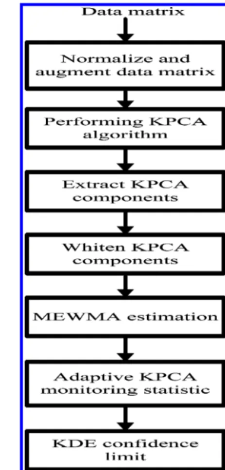
The proposed adaptive KPCA monitoring scheme is sketched in Figure 1. Generally, the proposed method involves three main steps: (1) augmenting the obtained data matrix in order to capture the process dynamic characteristic; (2) whitening the KPCA components to let the covariance matrix to be an identity matrix; (3) Applying MEWMA to capture the time-varying process shifts and then incorporating with KPCA components to develop an adaptive monitoring statistic.
Consider a normalized data matrix (from normal operating condition), the first step is to augment the normalized data matrix with time lag l in order to take into consideration dynamic characteristics, such that
Xl) [X(k) X(k - 1) · · · X(k - l)] )
[
xkT xk+1T l xk+N-1T xk-1T xkT l xk+N-2T · · · · · · l · · · xk-lT xk+1-lT l xk+N-1-lT]
(12)where xkis the normalized observation vector at sample k (k )
1, ..., N). Performing eigenvalue decomposition to the radial basis kernel transformed matrix of Xl, and the centered kernel
matrix (K˜ ) can be further calculated from eq 5. The dimension reduction can be achieved by retaining the largest d eigenvalues (Λ ) diag(λ1, · · · , λd)), associated with eigenvectors (H ) [R1, · · · , Rd]) by using the empirical criterion (Zhang and Qin;24 Zhang25):
λi
sum(λi)> 0.001 (13)
where λiis the ith eigenvalue of K˜ (i ) 1, ..., d). The whitened
KPCA score vector can be obtained by
z ) √NΛ-1HT[k˜(x1, x), · · · , k˜(xN, x)]T (14) Next, the MEWMA is used to predict the time-varying mean shifts:
mk) ωzk+ (1 - ω)mk-1 (15)
where ω is the MEWMA smoothing parameter which satisfies 0 e ω e 1.
To take both the changing magnitude and the direction of time-varying mean shifts into consideration, an adaptive moni-toring statistic is proposed to monitor the nonlinear multivariate process, that is
AT2) |mkTzk| (16) From eqs 14 and 15, it is clear that when ω ) 1 then mk) zk,
and AT2will be simplified to the traditional KPCA monitoring scheme (see eq 8). For ω ) 0, mk) mk-1) · · · ) m0and AT2 will be simplified to a directionally variant T2chart designed for m0(Wang and Tsung26).
Unlike T2, the confidence limit can be determined from
F-distribution. It means that AT2does not follow a specific distribution, and hence a nonparametric technique, kernel density estimation (KDE) is adopted to determine the confidence limit from the normal operating data. Details of the KDE algorithm can be found in Lee et al.27,28 In this
section, we describe the main procedure of the proposed method. The further details of calculation procedures are
described in Appendix A. The procedures are divided into two phases: off-line training and online process monitoring.
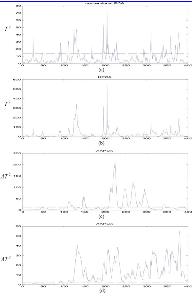
Figure 2. Monitoring results by simulated process. (a) PCA method, (b) KPCA method, (c) adaptive KPCA method with ω ) 0.2, (d) adaptive KPCA
The objective of off-line phase is to build models under normal operating condition, whereas the online phase utilizes the built model to real-time monitor the processes.
4. Implementation
In this section, the proposed method is first implemented in a simulated five-variable nonlinear system. Next, a case study of Tennessee Eastman process is conducted to verify the efficiency of the proposed method. The superiority of the proposed adaptive KPCA method is then demonstrated by comparing with the traditional PCA and KPCA monitoring schemes.
4.1. A Simulated Nonlinear System. In this section, a
five-variable nonlinear system provided by Yoo and Lee21 is implemented to investigate the efficiency of the proposed method. The state space representation of the nonlinear system can be expressed as g(k) )
[
0.118 -0.191 0.287 0.847 0.264 0.943 -0.333 0.514 -0.217]
g(k - 1) +[
1 2 3 -4 -2 1]
u2(k - 1) y(k) ) g(k) + v(k) (17) where y is the output and g is the state. The v is assumed to be normally distributed with zero mean and variance of 0.1. The input u can be expressed asu(k) )
[
0.811 -0.2260.477 0.415
]
u(k - 1) +[
0.193 0.689-0.320 -0.749
]
h(k - 1) (18) where h is a random noise with zero mean and variance of 1.0. All the five variables are involved in the monitoring, including three outputs and two inputs (y1,y2,y3,u1,u2).Under a normal operating condition, 400 simulated samples are used to compare the efficiency of the PCA, KPCA, and adaptive KPCA models. Four components of PCA are selected to explain 80% of the variance. By applying eq 12 to 400 normal operating samples, the components selected for KPCA and adaptive KPCA are 7 and 16, respectively. Same as the work of Yoo and Lee,21the radial basis kernel with parameter σ ) 5m is used for implementing KPCA and adaptive KPCA algorithms. Lee et al.28reported that applying a time-lag value of l ) 1 or 2 to augment the data matrix is usually appropriate to describe the dynamic characteristic of process. Thus, l ) 2 is adopted in the proposed adaptive KPCA method. Besides, Montgomery29 found that the value of ω (i.e., MEWMA smoothing parameter) in the interval 0.05 e ω e 0.25 work well in experience. A good rule of thumb is to use smaller values of ω to detect smaller shifts. Accordingly, ω ) 0.05 and ω ) 0.2 is used in this study.
To compare the detectability of process disturbance of various monitoring methods, a test data set of 400 samples is generated. In which, a step change of h1 (the first element of h) with magnitude of 1.5 is induced in samples 100 to the end (100-400). Figure 2 shows the monitoring results for PCA, KPCA, adaptive KPCA with ω ) 0.2 and adaptive KPCA with
ω ) 0.05. For a fair comparison, the 99% control limits are
used for each method and are sketched with dotted lines. Figure
2 exhibits that KPCA method (detection rate after sample 100 is 41.53%) performs better than PCA (detection rate after sample 100 is 19.27%). However, it is evident that both PCA and KPCA can only fragmentarily detect the step disturbance that occurred after sample 100. Besides, the false alarm rates for PCA and KPCA seem to be high before sample 100, which may be misleading to engineers judging the process status.
Figure 2 panels c and d show that the adaptive KPCA monitoring method can efficiently enhance the ability of the traditional KPCA method for detecting small process disturbance because the proposed AT2 utilizes MEWMA to predict the process mean shifts. Moreover, it shows that AT2with a smaller value of MEWMA parameter can conduct a better result than that with a larger value. The detection rates for AT2with ω ) 0.2 and ω ) 0.05 are 51.16% and 91.02%, respectively. Furthermore, the AT2with ω ) 0.05 (Figure 2c) can successfully distinguish the fault pattern after sample 108 (i.e., a detection delay of 8 samples) and this information helps engineers perform a rectifying action in order to bring the process into a stable situation.
4.2. Tennessee Eastman Process. The Tennessee Eastman
process, created by Eastman Chemical Company, is a complex nonlinear process (Zhang22). Many previous studies imple-mented the TE process for multivariate process monitoring, such as Chen and Liao,30Lee et al.,28,31,32Ge and Song,33Hsu et al.,34and Zhang.22In this section, the efficiency of the proposed method is also verified via monitoring the TE process. Figure 3 sketches the TE process layout. The system contains five major units: a reactor, a condenser, a recycle compressor, a separator, and a stripper. Details can be found in the book of Chiang et al.35The same data set that was generated by Chiang et al.35 will be adopted for analysis. The data set can be downloaded from http://brahms.scs.uiuc.edu.
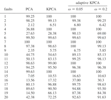
Table 1 lists all the 33 variables which are used for TE process monitoring. A set of programmed faults (Faults 1-21) are listed in Table 2. The normal operating data set (Fault 0) contains 500 samples and is used to build the off-line models. In the test data set, all of the fault types (Fault 1-21) are introduced at sample 160 over 960 observations. The first step for implementing PCA, KPCA, and adaptive KPCA monitoring methods is normalizing the obtained data matrix by the estimated mean and standard deviation from the off-line training phase in Appendix A. The detection rate is used as an index of comparison which measures the percentage of samples outside the 99% control limits after the fault occurrence. For PCA, 16 principal components are selected to explain 80% of the variance. The radial basis kernel is used in the KPCA and adaptive KPCA methods. For adaptive KPCA, l ) 2 is adopted for augmenting the data matrix. By using the criterion of λi/
sum(λi)> 0.001, 25, and 63 principal components are selected
for implementing KPCA and adaptive KPCA methods. Table 3 shows the comparison results of PCA, KPCA, adaptive KPCA with ω ) 0.05 and adaptive KPCA with ω ) 0.2, in terms of detection rates. All methods cannot detect faults 3, 9, 15, and 16 due to the fault magnitude is too small and had almost no effect on the overall process. On the other hand, all methods perform well in detecting faults 1, 2, 6, 7, 8, 12, 13 and 14; the detection rates achieve near 100% performance. Generally, the KPCA (i.e., nonlinear) method performs better than PCA (i.e., linear) method, especially for fault 4, where the reactor cooling water inlet temperature is changed step by step. It is obvious that the adaptive KPCA achieves the best performance for most faults, especially for faults 5, 10, 11, 19, and 20. Further, the adaptive KPCA with smaller MEWMA
parameter (say ω ) 0.05) performs better than that with a larger value (say ω ) 0.2).
Figure 4 shows the monitoring results for faults 5, 10, 11, 19, and 20 by using PCA, KPCA, and adaptive KPCA with ω ) 0.05. It is clear that the proposed adaptive KPCA can efficiently detect the fault types after sample 160. Taking the
Figure 3. Layout of TE process (Downs and Vogel36).
Table 1. Monitored Variables for TE Process
no. process measurements no. process measurements no. manipulated variables
1 A feed (stream 1) 12 product sep level 23 D feed flow (stream 2)
2 D feed (stream 2) 13 prod sep pressure 24 E feed flow (stream 3)
3 E feed (stream 3) 14 prod sep underflow (stream 10) 25 A feed flow (stream 1)
4 A and C feed (stream 4) 15 stripper level 26 total feed flow valve (stream 4)
5 recycle flow (stream 8) 16 stripper pressure 27 compressor recycle valve
6 reactor feed rate (stream 6) 17 stripper underflow (stream 11) 28 purge valve (stream 9)
7 reactor pressure 18 stripper temperature 29 separator pot liquid flow (stream 10)
8 reactor level 19 stripper steam flow 30 stripper liquid product flow (stream 11)
9 reactor temperature 20 compressor work 31 stripper steam valve
10 purge rate (stream 9) 21 reactor cooling water outlet temp 32 reactor cooling water valve 11 product sep temp 22 separator cooling water outlet temp 33 condenser cooling water flow
Table 2. Process Faults for TE Process
fault no. state disturbance
0 no fault no 1 A/C feed ratio, B composition
constant (stream 4)
step 2 B composition, A/C ratio constant
(stream 4)
step 3 D feed temperature (stream 2) step 4 reactor cooling water inlet temperature step 5 condenser cooling water inlet
temperature
step 6 A feed loss (stream 1) step 7 C header pressure loss - reduced
availability (stream 4)
step
8 A, B, C feed composition (stream 4) random variation 9 D feed temperature (stream 2) random variation 10 C feed temperature (stream 4) random variation 11 reactor cooling water inlet temperature random variation 12 condenser cooling water inlet
temperature
random variation 13 reaction kinetics slow drift 14 reactor cooling water valve sticking 15 condenser cooling water valve sticking 16 unknown unknown 17 unknown unknown 18 unknown unknown 19 unknown unknown 20 unknown unknown 21 valve position constant (stream 4) constant position
Table 3. Detection Rates for PCA, KPCA, and Adaptive KPCA
adaptive KPCA
faults PCA KPCA ω ) 0.05 ω ) 0.2
1 99.25 100 100 100 2 98.25 99.13 99.38 99.25 3 2.12 6.51 6.80 6.42 4 36.88 100 100 100 5 27.63 28.38 90.13 69.00 6 99.50 99.63 99.63 99.63 7 100 100 100 100 8 97.38 98.63 100 99.13 9 2.35 5.75 6.75 5.85 10 44.75 54.63 89.13 85.13 11 50.13 83.13 99.25 98.13 12 98.63 99.00 100 100 13 94.25 95.50 96.38 96.38 14 99.63 100 100 100 15 7.05 10.53 16.63 10.63 16 13.56 17.32 37.00 30.3 17 80.13 96.88 99.75 98.63 18 89.63 90.50 94.88 93.50 19 14.50 66.13 87.38 84.38 20 42.38 72.25 92.63 91.63
fault 5 as an example, although PCA and KPCA can im-mediately detect fault 5 at sample 160, the process being back inside the control limit after sample 350 will mislead engineers in judging the process status, whereas the adaptive KPCA method can successfully detect fault 5 after sample 160. Generally speaking, the adaptive KPCA can enhance the detectability of TE process monitoring because the proposed adaptive KPCA method properly takes into consideration of process dynamics and the nonlinear relationship, and it uses MEWMA to predict the process mean shifts.
5. Conclusion
This research developed an adaptive monitoring statistic (AT2) for KPCA to enhance the detectability of small disturbance for
monitoring nonlinear multivariate process. The developed AT2 utilizes MEWMA to estimate the process mean shifts, and then the predicted shift is integrated with the extracted KPCA components. Besides, the AT2based monitoring scheme is also proposed in this study. The proposed scheme takes the process dynamic and nonlinear relationship into consideration. Through implementing two examples, results exhibit that AT2with smaller value of MEWMA parameter can perform better than a larger value. Further, results demonstrate that the proposed monitoring scheme possesses a superior performance when it is compared to the traditional PCA and KPCA methods.
This study shows the superiority of the adaptive KPCA method; however, there are some issues that need to be further addressed. The effectiveness of the proposed method was
Figure 4. (a) Monitoring results of TE process for fault 5, (b) monitoring results of TE process for fault 10, (c) monitoring results of TE process for fault
demonstrated by using the simulated process data. Future work can implement the proposed method with the real-world industrial data, which can additionally include process identi-fication and parameter estimation. For KPCA, the input space is mapped to the feature space and the kernel matrix will become larger when the sample size is increased. Therefore, the development of a preprocessing step in the KPCA method for reducing the computation time is another issue in the future works. Finally, how to select the appropriate kernel function is also an important issue in developing KPCA.
Acknowledgment
This work was supported in part by National Science Council of Taiwan (Grant No. NSC 97-2221-E-324-025).
Appendix
Off-Line Training. The objective of off-line training is to
build a normal operating condition (NOC) model which is developed as follows:
(1) Obtain an NOC data set with m variables and N samples (X∈ RN×m). Normalize the data matrix by the estimated mean
and standard deviation for each variable.
(2) Augment the normalized data matrix by using eq 12, denoted as Xl.
(3) Compute the kernel matrix (K∈ RN×N) to X
lvia the radial
basis kernel function.
(4) Center the kernel matrix (K˜ ) by using eq 5. After that, perform eigenvalue decomposition to K˜ and select the largest
d eigenvalues from eq 12. Thus, the eigenvectors R1, · · · , Rd and the associated eigenvalues λ1g · · · g λdcan be obtained. (5) Whiten the extracted KPCA score vector (z) from eq 13, such that z satisfies E{zzT} ) I.
(6) Given a smoothing parameter ω, apply the MEWMA model to z from eq 14.
(7) Calculate the proposed adaptive monitoring statistic from eq 15.
(8) Determine the KDE based control limit of AT2. Online Monitoring. (1) Obtain a test (or new) data set Xnew ∈ Rm. Normalize X
new with the same estimated mean and standard deviation from NOC modeling step.
(2) Augment the normalized test data set with time lag l. (3) Consider a normalized and augmented test data vector
xt, the kernel vector kt∈ R1×Nat sample t can be calculated by
[kt]j) [kt(xt,xj)], where xjdenotes the jth normal operating data
vector (j ) 1, · · · , N).
(4) Center the kernel vector ktby
k˜t) kt- 1tK - k1N+ 1tK1N (A.1) where K is obtained from step 3 of off-line training procedure and 1t) (1/N)[1, ..., 1] ∈ R1×N.
(5) Calculate the whitened components of test data set by
znew)√NΛ-1HT[k˜t(x1, xt), · · · , k˜t(xN, xt)]T (A.2) (6) Apply the MEWMA to znew, such that
mnew,t) ωznew,t+ (1 - ω)mnew,t-1 (A.3) where ω is the smoothing parameter given from off-line training procedure.
(7) Calculate the adaptive monitoring statistic, that is
ATnew2 ) |mnew,tT znew| (A.4)
(8) Decide whether the ATnew2 exceeds the KDE control limit
in the off-line training procedure.
Literature Cited
(1) Jackson, J. E. Quality control methods for several related variables.
Technometrics 1959, 1 (4), 359–377.
(2) Jackson, J. E.; Mudholkar, G. S. Control procedure for residuals associated with principal component analysis. Technometrics 1979, 21, 341– 349.
(3) Ku, W.; Storer, R. H.; Georgakis, C. Disturbance detection and isolation by dynamic principal component analysis. Chemom. Intell. Lab.
Syst. 1995, 30, 179–196.
(4) Tsung, F. Statistical monitoring and diagnosis of automatic controlled processes using dynamic PCA. Int. J. Prod. Res. 2000, 38 (3), 625–637.
(5) Hubert, M.; Rousseeuw, P. J.; Vanden Branden, K. ROBPCA: A new approach to robust principal component analysis. Technometrics 2005,
47 (1), 64–79.
(6) Hubert, M.; Rousseeuw, P.; Verdonck, T. Robust PCA for skewed data and its outlier map. Comput. Stat. Data Anal. 2008, 53 (6), 2264– 2274.
(7) Nomikos, P.; MacGregor, J. F. Monitoring batch processes using multiway principal component analysis. Am. Inst. Chem. Eng. J. 1994, 40, 1361–1375.
(8) Nomikos, P.; MacGregor, J. F. Multivariate SPC charts for monitor-ing batch processes. Technometrics 1995, 37, 41–59.
(9) Bakshi, B. R. Multiscale PCA with application to multivariate statistical process monitoring. AIChE J. 1998, 44 (7), 1596–1610.
(10) Li, W.; Yue, H.; Cervantes, S. V.; Qin, T. Recursive PCA for adaptive process monitoring. J. Process Control 2000, 10, 471–486.
(11) Shi, D.; Tsung, F. Modelling and diagnosis of feedback-controlled processes using dynamic PCA and neural networks. Int. J. Prod. Res. 2003,
41 (2), 365–379.
(12) Cho, H. W.; Kim, K. J.; Jeong, M. K. Multivariate statistical diagnosis using triangular representation of fault patterns in principal component space. Int. J. Prod. Res. 2005, 43 (24), 5181–5198.
(13) Kramer, M. A. Non-linear principal component analysis using autoassociative neural networks. AIChE J. 1991, 37, 233–243.
(14) Dong, D.; McAvoy, T. J. Nonlinear principal component analysis based on principal curves and neural networks. Comput. Chem. Eng. 1996,
20, 65–78.
(15) Hastie, T. J. Stuetzle. Principal curves. J. Am. Stat. Assoc. 1989,
84, 502–516.
(16) Tan, S.; Mavrovouniotis, M. L. Reducing data dimensionality through optimizing neural networks inputs. AIChE J. 1995, 41, 1471– 1480.
(17) Jia, F.; Martin, E. B.; Morris, A. J. Non-linear principal component analysis for process fault detection. Comput. Chem. Eng. 1998, 22, S851– S854.
(18) Scho¨lkopf, B.; Smola, A. J.; Mu¨ller, K. J. Nonlinear component analysis as a kernel eigenvalue problem. Neural Comput. 1998, 10 (5), 1299– 1399.
(19) Lee, J. M.; Yoo, C. K.; Choi, S. W.; Vanrolleghem, P. A.; Lee, I. B. Nonlinear process monitoring using kernel principal component analysis. Chem. Eng. Sci. 2004d, 59, 223–234.
(20) Choi, S. W.; Lee, C. K.; Lee, J. M.; Park, J. H.; Lee, I. B. Fault detection and identification of nonlinear processes based on kernel PCA.
Chemom. Intell. Lab. Syst. 2005, 75, 55–67.
(21) Yoo, C. K.; Lee, I. B. Nonlinear multivariate filtering and bioprocess monitoring for supervising nonlinear biological process. Process Biochem.
2006, 41, 1854–1863.
(22) Zhang, Y. Enhanced statistical analysis of nonlinear processes using KPCA, KICA, and SVM. Chem. Eng. Sci. 2009, 64, 801–811.
(23) Mika, S.; Scho¨lkopf, B.; Smola, A. J.; Mu¨ller, K. J.; Scholz, M.; Ra¨tsh, G. Kernel PCA and de-nosing in feature spaces. Proc. AdV. Neural
Inform. Process. Syst. II 1999, 536–542.
(24) Zhang, Y.; Qin, S. J. Fault detection of nonlinear processes using multiway kernel independent component analysis. Ind. Chem. Res. 2007,
46, 7780–7787.
(25) Zhang, Y. Fault detection and diagnosis of nonlinear processes using improved kernel independent component analysis (KICA) and support vector machine (SVM). Ind. Chem. Res. 2008, 47, 6961–6971.
(26) Wang, K.; Tsung, F. An adaptive T2chart for monitoring dynamic
systems. J. Qual. Technol. 2008, 40 (1), 109–123.
(27) Lee, J. M.; Yoo, C. K.; Lee, I. B. Statistical process monitoring with independent component analysis. J. Process Control 2004a, 14, 467– 485.
(28) Lee, J. M; Yoo, C. K.; Lee, I. B. Statistical monitoring of dynamic processes based on dynamic independent component analysis. Chem. Eng.
Sci. 2004b, 59, 2995–3006.
(29) Montgomery, D. C. Introduction to Statistical Quality Control, 3rd ed.; John Wiley & Sons, Inc.: New York, 1996.
(30) Chen, J.; Liao, C. M. Dynamic process fault monitoring based on neural network and PCA. J. Process Control 2002, 12, 277–289.
(31) Lee, J. M; Qin, S. J.; Lee, I. B. Fault detection and diagnosis based on modified independent component analysis. AIChE J. 2006, 52 (10), 3501– 3514.
(32) Lee, J. M.; Qin, S. J.; Lee, I. B. Fault detection of non-linear processes using kernel independent component analysis. Can. J. Chem. Eng.
2007, 85, 526–536.
(33) Ge, Z.; Song, Z. Process monitoring based on independent component analysissprincipal component analysis (ICA-PCA) and simi-larity factors. Ind. Eng. Chem. Res. 2007, 46, 2054–2063.
(34) Hsu, C. C.; Chen, L. S.; Liu, C. H. A. Process monitoring scheme based on independent component analysis and adjusted outliers. Int. J. Prod.
Res. 48 (6), 1727–1743.
(35) Chiang, L. H.; Russell, E. L.; Braatz, R. D. Fault detection and
Diagnosis in Industrial Systems; Springer: London, 2001.
(36) Downs, J. J.; Vogel, E. F. A plant-wide industrial process control problem. Comput. Chem. Eng. 1993, 17 (3), 245–255.
ReceiVed for reView April 1, 2009 ReVised manuscript receiVed November 18, 2009 Accepted November 24, 2009