A Design of a Vortex Flow Data Management
and Analysis System
*TYNE LIANG AND YAN-DUNG HUNG Department of Computer and Information Science
National Chiao Tung University Hsinchu, 300 Taiwan
In this paper, a flow data management and analysis system that can automatically extract features and present summaries of flow fields for the researcher was presented by applying information extraction and mining techniques. The informative vortex features were extracted by using a content-based feature extractor. Shot detection was imple-mented on the basis of a Maximum-Block-Difference method and global clustering was implemented with semi-Hausdorff distance measure. On the other hand, the frequent patterns in data sequences and the hidden relations among visual features were also dis-covered by the application of mining techniques. The implementation of this system is believed to benefit both the information scientist in the context of knowledge discovery and at the same time help develop a good data management system for fluid dynamists to better deal with flow data.
Keywords: data mining, clustering, feature extraction, database, vortex flow
1. INTRODUCTION
Due to the advance in technology, the capabilities of collecting, generating and stor-ing data grow much faster than our abilities to analyze, summarize and extract useful knowledge from them. Although database technology has provided us with the basic tools for efficient storage and lookup for large data sets, it still remains a challenge to analyze and manage large bodies of data effectively.
Contrast to high diversity of the information and knowledge of corpus in natural languages, most scientific database are collected with some specific purpose so that the information and the possible knowledge are comparatively restricted and predictable in some aspects. Moreover, the data structure in a scientific database is relatively simpler and it is usually highly correlated. For example, the flow data obtained by researchers of computational fluid dynamics (CFD) are time varying velocity field composed of three real numbers in each point in space and hence, their temporal and spatial variations are clearly correlated. Therefore, it is possible to design a data management system of large scientific database for efficient information retrieval.
In computational fluid dynamics, the Navier-Stokes equation [14] is solved numeri-cally under different physical situations. The outcomes of the computation are the veloc-ity and pressure fields. For 100 × 100 lattice points in R2, there will be 30,000 double
precision real numbers (20,000 for the velocity field and 10,000 for the pressure field) Received March 14, 2005; revised June 15, 2005; accepted August 24, 2005.
Communicated by Ming-Syan Chen.
* This paper was partially supported by the National Science Council of Taiwan, R.O.C., under grant No.
generated at each time step. If a double precision number occupies 16 bytes, the size of a flow field data file will be 500 Kilobytes. Typically, in one single run, calculation of more than 106 time steps are needed and 1012 bytes of data will be generated. For three-
dimensional problems, the amount of data will be of order 1018 bytes! Thus, it is
impos-sible to record and analyze every calculated flow field for each time step. Usually, only flow field values at some chosen spatial points and flow fields at some chosen time are recorded. The rest of the flow data, which are obtained by more than 99.99% of the com-putation, are discarded without analysis. One of the reasons for such waste was because massive data storage device was not available in the past. Today, with the advance in storage technology, disk arrays of 1012 bytes become affordable and it is possible to store
every bit of the flow field data. However, it remains a difficult task to manage and ana-lyze such huge amount of data. Imagine one flow field is transformed into one video frame and one can examine 30 images in one second (video frame rate). Then more than an hour is needed to examine one typical run. Obviously not every bit of the flow field data contains relevant information wanted by the researcher. It becomes a tedious and time consuming job for an expert to go through the flow field data, identify useful fea-tures and pick out the relevant flow fields for further analysis.
Although there are commercially available software packages (such as TECPLOT and FIELDVIEW) to help the researchers to examine the flow field data, their functions are data visualization and animation, data plotting and data file format conversion. Even with the help of these expensive packages, an expert may miss some useful and critical features of the flow field data due to human error and fatigue. Hence, this paper presents a flow data management and analysis system that can automatically identify features and extract relevant flow fields by employing the techniques of feature extraction, shot detec-tion, global clustering and data mining. The results have been verified by the help of Pro-fessor M. J. Chern (National Taiwan University of Science and Technology) who pro-vided us the flow field data.
The remainder of this paper is organized as follows. Section 2 introduces the vortex flow data. Section 3 describes in details the proposed system architecture and the imple-mentation of the four major function modules. Final conclusion is made in section 4.
2. VORTEX FLOW DATA
Fluid flows are governed by three fundamental laws in fluid mechanics: the mass conservation law, the Newton’s second law of motion known as Navier-Stokes equations, and the energy conservation law. These three laws constitute a set of physical constraints that are different from those commonly used in the study of solid motion. A 2D fluid is completely characterized by a set of parameters {u(x, t), p(x, t)}, where u = {ui, i = 1, 2} is the velocity vector, x = {xi, i = 1, 2} is the spatial coordinate, t is the time, and p is the pressure. The fluid data can be obtained by either CFD simulation or experiments, such as Particle Imaging Velocimetry (PIV). Moreover, the fluid data obtained from PIV ex-periments contain only velocity fields at different time instants. In this paper, the data given are velocity fields of 2D cavity flows obtained from CFD.
The velocity fields are vectors defined on a set of discrete points, {u(xk)}, where xk ∈ D ⊂ R2. In practice, D can be a set of regular lattice points, or a set of random points.
In this paper, D is a set of regular lattice points and each dimension contains 51 points. Fig. 1 (a) shows a velocity field obtained from CFD, and it is called velocity image. For the convenience to observe the properties of vortices in fluid at each time instant, such as vortex position, size and … etc., stream function [14] is used and it is defined as:
( , )
x y
S x y =
∫
vdx+∫
udy (1) where u is the velocity in x, and v is the velocity in y. The lines along which the stream function is a constant are called streamlines. These are lines whose tangents are every-where parallel to the velocity vector. Fig. 1 (b) is the corresponding streamline image. So displaying image of every time instant according to time line, we can get the corre-sponding velocity video and streamline video.Fig. 1. (a) The 2D velocity field in cavity. The
original field is of 51 × 51 resolution. Fig. 1. (b) The corresponding stream function contour.
3. THE PROPOSED SYSTEM
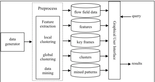
The presented system, as shown in Fig. 2, is composed of data generator, the graphi-cal user interface and four other task modules. The data generator is a CFD flow data simulation program which generates the flow field data. The graphical user interface eases user’s processing, browsing and searching data. Other four function modules are for feature extraction, local clustering, global clustering and data mining. The feature extraction is implemented to extract both visual and statistical features of flow field data at each time instant and the extracted features are stored in feature database. The local clustering is functioned as shot detection so that we can segment flow field data into temporal segments and a frame from each segment will be selected as a key frame. Global clustering is to group data into clusters for overall summarization and the data mining module is to discover from clustering results some interesting patterns and extract implicit association rules.
The proposed system was encoded in Interactive Data Language (IDL), a platform independent language, making it possible to transport our system to different kinds of operation system platforms with few modifications. The main system window, support-ing six command buttons, namely Input File, Preprocess, Frame Display, Search, Clus-tering, Data Miner, and Exit, and a message bar at the bottom. Clicking each of the commands will activate the corresponding procedures. For example, Fig. 3 is the result
Preprocess
data generator
flow field data
features key frames clusters mined patterns G ra phic al U se r Inte rfa ce query results Feature extraction local clustering global clustering data mining
Fig. 2. The system architecture.
Fig. 3. A local clustering results.
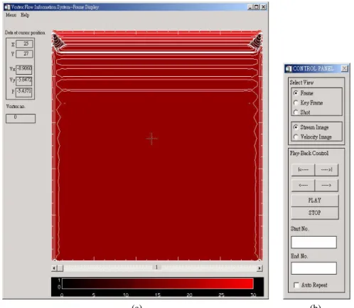
window of performing local clustering. The curves shown in this window indicate the variation of number of visual features from each key frame and the message in the win-dow tells how many key frames (each shot will be represented with one key frame) are generated after local clustering. While users clicking “frame display” in the main win-dow, the display window and control panel window will be shown as Fig. 4 where users can move the cursor to any place on the drawing area. The control panel window is used to control the display modes of frame display window. User can select to view the streamline image or velocity image of a specific frame by clicking the image type button in control panel window. Fig. 5 is one result of processing global clustering and it shows
(a) (b) Fig. 4. The frame-display window and control-panel window.
the statistical information for each cluster. As shown in this figure, clicking the frame number in the frame list of a selected cluster will have the streamline image of the se-lected frame shown on the draw area.
3.1 Feature Extraction
Feature extractor extracts both visual features and statistical features from each frame. These features are then encoded in feature vectors, which in turn are used as indi-ces for frame search. Four basic visual features are concerned and extracted from a frame, namely vortex center, vortex size, separation point, and stagnation point.
Three properties can be used to extract vortex center and size. First, a vortex center occurs at sampling points with local maximum or minimum stream values. Second, the stream values of these points belonging to the same vortex will decrease or increase from vortex center to vortex boundary. Third, the stream values of the points at vortex bound-ary approximate to zero. Based on these properties, we use the Peak Climbing Method [8] to extract vortex centers and sizes from each image frame as follows:
(1) Compute the absolute stream value of each pixel of the current frame.
(2) For each pixel P, search P and its eight neighboring points and find the point Q hav-ing maximum stream value. If P ≠ Q, make a link from P to Q.
(3) Find those pixels, which have no link to other points, and label them as vortex cen-ters.
(4) Count number of pixels linked together to each founded vortex center as the vortex size of that vortex.
Flow separation points occur in the place where one streamline separates into two streamlines. So separation points occur when the stream value of one point is the same as that of more than one of its eight neighboring points. This property makes one flow sepa-rate into two flows. Besides, separation points occur at vortex boundaries. So vortex boundaries can be identified by checking whether two neighboring points belonging to different vortices; then separation points are extracted by scanning vortex boundaries and verifying whether any vortex separation point occurs or not.
Flow stagnation points occur in the place where their velocity values become zero. Due to frame resolution, stagnation points may appear at the same position of one sam-pling point, or appear between two adjacent samsam-pling points, or appear in four neighbor-ing points. So stagnation points will be identified by scannneighbor-ing all the samplneighbor-ing points within a flow field and by checking the cases mentioned previously. Beside the visual features mentioned above, statistical features for each frame are also concerned at frame comparison. In the presented system, each frame is divided into 3 × 3 equal size blocks from which its six statistical values are recorded in a 54-dimesion statistical feature vec-tor. These features include the mean and variance of velocity in x, the mean and variance of velocity in y, and the mean and variance of a stream value.
3.2 Local Clustering
data into temporal segments and a middle frame of a shot is selected as a key frame, pre-senting a local summary. In past literature, many of shot detection methods [10, 17, 18] in uncompressed video domain were presented on the basis of comparing the similarity between adjacent frames and the similarities were calculated by using different kinds of features. Other sophisticated approaches based on shot activity or using application of unsupervised clustering were addressed in [3] and [19] respectively. In this paper, a con-tent-based shot detection method, Maximum-Block-Difference method (MBD), was pre-sented as shown in Fig. 6 where each frame is divided into 3 × 3 equal size blocks, marked from upper left to lower right and line by line, as B1, B2, …, B9. This is because
there may be local variation or repeated patterns in adjacent frames of the test data. Us-ing the difference function (Eq. (2)), we can measure the difference between two frames as follows:
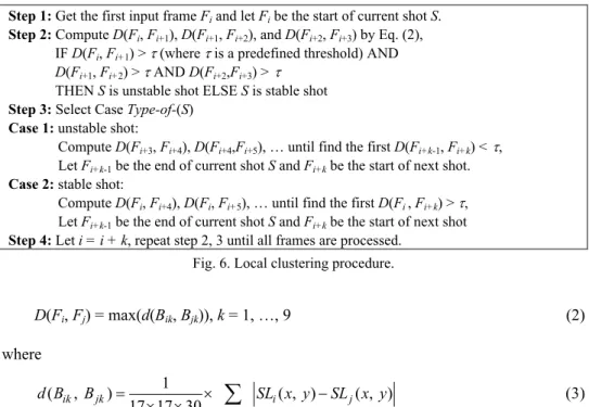
Step 1: Get the first input frame Fi and let Fi be the start of current shot S.
Step 2: Compute D(Fi, Fi+1), D(Fi+1, Fi+2), and D(Fi+2, Fi+3) by Eq. (2), IF D(Fi, Fi+1) > τ (where τ is a predefined threshold) AND
D(Fi+1, Fi+2) > τ AND D(Fi+2,Fi+3) > τ THEN S is unstable shot ELSE S is stable shot
Step 3: Select Case Type-of-(S) Case 1: unstable shot:
Compute D(Fi+3, Fi+4), D(Fi+4,Fi+5), … until find the first D(Fi+k-1, Fi+k) < τ, Let Fi+k-1 be the end of current shot S and Fi+k be the start of next shot.
Case 2: stable shot:
Compute D(Fi, Fi+4), D(Fi, Fi+5), … until find the first D(Fi , Fi+k) > τ, Let Fi+k-1 be the end of current shot S and Fi+k be the start of next shot
Step 4: Let i = i + k, repeat step 2, 3 until all frames are processed.
Fig. 6. Local clustering procedure.
D(Fi, Fj) = max(d(Bik, Bjk)), k = 1, …, 9 (2) where , 1 ( , ) ( , ) ( , ) 17 17 30 k ik jk i j x y B d B B SL x y SL x y ∈ = × − × ×
∑
(3)where Bik is the kth block of frame i, and SLi(x, y) is the stream level at (x, y) of frame i. The stream level of each pixel is converted from its stream level on the basis of value distribution. Based on the difference measurement, a shot is defined as unstable shot if all its pairs of adjacent frames contain changing block(s) in which d(Bi,k, Bj,k) is greater than a threshold (Eq. (3)) for any pair of adjacent frames Fi and Fj. Otherwise, the shot is treated as a stable shot. The details of MBD, involving type identification of current shot and the shot boundary identification, are described as following Fig. 6.
The performance of the proposed detector was examined with a set of two thousand frames and compared to two other approaches, namely Adjacent-Pair-Comparison method (APC) and First-Frame-Based-Comparison method (FFC). A shot boundary is declared
for APC when its difference between two adjacent frames exceeds a threshold value. On the other hand, FFC will calculate the difference between the first frame and the follow-ing frames. The calculation will be made till Fk whose D(Fi, Fk) is greater than a thresh-old. A shot boundary is declared at Fk-1, and Fk will be the first frame of the next shot.
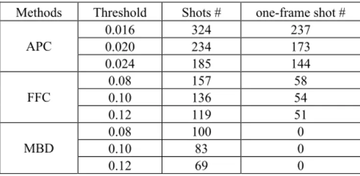
Table 1 lists experimental results for APC, FFC, and MBD methods and they were verified by domain experts. It is found that APC yields many consecutive one-frame shots throughout the whole dataset while FFC produces many one-frame shots only when the test data have more fluctuations. However, FFC does not handle the case well when the data contain repeated patterns of frames. On the other hand, the results from MBD method show that it is capable to deal with repeated patterns. So MBD method was embedded into our system as local clusters generator. From our experiments, the thresh-old value of MBD within the range from 0.08 to 0.16 yielded better results which contain less number of one-shot frame and their shot boundaries are close to the manual judg-ment.
Table 1. Shot detection results comparisons.
Methods Threshold Shots # one-frame shot #
0.016 324 237 0.020 234 173 APC 0.024 185 144 0.08 157 58 0.10 136 54 FFC 0.12 119 51 0.08 100 0 0.10 83 0 MBD 0.12 69 0
5. THE GLOBAL CLUSTERING
The global clustering methods are used to capture the salient content of a set of flow field data as well as to mine from them the patterns and association rules. Among differ-ent clustering algorithms presdiffer-ented in past years, K-means algorithm [13] is famous for its easy implementation, yet it may stick in local optimal solution. To solve it, sequential search approach like simulated annealing (SA) [12], parallel approaches like genetic al-gorithm (GA) [6], and evolutionary programming (EP) [5] were proposed. Though par-allel methods speedup their search for optimal solution, they are hard to implement and require large storage space. In addition, their quality of clustering results is highly fected with the design of fitness function and mutation function, which in turn are af-fected by the type of data sets.
In this paper, a clustering algorithm applicable for our data sets is presented on the basis of semi-Hausdorff distance measure [4]. There are two benefits associated with this algorithm. First, it does not need a priori, the number of clusters, presented in the given data set. Moreover, it finds out the optimal number of clusters in the given data set. Sec-ond, there is a relation between the predefined distance threshold and quality of the re-sults produced, making it tunable for different performance requirements.
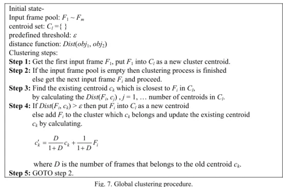
The distance function Eq. (2) is used to measure the distance between two frames. Although the clustering result of this algorithm is sub-optimal solution, its merits are fast computation and easy implementation. Fig. 7 describes its implementation steps in de-tails.
Initial state-
Input frame pool: F1 ~ Fm centroid set: Cl ={ } predefined threshold: ε
distance function:Dist(obj1, obj2)
Clustering steps:
Step 1: Get the first input frame F1, put F1 into Cl as a new cluster centroid.
Step 2: If the input frame pool is empty then clustering process is finished
else get the next input frame Fi and proceed.
Step 3: Find the existing centroid ck which is closest to Fi in Cl,
by calculating the Dist(Fi, cj) , j = 1, … number of centroids in Cl.
Step 4: If Dist(Fi, ck) > ε then put Fi into Cl as a new centroid
else add Fi to the cluster which ck belongs and update the existing centroid ck by calculating. 1 1 1 k k i D c c F D D ′ = + + +
where D is the number of frames that belongs to the old centroid ck.
Step 5: GOTO step 2.
Fig. 7. Global clustering procedure.
Table 2. The global clustering results.
ε = 0.05 ε = 0.10 ε = 0.15
Data Set Number of clusters Time (Seconds) Number of clusters Time (Seconds) Number of clusters Time (Seconds) 1 148 380 57 168 30 100 2 23 86 10 47 6 37 3 18 71 10 46 6 36 4 28 89 16 57 9 45
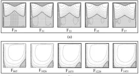
In the experiments, four data sets, each containing two thousand frames, were used to validate the effectiveness of the proposed approach. The first data set contains more diversities than the others, so it has more clusters after global clustering. Table 2 shows the clustering statistics for different thresholds. Fig. 8 shows two examples of clusters obtained from data set one using ε = 0.10. It is reasonable that the frames in Fig. 8 (a) are in the same cluster because they are consecutive frames. Such clusters can be easily picked out manually when browsing through the images. On the other hand, the frames in Fig. 8 (b) are scattered within the data set, they will be difficult to be picked manually without the use of the clustering algorithm.
F29 F31 F33 F35 F37
(a)
F865 F1026 F1075 F1229 F1431
(b)
Fig. 8. Examples of two global clusters from dataset 1.
6. THE DATA MINER
As clusters useful for summarizing vortex flow data which are highly correlated with spatial and temporal variations, their frequent patterns and implicit association rules among various kinds of features in frames are also interesting to the researchers of fluid dynamics. Hence, the proposed system is embedded with a data miner which is based on the well-known Apriori algorithm, an efficient association rule mining method in the field of sequential pattern mining [1, 2].
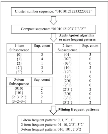
The frequent patterns were mined in such a way that each frame is first encoded with the cluster number generated during global clustering procedure. Then a sequence, for example “010101212233223322”, is generalized to be a compact list “010101212+3+
2+3+2+” where + refers to the repeats. Finally, those frequent patterns from the example
sequence, (as shown in Fig. 9 where the minimum support number is 2) can be mined from the compact list by using Apriori algorithm. The algorithm employs breadth-first search and uses a hash tree structure to count candidate patterns efficiently. The candidate patterns of length k are generated from k − 1 length patterns, and then, the patterns which have an infrequent sub-pattern are pruned.
On the other hand, the presented miner will mine the strong association rules (which satisfy both a minimum support threshold and a minimum confidence threshold) among visual features and statistical features. Because the data type of association rule mining requires nominal data, statistical features are transformed using following equations.
min 10 max min f f f v v′ =INT⎛⎜⎜ − × ⎞⎟⎟ − ⎝ ⎠ (4) where minf and maxf are the minimum value and maximum value of feature f and INT() is a function to translate floating point decimals to integer value. This equation maps a value v of the feature f to an integer v′ in the range [0, 10].
3-item Subsequence Sup. count {010} 2 {101} 2 {2+3+2+} 2 {3+2+3+} 1
Cluster number sequence: “010101212233223322”
Compact sequence: “010101212+3+2+3+2+” 2-item Subsequence Sup. count {01} 3 {02+} 0 {03+} 0 {10} 2 {12+} 1 {13+} 0 {2+0} 0 {2+1} 0 {2+3+} 2 {3+0} 0 {3+1} 0 {3+2+} 2
1-item frequent pattern: 0, 1, 2+, 3+ 2-item frequent pattern: 01, 10, 2+3+, 3+2+ 3-item frequent pattern: 010, 101, 2+3+2+
Apply Apriori algorithm to mine frequent patterns
Mining frequent patterns
1-item Subsequence Sup. count {0} 3 {1} 4 {2} 1 {2+} 3 {3+} 2
Fig. 9. An example flow chart of mining frequent patterns.
Table 3. Five mined association rules from data set 1.
Association Rule Support Confidence C[1] => S[0] 8.95 99.44 C[2] => S[2] 19.25 99.48 C[3] => S[4] 20.50 92.14 C[4] => S[6] 16.90 81.45 C[5] => S[8] 14.45 87.90
The experiments were implemented with data set one which contains two thousands of frames. The results show that some frequent pattern like “5354” (key frame of cluster number 53 and key frame of cluster 54) was found in three different places: between the 995th frame and the 1097th frame, between 1206th frame and 1297th frame, and between 1385th frame and 1457th frame. Such pattern was also observed when we scanned through the test frame manually. On the other hand, some association rules shown in Table 3 were extracted with a minimum support threshold value 5% and a minimum confidence value 85%. The notation C[1] refers to number of vortex centers is 1, and S[0] refers to number of separation points is 0. From these rules, we could understand the relationship among number of vortices and number of separation points. As shown in Table 3, the
total support of these five rules is greater than 80% of the samples, so we could conclude that there is a strong connection between the vortex centers and separation points.
From the experimental results described above, our approach could appropriately mine frequent patterns and strong association rules from a set of vortex flow data cor-rectly. However, the results are based on the global clustering results, therefore different frequent patterns may be obtained by implementing different global clustering threshold parameter.
7. CONCLUSIONS
With rapid growth of computer technology, various communities have accumulated increasingly large amount of data. Hence there is an urgent need to automatically manage, analyze, summarize and extract useful knowledge from them. In this paper, we imple-ment a prototype system to automatically manage and analyze vortex flow data by ap-plying information extraction and mining techniques. The system is able to support the following functions:
(a) Efficient management of vortex flow data. The feature extractor correctly extracts the visual features and statistical features of flow field data at each time instant, and these extracted features are indexed for the search needs.
(b) Data summarization. The global and local clusters can provide information such as summary of each shot, preview of whole data set, and main data types of whole data set.
(c) Friendly user interface. The proposed system provides a graphical user interface for users to interact with the system.
(d) Basic knowledge acquisition. The data miner of the proposed system is able to mine the frequent patterns and association rules from flow field data.
Future works include the exploration of novel techniques useful to mine frequent patterns with multiple time constraints.
ACKNOWLEDGEMENT
We would like to thank Dr. Kiwing To, Institute of Physics of Academia Sinica, Taipei, Taiwan for giving us precious suggestions on constructing the presented proto-type system. Thanks also go to Professor M. J. Chern, Department of Mechanical Engi-neering, National Taiwan University of Science and Technology, for providing us the test data sets and helping our verification of the experimental results.
REFERENCES
1. R. Agrawal, T. Imielinski, and A. Swami, “Mining association rules between sets of items in large databases,” in Proceedings of ACM SIGMOD International
2. R. Agrawal and R. Srikant, “Fast algorithms for mining association rules in large databases,” in Proceedings of the International Conference on Very Large Data
Bases, 1994, pp. 487-499.
3. Y. S. Avrithis, A. D. Doulamis, N. D. Doulamis, and S. D. Kollias, “A stochastic framework for optimal key frame extraction from MPEG video databases,”
Com-puter Vision and Image Understanding, Vol. 75, 1999, pp. 3-24.
4. H. S. Chang, S. Sull, and S. U. Lee, “Efficient video indexing scheme for content- based retrieval,” IEEE Transactions on Circuits and Systems for Video Technology, Vol. 9, 1999, pp. 1269-1279.
5. D. B. Fogel, “An introduction to simulated evolutionary optimization,” IEEE
Trans-actions on Neural Networks, Vol. 5, 1994, pp. 3-14.
6. D. E. Goldberg, Genetic Algorithms in Search, Optimization and Machine Learning, Addison-Wesley, Reading, MA, U.S.A., 1989.
7. J. Han and M. Kamber, Data Mining: Concepts and Techniques, Morgan Kaufmann, San Francisco, CA, U.S.A., 2001.
8. A. K. Jain and R. C. Dubes, Algorithm for Clustering Data, Prentice-Hall, New Jer-sey, 1988.
9. L. Kaufman and P. J. Rousseeuw, Finding Groups in Data: An Introduction to
Clus-ter Analysis, John Wiley & Sons, New York, U.S.A., 1990.
10. A. Nagasaka and Y. Tanzka, “Automatic video indexing and full-video search for object appearances,” Transactions of Information Processing Society of Japan, Vol. 33, 1992, pp. 543-550.
11. J. R. Quinlan, C4.5: Programs for Machine Learning, Morgan Kaufmann, San Mateo, CA, U.S.A., 1993.
12. S. Z. Selim and K. A. Sultan, “A simulated annealing algorithm for the clustering problem,” Pattern Recognition, Vol. 24, 1991, pp. 1003-1008.
13. J. Tou and R. Gonzalez, Pattern Recognition Principles, Addison-Wesley, Reading, MA, U.S.A., 1974.
14. D. J. Tritton, Physical Fluid Dynamics, Oxford University Press, New York, 1988. 15. J. T. L. Wang, G. Chirn, T. G. Marr, B. A. Shapiro, and K. Zhang, “Combinatorial
pattern discovery for scientific data: some preliminary results,” in ACM Proceedings
of SIGMOD Conference, 1994, pp. 115-125.
16. S. M. Weiss and C. A. Kulikowski, Computer Systems That Learn: Classification
and Prediction Methods from Statistics, Neural Nets, Machine Learning and Expert Systems, Morgan Kaufmann, San Mateo, CA, U.S.A., 1991.
17. R. Zabith, J. Miller, and K. Mai, “Feature based algorithms for detecting and classi-fying scene breaks,” in Proceedings of the 4th ACM International Conference on
Multimedia, 1995, pp. 189-200.
18. H. J. Zhang, “Automatic partitioning of full-motion video,” Multimedia Systems, Vol. 1, 1993, pp. 82-100.
19. Y. Zhuang, Y. Rui, T. S. Huang, and S. Mehrotra, “Adaptive key frame extraction using unsupervised clustering,” in Proceedings of International Conference on
Tyne Liang (梁婷) received her Ph.D. in Computer Science from National Chiao Tung University, Taiwan, in 1995. Cur-rently she is associate professor of Department of Computer Sci-ence, National Chiao Tung University. Her research interests are information retrieval and processing, natural language processing and interconnection network.
Yang-Dung Hung (洪炎東) was born in Taipei, Taiwan and
obtained his master degree in Computer Science at National Chiao Tung University in 2002. Currently he is working as senior engineer in Technical Develop Department of Sitronix Technol- ogy Corp., Taiwan.