具缺漏值的自發性通報系統資料公開之隱私保護技術

國立高雄大學資訊工程學系

碩士論文

具缺漏值的自發性通報系統資料公開之隱私保護技術

Privacy-Preserving SRS Data Publishing with Missing

Values

研究生：許絖詠 撰

指導教授：林文揚 博士

致謝

具缺漏值的自發性通報系統資料公開之隱私保護技術

MS(k, θ*)-bounding 模型以及 Closed k-anonymity 與 Closed l-diversity 模型，提出 新 的 隱 私 保 護 模 型 Closed MS(k, θ*)-bounding 及 三 種 新 的 隱 私 方 法 ： Closed-MSpartition、Closed-MSdirect、Closed-MSsorting，以處理具有缺漏值的SRS 資

料。

及資料的可用性進行實驗與比較。結果顯示 Closed-MSdirect在資訊失真程度、隱

私 暴 露 風 險 與 資 料 的 可 用 性 都 具 有 較 好 的 表 現 。 雖 然 Closed-MSpartition 與

Closed-MSsorting 的資訊失真程度及隱私暴露風險比 Closed-MSdirect 來的較為高，

而資料的可用性較低，但是仍然在能夠接受的範圍。整體而言，針對 SRS 資料 的缺漏值佔據極大比例的現象，我們提出的新方法可以有效的進行處理以防止攻 擊者竊取個人隱私。

Privacy-Preserving SRS Data Publishing

with Missing Values

Advisor: Dr. (Professor) Wen-Yang Lin

Department of Computer Science and Information Engineering National University of Kaohsiung

Student: Kuang-Yung Hsu

Department of Computer Science and Information Engineering National University of Kaohsiung

Abstract

In recent years, many countries have established Spontaneous Reporting System (SRS) for the detection and analysis of adverse drug reactions (ADRs), such as the US Food and Drug Administration's Adverse Event Reporting System (FAERS). These SRS data usually contain sensitive personal privacy information. In order to prevent personal privacy leakage, the data must be de-identified and processed by some Privacy Protection Data Publishing (PPDP) before being published.

Although many scholars have proposed various privacy protection models, they overlooked characteristics of SRS data. Therefore, our lab proposed a feasible privacy model MS(k, θ*)-bounding dedicate to SRS data and corresponding anonymization method MS-Anonymization. However, this method is only applicable to complete data, not considering the fact that there is lot amount of missing data.

On the other hand, our lab proposed privacy models for handling missing values, Closed k-anonymity and Closed l-diversity, but not dedicate to the characteristics of SRS data. Therefore, in this thesis, we propose a new privacy model Closed MS(k,

Closed l-diversity, and propose three new anonymization methods, Closed-MSpartition,

Closed-MSdirect, Closed-MSsorting,to process SRS data with missing values.

We used FAERS data to test and compare our three methods from the aspects of information loss, privacy risk, and data utility. The results show that Closed-MSdirect

has better performance on information distortion, privacy exposure risk and data utility. Although Closed-MSpartition and Closed-MSsorting have higher information loss

and privacy risk, and lower data utility than Closed-MSdirect, the results are still in

acceptable range. In summary, in the case of a large proportion of SRS contain missing values, our proposed new methods can effectively prevent attackers from learning personal privacy.

Keywords: adverse drug reaction, data anonymization, privacy preserving data

Content

致謝 ... i

摘要 ... ii

Abstract ... iv

List of Tables ... viii

List of Figures ... ix

Chapter 1 Introduction ... 1

1.1 Motivation ... 1

1.2 Contributions ... 2

1.3 Thesis Organization ... 2

Chapter 2 Background Knowledge ... 4

2.1 Privacy Attacks and Privacy Models ... 4

2.2 Anonymization Methods ... 8

Chapter 3 Problem Statement ... 9

3.1 Characteristics of SRS Data ... 9

3.1.1 Missing Values ... 9

3.1.2 Other Features ... 10

3.2 Problems of Current Anonymization Approaches ... 11

Chapter 4 The Proposed Privacy Model and Algorithm ... 14

4.1 Closed MS(𝒌, 𝜽 ∗)-bounding ... 14

4.2 Anonymization Algorithms ... 18

4.2.1 Algorithm Closed-MSpartition ... 18

4.2.2 Algorithm Closed-MSdirect ... 24

4.2.3 Algorithm Closed-MSsorting ... 25

Chapter 5 Experiments... 27

5.1 Experimental Design ... 27

5.2 Experimental Results ... 29

5.2.2 Level-wise Confidence Setting ... 38

5.3 Influence on ADR Signals ... 42

Chapter 6 Conclusions and Future Work ... 45

6.1 Conclusions ... 45

6.2 Future Work ... 46

List of Tables

Table 2.1 Example of privacy attack of record disclosure.(a) An example of

e-identified published data……… 6

Table 2.2 Example of privacy attack of record disclosure. (b) An example of external data……… 6

Table 2.3 Anonymized version of Table 2.1 that satisfies 3-anonmity………. 7

Table 2.4 Anonymized version of Table 2.1 satisfies 3-diversity………..7

Table 4.5 An example table with missing values……… 16

Table 4.6 Anonymization table satisfying Closed MS(2, 0.5)-bounding……… 17

List of Figures

Figure 4.1 Idea of algorithm Closed-MSpartition………... 19

Figure 4.2 Algorithm Closed-MSpartition………... 20

Figure 4.3 Procedure Partition&Grouping……….. 21

Figure 4.4 Procedure Grouping………... 22

Figure 4.5 Function Generalization………. 23

Figure 4.6 Algorithm Closed-MSdirect……….. 24

Figure 4.7 Idea of algorithm Closed-MSsorting………. 25

Figure 4.8 Algorithm Closed-MSsorting……… 25

Figure 4.9 Procedure Sorting&Grouping……… 26

Figure 5.1 Evaluation of methods on NILs with * = 0.2 and k = 5………….…….. 30

Figure 5.2 Evaluation of methods on NILs with * = 0.2 and k = 10……….……… 30

Figure 5.3 Evaluation of methods on NILs with * = 0.2 and k = 15……..….…….. 30

Figure 5.4 Evaluation of methods on NILs with * = 0.4 and k = 5………….…….. 31

Figure 5.5 Evaluation of methods on NILs with * = 0.4 and k = 10………….….... 31

Figure 5.6 Evaluation of methods on NILs with * = 0.4 and k = 15…………...….. 31

Figure 5.7 Evaluation of methods on DIRs with * = 0.2 and k = 5……….….. 33

Figure 5.8 Evaluation of methods on DIRs with * = 0.2 and k = 10………. 33

Figure 5.9 Evaluation of methods on DIRs with * = 0.2 and k = 15………. 33

Figure 5.10 Evaluation of methods on DIRs with * = 0.4 and k = 5……….… 34

Figure 5.11 Evaluation of methods on DIRs with * = 0.4 and k = 10………….….. 34

Figure 5.12 Evaluation of methods on DIRs with * = 0.4 and k = 15………...…… 34

Figure 5.14 Evaluation of methods on DSRs with * = 0.2 and k = 10………..…… 35 Figure 5.15 Evaluation of methods on DSRs with * = 0.2 and k = 15……….. 35 Figure 5.16 Evaluation of methods on DSRs with * = 0.4 and k = 5….…….…….. 36 Figure 5.17 Evaluation of methods on DSRs with * = 0.4 and k = 10……….……. 36 Figure 5.18 Evaluation of methods on DSRs with * = 0.4 and k = 15………….…. 36 Figure 5.19 Evaluation on NILs with level-wise confidence and k = 5………….…. 38 Figure 5.20 Evaluation on NILs with level-wise confidence and k = 10……..…….. 38 Figure 5.21 Evaluation on NILs with level-wise confidence and k = 15……..…….. 38 Figure 5.22 Evaluation on DIRs with level-wise confidence and k = 5………….…. 39 Figure 5.23 Evaluation on DIRs with level-wise confidence and k = 10……… 39 Figure 5.24 Evaluation on DIRs with level-wise confidence and k = 15………..….. 39 Figure 5.25 Evaluation on DSRs with level-wise confidence and k = 5……….…… 40 Figure 5.26 Evaluation on DSRs with level-wise confidence and k = 10……….….. 40 Figure 5.27 Evaluation on DSRs with level-wise confidence and k = 15……...…… 40 Figure 5.28 The difference of PRR between the original and anonymized data with uniform confidence setting * = 0.2 and k = 5……….... 41 Figure 5.29 The difference of PRR between the original and anonymized data with uniform confidence setting * = 0.2 and k = 10………..…………..……….. 42 Figure 5.30 The difference of PRR between the original and anonymized data with uniform confidence setting * = 0.4 and k = 5……...……….. 42 Figure 5.31 The difference of PRR brtween the original and anonymized data with uniform confidence setting * = 0.4 and k = 10………..……… 43

Chapter 1 Introduction

1.1 Motivation

Privacy protection has always been an important concern when personal data is published. In recent years, many countries have established Spontaneous Reporting System (SRS) for the detection and analysis of adverse drug reactions (ADRs), such as the US Food and Drug Administration's Adverse Event Reporting System (FAERS). These SRS data usually contain sensitive personal privacy information. In order to prevent personal privacy leakage, the data must be de-identified and processed by some Privacy Protection Data Publishing (PPDP) before being published.

Although many scholars have proposed various privacy protection models, they overlooked characteristics of SRS data such as rare events, multiple individual records and multivalued sensitive attributes. Therefore, our lab proposed a feasible privacy model MS(k, θ*)-bounding dedicate to SRS data and corresponding anonymization method MS-bounding anonymization. However, this method is only applicable to complete data, not considering the fact that there is lot amount of missing data.

On the other hand, our lab proposed two privacy models, Closed k-anonymity and Closed l-diversity, for handling missing values, which however are not dedicate to the characteristics of SRS data.

The aim of this thesis is to develop new privacy preserving data publishing techniques, including privacy protection model and anonymization algorithm, for anonymizing published SRS data. We consider all characteristics of SRS data, including rare events, multiple individual records, multivalued sensitive attributes, and the most important issue, missing values, into the design of our proposed privacy

model and anonymization method.

1.2 Contributions

The main contributions of this thesis are:

1. We modify the definition of Information Loss to deal with a data set with missing values. Such a modification does not change the approximate operation, only allows it to perform operations when a record with missing values occurs.

2. We propose a new privacy preserving model, called Closed MS(k,θ*)-bounding, for protecting the published SRS data with significant amount of missing values. We develop three methods to anonymize the SRS dataset, ensuring that the published data meet the required privacy model.

3. We conduct experiments using FAERS datasets to evaluate the performance of our proposed three methods from aspects of data distortion, privacy risk and data utility.

1.3 Thesis Organization

In Chapter 2, we present some background knowledge related to this work. Section 2.1 discusses basic privacy attacks and some classic privacy models. Section 2.2 describes some widely used anonymization operations, including generalization, suppression, anatomization, and random perturbation, and data quality indicators for measuring the anonymized data.

Chapter 3 presents the problem of anonymizing SRS data. Section 3.1 presents the features of SRS datasets, including rare events, multiple individual records, multivalued sensitive attributes, and the main concern of this thesis, missing values. Section 3.2 discusses the problem of current anonymization approaches; most of them

do not consider missing values into their models, and overlook the influence.

In Chapter 4, we describe our proposed privacy model Closed MS(k,

θ*_{)-bounding in Section 4.1. Section 4.2 describes the three anonymization methods,}

Closed-MSpartition, Closed-MSdirect and Closed-MSsorting.

In Chapter 5, we describe the experiments using FAERS datasets. Section 5.1 describes the datasets and criteria for measuring the quality of anonymization results, including Normalize Information Loss (NIL), Dangerous Identity Ratio (DIR) and

Dangerous Sensitivity Ratio (DSR), which estimate data distortion and privacy risk of

the anonymized data. We also examine the effect on biasing ADR signals as indicator of data utility. In Section 5.2, we show the results of NILs, DIRs, DSRs with respect to different settings of user privacy requirements. In Section 5.3, we compare the results on biasing ADR signals generated from anonymized data. Finally, we state conclusion and future work in Chapter 6.

Chapter 2 Background Knowledge

In this chapter, we will introduce some background knowledge about our work, including privacy-preserving data publish techniques, spontaneous reporting systems, and how to measure adverse drug reaction signals from SRS datasets.

2.1 Privacy Attacks and Privacy Models

Since Sweeney published her renowned work in 2002 [12], there has been a lot of researches on privacy preserving data publishing [5]. These researches aim to protect released microdata, a kind of data that contains individual information, from two primary types of privacy attacks, record disclosure and attribute disclosure. To facilitate the disscusion, the data usually can be represented in the form of tables of tuples. According to [1], we can divide these attributes into four categories:

 Explicit identifier (ID): The set of attributes used to uniquely identify each individual, such as SSN, Name, Phone, etc.

 Quasi-identifier (QID): The set of attributes that can be linked with external data to re-identify some of the individuals, e.g., Sex, Age, ZIP code, etc.  Sensitive attribute (SA): The set of attributes that contain sensitive

information, such as Disease, Salary, etc.

 Non-sensitive attribute (NSA): The set of attributes that do not belong to anyone of the above three categories.

Record disclosure refers to the situation that a specific tuple for an individual in

the published table which has been de-identified can be re-identified. The attackers can infer the specific information by linking the released table to external data. For

example, consider Table 2.1(a), which contains attributes Gender, Age, Weight, and Disease, and Table 2.1(b), an external data composed of attributes Name, Gender, Age, and ZIP code. If the attacker knows that Mark’s records exists in both tables, by comparing the two tables, he can easily know that Mark has HIV.

The most famous privacy method for preventing record disclosure is

k-anonymity [12]. In k-anonymity, the QIDs in the same group are generalized to the

same value, and the number of records in this group must be at least k. For example Table 2.2 is a published version of Table 2.1(a) that satisfies 3-anonmity, i.e., the probabilaty that an attacker can guess the data owner is no more than 1/3.

Attribute disclosure refers to the situation that even if the attacker does not know

the exact record of the victim, the value of the victim's sensitive attribute can be inferred. As shown in Table 2.2, if the attacker knows the victim is belonging to the

QID group {Male, [20-40], [50-70]}, then the attacker has high confidence that victim

has HIV.

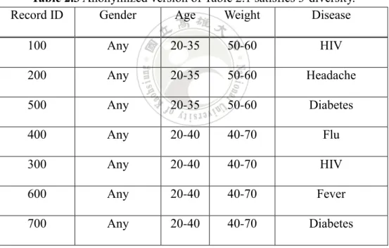
The most famous model for preserving attribute disclosure is l-diversity [11], which requires each QID group containing at least l sensitive values, ensuring the probability that the sensitive value within each QID group will be no more than 1/l. Table 2.3 shows an example anonymization of Table 2.1 satisfies 3-diversity. Due to the first group of gender fields containing both male and female, we have to generalize gender value into “Any”.

Table 2.1 Example of privacy attack of record disclosure.

(a) An example of de-identified published data

Record ID Gender Age weight Disease

100 Male 30 60 HIV 200 Male 20 50 HIV 300 Male 40 70 Diabetes 400 Female 30 40 Flu 500 Female 35 60 Headache 600 Female 38 50 Fever 700 Female 20 50 Diabetes

(b) An example of external data

Name Gender Age Zip Code

Mark Male 30 55102

Mary Female 38 53484

Lissa Female 20 51216

John Male 60 45515

Table 2.2 Anonymized version of Table 2.1 that satisfies 3-anonmity.

Record ID Gender Age Weight Disease

100 Male 20-40 50-70 HIV 200 Male 20-40 50-70 HIV 300 Male 20-40 50-70 Diabetes 400 Female 20-38 40-70 Flu 500 Female 20-38 40-70 Headache 600 Female 20-38 40-70 Fever 700 Female 20-38 40-70 Diabetes

Table 2.3 Anonymized version of Table 2.1 satisfies 3-diversity.

Record ID Gender Age Weight Disease

100 Any 20-35 50-60 HIV 200 Any 20-35 50-60 Headache 500 Any 20-35 50-60 Diabetes 400 Any 20-40 40-70 Flu 300 Any 20-40 40-70 HIV 600 Any 20-40 40-70 Fever 700 Any 20-40 40-70 Diabetes

2.2 Anonymization Methods

Since an anonymization method is designed for a specific privacy model, different privacy models must have corresponding anonymization methods. Nevertheless, these methods are mainly based on some common anonymous operations, which can be roughly divided into three categories: generalization [8], suppression, anatomization and permutation [14, 16], and random perturbation [1].

Generalization is to change the attribute value to a higher level according to a

predefined attribute taxonomy. For example, for an occupation attribute, we may change the occupation from “Painter” to “Artist”. Suppression is simply to remove an attribute or change it to a specific value. Anatomization is to divide the data into two data tables; one is composed of QID plus a group coding field (GroupID), and the other is composed of three fields: GroupID and SA and count. In this way, the correspondence between the QID attribute and the SA attribute in each QID group is rearranged. Random perturbation [1] is to add numerical or non-numeric values as noise to sensitive attributes by data swapping or synthetic data generation.

There are two types of data quality indicators for measuring the anonymized data: general indicators and specific indicators. The general indicator refers to the fact that the analyst does not know how the public information will be analyzed in the future. Therefore, the difference between the data before and after the concealment is measured by the similarity. Commonly used indices include Common Distortion (MD) [12, 13], Information Loss (IL) [15] and the Discriminant Index (DM) [3]. On the other hand, the specific index is used when the type of analysis is known to the analyst. For example, Classification Metric (CM) is used for measuring data dedicate to classification work [7].

Chapter 3 Problem Statement

In this chapter, we will describe the problem of anonymizing SRS data with missing values. To facilitate the discussion, we simplify the SRS data as a table D that consists of three groups of attributes, QID, SA and NSA. We first describe the features of typical SRS data, especially missing values. Then we present several problems of applying current approaches to anonymizing SRS data with missing values.

3.1 Characteristics of SRS Data

3.1.1 Missing Values

Missing value is a common problem in SRS data, since not all attributes of the data are mandatory to be submitted. For example, our analysis show that there are more than 70% of records in FAERS datasets not containing weight information, about 30% of records without age information, and around 6% of records missing gender information. Note all of the above attributes denote demographics of patients and are regarded as part of QID attributes. Contemporary work on privacy preserving data anonymization almost all assume QID attributes are complete. As such, current approaches usually remove all records containing missing values, which will significantly ruin the data effectiveness because in this way over 70% data have to be removed.

3.1.2 Other Features

In our past research [10], we also presented several features of SRS data that are not well considered by most anonymization approaches.

 Rare Events: In SRS data, it is very likely to observe undiscovered or new ADRs, especially for new marketing drugs. Therefore almost all methods for measuring the significance of ADRs do not emphasize too much the frequency of ADRs. For example, even if an event only occurs three times in the SRS data, the MHRA measurement [18] may also output it as a significant ADR signal. Most anonymization methods rely on generalization or suppression operation, which may ruin the existence of rare events and lead to false ADR signals or miss significant signals.

 Multiple Individual Records: A typical SRS data usually contains tracking data for each individual event, called follow-ups. These reports supplement the information of initial report and combine them into a more accurate version. Most existing PPDP models assume that each individual has only one corresponding record, e.g., k-anonymity and l-diversity. Ignoring multiple records of a single case can compromise existing privacy requirements. For example, a table that satisfies k-anonymity may contain a QID-group that composed of k records but all belonging to same individual, causing ineffective anonymization.

 Multi-valued Sensitive Attribute: A typical SRS data set, like FAERS, usually contains Drugs, PT, and indications for patients before treatment, called INI_PT. These attributes all contain more than one value, but very few PPDP models can manage these multi-valued sensitive attributes.

3.2 Problems of Current Anonymization

Approaches

Nearly no work has notices the problem of missing values to privacy data publishing. The work conducted by Hsiao [9], a former member of our lab, presented and studied four possible strategies to anonymize data with missing values.

The first strategy discards all records that contain missing values, then anonymize and publish the remaining part. This simple strategy eliminates the troublesome issue of handling missing values. However, if a dataset contains a large amount of missing values, after deleting the missing data, the published information will be very few, and its usability and analysis accuracy will be greatly reduced.

The second strategy is not to abandon or to deal with data with missing values. First, only data without missing values are undergone anonymization, then the missing data is merged with the anonymized part and finally being published together. This strategy avoids the data availability and utilization problem caused by the deletion of missing information. The drawback is that the missing data is published without any anonymization, so the assailant may infer the privacy of some victims.

The third strategy is to adopt some imputation method to fill up the missing values, then publish the whole data after anonymization. The risk of this strategy is: First the correctness of imputation will affect the quality of the data, which is further aggravated by anonymization; Second, filling the missing values makes the analyst unaware the incompleteness of the data, which may mislead the analyst's judgment and subsequent analysis.

Based on observation of the above three strategies, Hsiao presented the forth strategy [9]: Neither abandon nor fill in the missing values, but incorporate the

missing value data into the anonymization process. Two corresponding extensions of the well-known privacy methods, k-anonymity and l-diversity, were proposed, namely Closed k-anonymity and Closed l-diversity.

Definition 3.1 (Partial QID) Let Q = {A1, A2, …, Aq} be a set of QID attributes in a

given table D, where Ai, 1  i  q, denote an attribute. We call P, P  Q, as a partial

QID of D.

Definition 3.2 (Partial QID-group) Given a partial QID P in a table D, we define all

records with the same value in P as a partial QID-group.

Definition 3.3 (Closed k-anonymity) Given a dataset D, if each partial QID group of

D contains at least k records, we say this data table satisfies Closed k-anonymity,

which ensures that the maximum probability of a particular data provider’s identity is 1/k.

Definition 3.4 (Closed l-diversity) Given a table D, if each partial QID group of D

contains at least l different sensitive values, we say D satisfies Closed l-diversity, which ensures the probability of a particular sensitive value is no more than 1/l.

Two anonymization algorithms, called Closed k-anonymization and Closed

l-diversification were also proposed. Unfortunately, these approaches do not consider

other features of SRS data, including rare events, multiple individual records, and multi-valued sensitive attributes, and so are not feasible to anonymize SRS data.

On the other hand, the work conducted by Lin et al [10] proposed approaches dedicate to anonymize SRS data. They proposed a new privacy model called MS(k, 𝜃∗_{)-bounding and the corresponding anonymization algorithm, MS-bounding}

anonymization, to protect published SRS data from privacy attacks. However, the proposed approaches suppose that the SRS data is complete, overlooking the existence of large amount of missing records.

The purpose of this thesis is to deal with all the mentioned features of SRS data, including large number of missing values into the design of anonymization method for SRS data. We follow Hiao's [9] strategy, combining the missing and the complete parts, into the anonymization process to achieve the correctness, availability and reduce privacy risks of the protected data. Our proposed method will be described in the next chapter.

Chapter 4

The Proposed Privacy Model and

Algorithm

4.1 Closed MS(𝒌, 𝜽

∗

_)-bounding

In this section, we propose a new model, Closed MS(k, 𝜃∗_{)-bounding, which}

combines MS(k, 𝜃∗_{)-bounding [10] and Closed l-diversity [9] models to deal with the}

problems mentioned in Chapter 3. Suppose there is a SRS dataset D to be published, which is composed of three disjoint sets of attributes, QID, SA, NSA, i.e., D = <QID,

SA, NSA>, and 𝐷∗ _{denote the published SRS dataset after anonymization.}

Definition 4.1 (Confidence). Let q be a value in QID-group in D and s be a sensitive

value in SA. We define the probability (frequency) of guessing s by knowing q as

conf(q s)

Definition 4.2 (Confidence Bounding). Let S = {s1, s2, …, sm} be the set of all

possible sensitive values in SA and * = (

1, 2, …, m) the corresponding thresholds

of the sensitive values that specified by the data holder. That is, i denote the upper

bound to guess si in any partial QID-group, where 1  i  m, i.e.,

conf(q si)  i

Definition 4.3 (Closed MS(k, 𝜽∗_{)-bounding). Given S, the corresponding} *_{, and a}

(a) Any partial QID-group consists of at least k distinct individual (case);

(b) The confidence of any partial QID-group q having si must be no larger than

i.

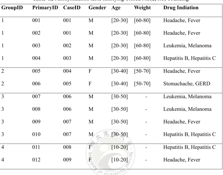
Example 4.1 Table 4.1 shows an example of an anonymized FAERS data. PrimaryID

denotes the record identifier, and CaseID the identifier of each event. A CaseID can correspond to different PrimaryIDs. Table 4.2 shows two partial QIDs {Gender, Age, Weight} and {Gender, Age, -}, where "-" indicates that the value of this attribute is missing. In terms of {Gender, Age, Weight}, there are two QID-groups, i.e., {M, [20-30], [60-80]} and {F, [30-40], [50-70]}, which are belonging to two different events. It is easy to observe that each partial QID-group contains at least two events and the frequency of each sensitive value within any partial QID-group is no more than 0.5, so this table satisfies Closed MS(2, 0.5)-bounding.

Our method will take into account missing values, but existing Information Loss index overlooks this part. So when we calculate Information Loss function, we should ignore the attributes containing missing values.

Definition 4.4 (Information loss). Assume the QID attributes can be divided into two

different sets, numerical attributes {N1, N2, …, Nm} and categorical attributes {C1,

C2, …, Cn}, where each Ci is associated with a taxonomy tree Tj. Let g denote a

QID-group. Information Loss of g is as follows:

          





where max(Ni) and min(Ni) denote the maximum and minimum values of attribute in

the whole dataset, respectively, and max(Ni, g) and min(Ni, g) denote the maximum

and minimum values of attribute in g; |g| denotes the number of records in g; h(Cj) is

the height of the taxonomy tree Tj, and h(Cj, g) is the height of the generalized value

of g intaxonomy tree Tj.

Table 4.1 An example table with missing values.

GroupID ID Age Weight Disease

1 1 45 86 Flu 1 2 36 77 Headache 1 3 - 57 Flu 2 4 30 70 Headache 2 5 40 66 Flu 2 6 10 25 Headache

For example, in Table 4.1 we can observe that ID 3 has a missing value on attribute Age. Then the Information Loss of Group 1, ignoring the missing value, will be:

IL(g) = 3 × (45−36

45−10+ 86−57

Table 4.2 Anonymization table satisfying Closed MS(2, 0.5)-bounding

GroupID PrimaryID CaseID Gender Age Weight Drug Indiation

1 001 001 M [20-30] [60-80] Headache, Fever 1 002 001 M [20-30] [60-80] Headache, Fever 1 003 002 M [20-30] [60-80] Leukemia, Melanoma 1 004 003 M [20-30] [60-80] Hepatitis B, Hepatitis C 2 005 004 F [30-40] [50-70] Headache, Fever 2 006 005 F [30-40] [50-70] Stomachache, GERD 3 007 006 M [30-50] - Leukemia, Melanoma 3 008 006 M [30-50] - Leukemia, Melanoma 3 009 007 M [30-50] - Headache, Fever 3 010 007 M [30-50] - Hepatitis B, Hepatitis C 4 011 008 F [10-20] - Hepatitis B, Hepatitis C 4 012 009 F [10-20] - Headache, Fever

4.2 Anonymization Algorithms

We propose three anonymization algorithms to meet the closed MS(k, *)-bounding model. The first one, called Closed MSpartition, adopts the concept of

partitioning dataset according to missing attributes used by algorithms closed

k-anonymization and closed l-diversification. The second one, called Closed MSdirect,

performs anonymization on the whole dataset without partition. The last one, called Closed MSsorting, employs a sorting stage before forming QID-groups. Each algorithm

will be described in each section.

4.2.1 Algorithm Closed-MS

The first algorithm, Closed-MSpartition, is a modification of MS-bounding

anonymization [10] by incorporating the partition scheme.

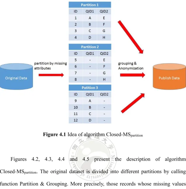
To be brief, the Closed-MSpartition algorithm first divides the input data D into

several partitions (or equivalent classes), that is, those records having missing values occurring in the same attributes are assigned to the same partition. Then we apply the same clustering approach used in MS-bounding anonymization to form QID-groups in each partition.

And finally, apply generalization for all QID-groups to anonymize the whole data. This basic idea is illustrated in Figure 4.1.

Figure 4.1 Idea of algorithm Closed-MSpartition

Figures 4.2, 4.3, 4.4 and 4.5 present the description of algorithm Closed-MSpartition. The original dataset is divided into different partitions by calling

function Partition & Grouping. More precisely, those records whose missing values exist in the same QID fields are assigned to same partition. Then, function Grouping is executed to anonymize all partitions, trying to satisfy MS(k, *)-bounding as could as possible. That is, every partial QID-group has to contain at least “k” records, and the frequency of each sensitive value in the group cannot be less than “”.

Algorithm: Closed-MSpartition

Input: The original dataset D, sensitive values S, confidence threshold 𝜃∗_{, and}

parameter k, quasi-identifier QID

Output: An anonymized dataset D* satisfying Closed_MS(k, *_)-bounding

1 G ← {}; // The set of all anonymized QID-groups

2 combine records with the same CaseID into one super record per CaseID; 3 lsD ← {}; // The set of isolated records

4 Partition&Grouping(D, QID, lsD, G, k, *); 5 D* ← Generalization(D*, lsD, k, *₎

Procedure: Partition&Grouping

Input: The original dataset D, quasi-identifier QID Output: D*, lsD

1 Let Q1, Q2, …, Qm denote the members of power set of QID;

2 // Partition D into DQ1, DQ2, … DQm

3 // (a(r) denote the value of record r in attribute a 4 for each record r in D do

5 for i = 1 to m do

6 if (a(r)  null a  Qi) and (a(r) = null a  QID – Qi) then

7 DQi ← DQi ∪ {r};

8 end if; 9 end for; 10 end for;

11 gid ← 1 //set the group id to 1 12 for each DQi, i = 1, m do 13 if |DQi| >= k then 14 D* ← D* ∪ Grouping(DQi, G, k, gid, *); 15 else 16 lsD ← lsD ∪ DQi; 17 end if; 18 end for;

Procedure: Grouping Input: D’, G, k, gid,* Output: D’, G, gid

1. r ← a randomly chosen record in D’; 2. i ← gid;

3. repeat

4. create an empty group gi into G;

5. gi ← gi  {r};

6. remove r from D’; 7. count ← 1;

8. while count < k do

9. rbest ← argminrD’ IL’(gi, r);//choose the best record in D’;

10. if | D’|< k then 11. add all records in gi into D’;

12. remove gi from G;

13. return; 14. end if

15. gi ← gi  {rbest};

16. remove rbest from D’;

17. count ← count + 1; 18. end while

19. r ← the farthest record from rbest in D’;

20. i ← i + 1; 21. until ∞

Figure 4.4 Procedure Grouping Function: Generalization

Input: D*, lsD, k, *

Output: An anonymized dataset R satisfying Closed_MS(k, *)-bounding 1. G ={𝑔₁, 𝑔₂, … … , 𝑔_𝑛} ← the set of all QID-groups in D*;

2. for each record r in lsD do

3. 𝑔𝑏𝑒𝑠𝑡← argmin𝑔∈𝐺 ΔIL’(g, r);

4. add record r to 𝑔_{𝑏𝑒𝑠𝑡}; 5. remove r from lsD;

6. end for

7. for each g ∈ G do

8. generalize non-missing QID values in g into the same QID value; 9. end for

10. D* ← all records in G; 11. return D*;

4.2.2 Algorithm Closed-MS

In this section, we present the second method Closed-MSdirect, which proceeds

without any preprocessing to anonymize the FAERS dataset, i.e., dividing the data into different partitions in accordance with missing attributes. We observed that splitting data by missing attributes may result in dissimilar records being clustered into the same QID-group causing records with missing values in different attributes losing the opportunity to be clustered together.

Figure 4.6 presents algorithmic description of algorithm Closed-MSdirect, which is

a simplified version of algorithm Closed-MSpartition. The main difference is that there

is no partitioning employed before invoking procedure Grouping. The forming of partial QID-groups is achieved by performing clustering on the whole dataset.

Algorithm: Closed-MSdirect

Input: The original dataset D, sensitive values S, confidence threshold 𝜃∗_{, and}

parameter k, quasi-identifier QID

Output: An anonymized dataset D* satisfying Closed_MS(k, *_)-bounding

1 G ← {}; // The set of all anonymized QID-groups 2 lsD ← {}; // The set of isolated records

3 combine records with the same CaseID into one super record per CaseID; 4 Grouping(D, lsD, G, k, *);

5 lsD ←D

6 D* ← Generalization(D*, lsD, k, *)

4.2.3 Algorithm Closed-MS

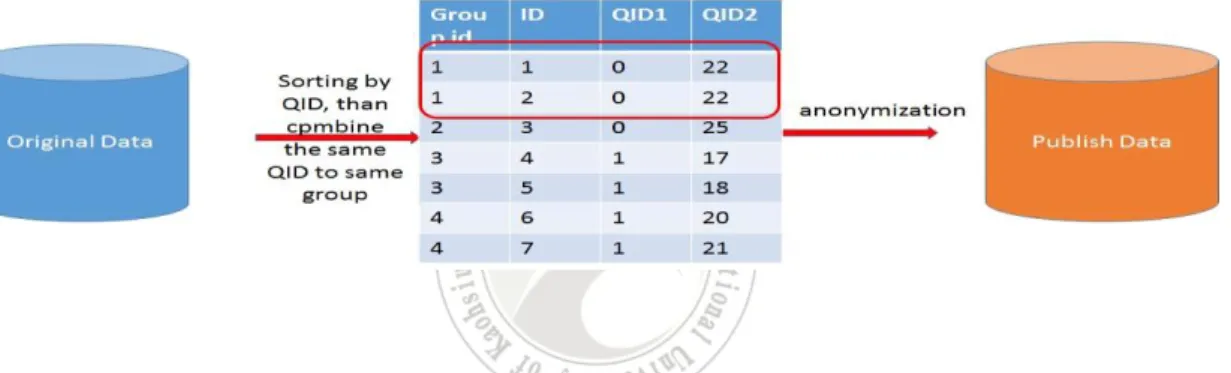
The last algorithm, we present in this section is called Closed-MSsorting. As its

name implies, we first sort data D according to QID attributes, resulting in initial groups, each composed of records with the same QID values. Then, the anonymization is performed, first generating QID-groups from the initial groups that satisfy privacy requirement. And continues by performing normal grouping to cluster the data by the similarity of records. Figure 4.7 illustrates the idea. Detailed description of Closed-MSsorting is presented in Figures 4.8 to 4.9.

Figure 4.7 Idea of algorithm Closed-MSsorting Algorithm: Closed-MSsorting

Input: The original dataset D, sensitive values S, confidence threshold 𝜃∗_{, and}

parameter k, quasi-identifier QID

Output: An anonymized dataset D* satisfying Closed MS(k, *_)-bounding

1 G ← {}; // The set of all anonymized QID-groups 2 lsD ← {}; // The records of Outlier

3 combine records with the same CaseID into one super record per CaseID; 4 Sorting&Grouping(D’, lsD, G, k, *);

5 D* ← Generalization(D*, lsD, k, *)

Procedure: Sorting&Grouping Input: D’, lsD, G, k, *

Output: D*, lsD

1 Sort the data D’ and form initial groups Q;

2 Q = {Q1, Q2, …, Qm} //Pre-grouping D’ with the same QID values into the same

QID-group; 3 gid ← 1 4 for each Qi,1≤ 𝑖 ≤ m do 5 if |𝑄_𝑖| ≥ 𝑘 and ∀ 𝑠 ∈ 𝑄_𝑖 conf(qid s)  s // 6 remove Qi from Q 7 D* ←D* ∪ Qi 8 gid ← gid +1 9 end for

10 Grouping(Qgrouped, G, k, gid ,*);

11 lsD ← Q

Chapter 5 Experiments

In this chapter, we present the experiments for evaluating the effectiveness of our methods using FAERS data. We first describe the experimental design and show the results of the experiments, then conclude our observation of the experimental results.

5.1 Experimental Design

All experiments used the data from the FAERS data set, from 2009Q1 to 2011Q4. We use {Gender, Age, Weight} as QID, CaseID as individual identifier, and INDI_PT and PT as sensitive attributes.

We compare our three methods, Closed-MSpartition, Closed-MSdirect and

Closed-MSsorting. All methods were evaluated from three aspects, including data

distortion, privacy risk, and the influence on ADR signals.

First, we consider data distortion caused by each anonymization method, which is measured by Normalized Information Loss (NIL), meaning the average information loss for each attribute of each record.

) ) ( ( | | 1 ) ( * *



where D* is an anonymized dataset, g is a QID-group, ng is the number of QID-groups

in D*_{, and |QID| is the number of attributes in QID. The range of NIL is between 0 to}

1; the larger the value, the greater the distortion of the data.

We then use Dangerous Identity Ratio (DIR) and Dangerous Sensitivity Ratio

*) ( *) ( *) ( D GroupNum D DIGNum D DIR  (5.2) *) ( *) ( *) ( D GroupNum D DSGNum D DSR  (5.3)

If the number of records in a QID-group is less than the threshold k, the QID-group is called a Dangerous Identity Group (DIG), and DIGNum(D*_{) denotes the number of}

DIG in D*_{. In a group, if any sensitive value occurs more than θ, the given}

threshold ,the group is called a Dangerous Sensitivity Group (DSG), and DSGNum(D*₎

denotes the number of DSG in D*_.

Finally the influence on ADR signals, we analyzed the signal bias for a well-known ADR rule caused by AVANDIA:

AVANDIA, Age > 18 => CEREBROVASCULAR ACCIDENT

The strength of the signal was assessed using the PRR index, which is introduced by Medical and Health Products Control Board (MHRA) to observe the relative notification ratio (PRR)[4]. The PRR is calculated as follows.

) ( ) ( PRR d c c/ b a a/    (5.4)

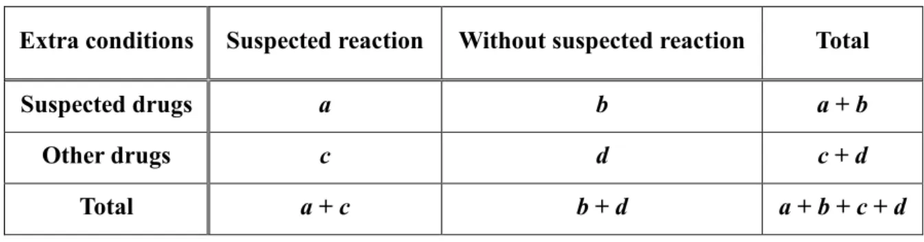
where variables a, b, c, d, are defined by the contingency table in Table 5.1, which summarizes the number of occurrences of specific drugs and adverse reactions observed in the FAERS data. Specifically, we will measure the difference of PRR for the observed ADR signal between the original data the anonymizaed data.

Table 5.1.The 22 contingency table used for the calculation of PRR.

Extra conditions Suspected reaction Without suspected reaction Total

Suspected drugs a b a + b

Other drugs c d c + d

Total a + c b + d a + b + c + d

5.2 Experimental Results

In this section, we show the results on information loss and privacy disclosure for each method. The results were performed based on two different setting of the threshold values of sensitive values, namely Confidence Setting and level-wise Confidence Setting.

5.2.1 Uniform Confidence Setting

This setting assume every symptom have the same sensitivity bounded by 0.2 or 0.4, and k = 5, 10, 15, for each anonymized group in published dataset at least k number of records.

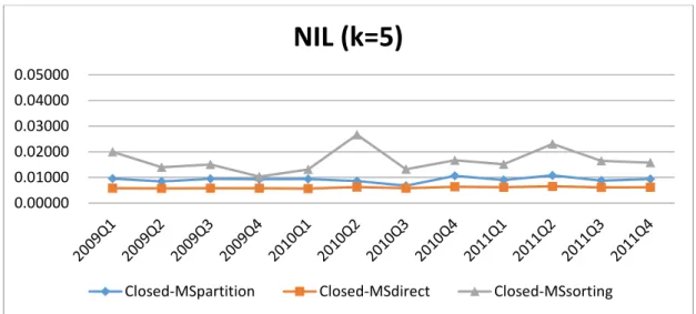
We first compare the data utility among different methods. Figures 5.1 to 5.6 show the results of NILs.

Figure 5.1. Evaluation of methods on NILs with * = 0.2 and k = 5

Figure 5.2. Evaluation of methods on NILs with * = 0.2 and k = 10

0.00000 0.01000 0.02000 0.03000 0.04000 0.05000

NIL (k=5)

Closed-MSpartition Closed-MSdirect Closed-MSsorting

0.00000 0.01000 0.02000 0.03000 0.04000 0.05000

NIL (k=10)

Figure 5.3. Evaluation of methods on NILs with * = 0.2 and k = 15

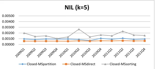
Figure 5.4. Evaluation of methods on NILs with * = 0.4 and k = 5

0.00000 0.01000 0.02000 0.03000 0.04000 0.05000

NIL (k=15)

Closed-MSpartition Closed-MSdirect Closed-MSsorting

0.00000 0.00100 0.00200 0.00300 0.00400 0.00500

NIL (k=5)

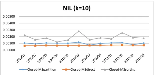
Figure 5.5. Evaluation of methods on NILs with * = 0.4 and k = 10

Figure 5.6. Evaluation of methods on NILs with * = 0.4 and k = 15

From Figures 5.1. to 5.6 we observe that

1. Closed MSdirect shows the lowest information loss among three methods, while

Closed-MSsorting above other two methods. The reason that Closed-MSsorting

exhibits the worst NILs is because the pregrouping of data was formed after sorting resulting some initial groups of a certain amount. After clustering, these groups have attract members, so that the number of QID-groups in the entire data set decreases, and the value of NIL rises.

0.00000 0.00100 0.00200 0.00300 0.00400 0.00500

NIL (k=10)

Closed-MSpartition Closed-MSdirect Closed-MSsorting

0.00000 0.00100 0.00200 0.00300 0.00400 0.00500

NIL (k=15)

2. The reason why the information loss of Closed-MSpartition is higher than

Closed-MSdirect is different from Closed-MSsorting. Closed-MSpartition divides the

data partitions in advance, then from QID-groups in each partition as much as possible, and finally the classifies remaining outlier records will be into existing groups. This may cause members in the same group that may be close in the paetition, but not necessarily in the entire dataset.

3. When 𝜃∗ _{is higher, the information loss is lower. This is because more records}

with different sensitive values must be combined to form a valid QID group, so more generalization must be performed.

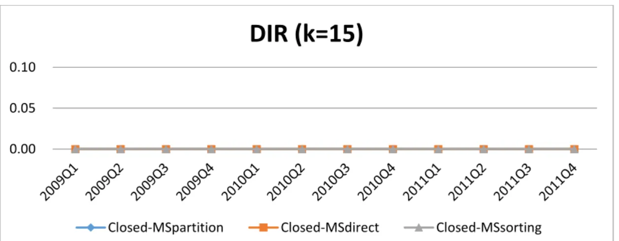
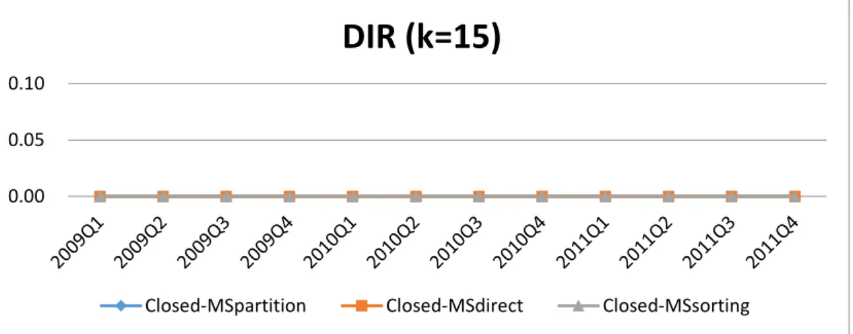
From Figures 5.7 to 5.18 we observe that

1. Regardless of all conditions, the value of DIRs is almost equal to 0, which means that each group has at least k records in all methods.

2. AS for DSRs, the differences between the three methods can be clearly observed in Figure 5.15, Closed-MSdirect incur the least DSRs and Closed-MSsorting the

worst. In Closed MSsorting, the conditionof being clustered are individual records

with the same QID values. The sensitive attributes of these records may be different, which increases the difficulty for protecting sensitive, and the privacy risk also increases.

Figure 5.7. Evaluation of methods on DIRs with * = 0.2 and k = 5

Figure 5.8. Evaluation of methods on DIRs with * = 0.2 and k = 10

Figure 5.9. Evaluation of methods on DIRs with * = 0.2 and k = 15

0.00 0.05 0.10

DIR (k=5)

Closed-MSpartition Closed-MSdirect Closed-MSsorting

0.00 0.05 0.10

DIR (k=10)

Closed-MSpartition Closed-MSdirect Closed-MSsorting

0.00 0.05 0.10

DIR (k=15)

Figure 5.10. Evaluation of methods on DIRs with * = 0.4 and k = 5

Figure 5.11. Evaluation of methods on DIRs with * = 0.4 and k = 5

Figure 5.12. Evaluation of methods on DIRs with * = 0.4 and k = 5

0.00 0.05 0.10

DIR (k=5)

Closed-MSpartition Closed-MSdirect Closed-MSsorting

0.00 0.05 0.10

DIR (k=10)

Closed-MSpartition Closed-MSdirect Closed-MSsorting

0.00 0.05 0.10

DIR (k=15)

Figure 5.13. Evaluation of methods on DSRs with * = 0.2 and k = 5

Figure 5.14. Evaluation of methods on DSRs with * = 0.2 and k = 10

Figure 5.15. Evaluation of methods on DSRs with * = 0.2 and k = 15

0.00 0.01 0.02 0.03

DSR (k=5)

Closed-MSpartition Closed-MSdirect Closed-MSsorting

0.00 0.01 0.02 0.03

DSR (k=10)

Closed-MSpartition Closed-MSdirect Closed-MSsorting

0.00 0.01 0.02 0.03

DSR (k=15)

Figure 5.16. Evaluation of methods on DSRs with * = 0.4 and k = 5

Figure 5.17. Evaluation of methods on DSRs with * = 0.4 and k = 10

Figure 5.18. Evaluation of methods on DSRs with * = 0.4 and k = 15

0.00 0.01 0.02 0.03

DSR (k=5)

Closed-MSpartition Closed-MSdirect Closed-MSsorting

0.00 0.01 0.02 0.03

DSR (k=10)

Closed-MSpartition Closed-MSdirect Closed-MSsorting

0.00 0.01 0.02 0.03

DSR (k=15)

5.2.2 Level-wise Confidence Setting

In this section, we adopted level-wise setting of * to observe the more practical situation. In the real-life case, not all symptoms are “really” sensitive. We follow our previous study in [10], choosing a group of symptoms called “Acquired immunodeficiency syndromes” (a High Level Term (HLT) in MedDRA, that contains 32 PTs and most of them are similar to AIDS) as “high sensitive” symptoms with confidence threshold = 0.2, and another two groups called “Coughing and associated symptoms” and “Allergies to foods, food additives, drugs and other chemicals,” which contain 44 PTs as “non-sensitive” symptoms with confidence threshold = 1. Those symptoms not belonging to the above groups are set the confidence thresholds to 0.4.

We compare our methods and assume the parameter k = 5, 10, 15. Figure 5.19 to 5.27 show the resulting NILs, DIRs and DSRs. From the obtained results, we observe that all NILs and DIRs generated are the same as those observed in Section 5.2.1, but

DSRs are relatively lower. The significant decline in DSRs, as observed in the

previous experiments, were improved due to the level-wise threshold.

Figure 5.19. Evaluation on NILs with level-wise confidence and k = 5

0.000 0.001 0.002 0.003 0.004 0.005

NIL (k=5)

Figure 5.20. Evaluation on NILs with level-wise confidence and k = 10

Figure 5.21. Evaluation on NILs with level-wise confidence and k = 15

0.000 0.001 0.002 0.003 0.004 0.005

NIL (k=10)

Closed-MSpartition Closed-MSdirect Closed-MSsorting

0 0.001 0.002 0.003 0.004 0.005

NIL (k=15)

Figure 5.22. Evaluation on DIRs with level-wise confidence and k = 5

Figure 5.23. Evaluation on DIRs with level-wise confidence and k = 10

Figure 5.24. Evaluation on DIRs with level-wise confidence and k = 15

0.00 0.05 0.10

DIR (k=5)

Closed-MSpartition Closed-MSdirect Closed-MSsorting

0.00 0.05 0.10

DIR (k=10)

Closed-MSpartition Closed-MSdirect Closed-MSsorting

0.00 0.05 0.10

DIR (k=15)

Figure 5.25. Evaluation on DSRs with level-wise confidence and k = 5

Figure 5.26. Evaluation on DSRs with level-wise confidence and k = 10

Figure 5.27. Evaluation on DSRs with level-wise confidence and k = 15

0.00 0.01 0.02 0.03

DSR (k=5)

Closed-MSpartition Closed-MSdirect Closed-MSsorting

0.00 0.01 0.02 0.03

DSR (k=10)

Closed-MSpartition Closed-MSdirect Closed-MSsorting

0.00 0.01 0.02 0.03

DSR (k=15)

5.3 Influence on ADR Signals

Finally, we compare the impact of each method on the utility of FAERS data. Figures 5.28 to 5.31 show the difference of PRR between the original and anonymizaed data generated by the three methods at * = 0.2, 0.4 and k = 5, 10. Right y-axis indicates the strength of orginal PRR while left-axis shows the difference of PRR. It is clear that the second method Closed-MSsorting causes a larger fluctuation on

PRR strength, which is about 0.1~-0.35, while the other two methods exhibit relatively small errors.

Figure 5.28. The difference of PRR between the original and anonymized data with

uniform confidence setting * = 0.2 and k = 5

0 5 10 15 20 25 30 -0.4 -0.35 -0.3 -0.25 -0.2 -0.15 -0.1 -0.05 0 0.05 0.1 0.15 2009Q1 2009Q2 2009Q3 2009Q4 2010Q1 2010Q2 2010Q3 2010Q4 2011Q1 2011Q2 2011Q3 2011Q4 Original Closed-MSpartition Closed-MSdirect Closed-MSsorting

Figure 5.29. The difference of PRR between the original and anonymized data with

uniform confidence setting * = 0.2 and k = 10

Figure 5.30. The difference of PRR between the original and anonymized data with

uniform confidence setting * = 0.4 and k = 5

0 5 10 15 20 25 30 -0.2 -0.15 -0.1 -0.05 0 0.05 0.1 0.15 0.2 0.25 0.3 2009Q1 2009Q2 2009Q3 2009Q4 2010Q1 2010Q2 2010Q3 2010Q4 2011Q1 2011Q2 2011Q3 2011Q4 Original Closed-MSpartition Closed-MSdirect Closed-MSsorting

0 5 10 15 20 25 30 -0.4 -0.3 -0.2 -0.1 0 0.1 0.2 2009Q1 2009Q2 2009Q3 2009Q4 2010Q1 2010Q2 2010Q3 2010Q4 2011Q1 2011Q2 2011Q3 2011Q4 Original Closed-MSpartition Closed-MSdirect Closed-MSsorting

Figure 5.31. The difference of PRR brtween the original and anonymized data with

uniform confidence setting * = 0.4 and k = 10

0 5 10 15 20 25 30 -0.2 -0.15 -0.1 -0.05 0 0.05 0.1 0.15 0.2 0.25 0.3 2009Q1 2009Q2 2009Q3 2009Q4 2010Q1 2010Q2 2010Q3 2010Q4 2011Q1 2011Q2 2011Q3 2011Q4 Original Closed-MSpartition Closed-MSdirect Closed-MSsorting

Chapter 6 Conclusions and Future

Work

6.1 Conclusions

In this thesis, we explore the problems caused by current anonymization methods that do not consider missing values, and summarize previously proposed strategies for dealing with missing values. Furthermore, the privacy model Closed MS(k,*)-bounding are proposed to solve this problem. We also present three algorithms, Closed-MSpartition, Closed-MSdirect, and Closed-MSsorting to discuss the NILs, DIRs and

DSRs for each algorithm.

To evaluate the performance of our methods, we perform several experiments with two different settings of confidence bounding, including uniform setting and level-wise setting. We observe that Closed-MSdirect has the best performance on NILs

and DSRs among the three algorithms, and Closed-MSsorting is the worst. We also

inspect performance of the proposed three methods in terms of bias on ADR signals generated from the anonymized dataset. Analogous to the above observation, Closed-MSpartition exhibits the best performance while Closed-MSsorting shows the most

error.

Overall, the performance of the three methods in both NIL and DSR is acceptable, but from the ADR signal point of view, the third method Closed-MSsorting is not

6.2 Future Work

The impact of missing values on the data is very large, especially in FAERS, which is inevitable. How to deal with such a large amount of missing values when perform data anonymization deserves further discussion. The information loss index we use to measure the quality of anonymized data is not quite precise in terms of different interpretation of missing value. Because we do not know the actual situation of missing values, we do not know how to explain the existence of missing values when calculating IL, just consider the complete part without missing values.

Another possible avenue of future study is generalization. When we generalize the records with missing and non-missing values within the same group, we ignore the missing fields, and keep them as they are. In this way, such a group may create new privacy risks, which may deserve investigation in the future.

References

[1] C.C. Aggarwal and P.S. Yu (Eds), Privacy-Preserving Data Mining: Models and

Algorithms, Springer, New York, NY, 2008.

[2] J.W. Byun, A. Kamra, E. Bertino, and N. Li, “Efficient k-anonymization using clustering techniques,” in Proceedings of the 12th International Conference on

Database Systems for Advanced Applications, 2007, pp. 188-200.

[3] R.J. Bayardo and R. Agrawal, “Data privacy through optimal k-anonymization,” in Proceedings 21st IEEE International Conference on Data Engineering, pp. 217-228, 2005.

[4] S.J. Evans, P.C. Waller, and S. Davis, “Use of proportional reporting ratios (PRRs) for signal generation from spontaneous adverse drug reaction reports,”

Pharmacoepidemiology and Drug Safety, vol. 10, pp. 483–486, 2001.

[5] B. Fung, K. Wang, R. Chen, and P. Yu, “Privacy-preserving data publishing: a survey of recent developments,” ACM Computing Surveys, vol. 42, no. 4, article no. 14, 2010.

[6] B.C.M. Fung, K. Wang, and P.S. Yu, “Anonymizing classification data for privacy preservation,” IEEE Trans. on Knowledge and Data Engineering, vol. 19, no. 5, pp. 711–725, 2007.

[7] V.S. Iyengar, “Transforming data to satisfy privacy constraints,” in Proceedings

8th ACM SIGKDD International Conference on Knowledge Discovery and Data Mining, pp. 279–288, 2002.

[8] K. LeFevre, D.J. DeWitt, and R. Ramakrishman, “Incognito: Efficient full-domain k-anonymity,” in Proceedings 24th ACM SIGMOD International

[9] M.H. Hsiao and W.Y. Lin, “Privacy-Preserving Data Publishing with Missing Values”, 2017

[10] W.Y. Lin and D.C. Yang, “On privacy-preserving publishing of spontaneous ADE reporting data,” in Proceedings of 2013 IEEE International Conference on

Bioinformatics and Biomedicine, 2013, pp. 51-53.

[11] A. Machanavajjhala, D. Kifer, J. Gehrke, and M. Venkitasubramaniam, “l-diversity: Privacy beyond k-anonymity,” ACM Trans. on Knowledge

Discovery from Data, vol. 1, no. 1, pp. 3:1–3:52, 2007.

[12] L. Sweeney, “k-anonymity: a model for protecting privacy,” International

Journal on Uncertainty, Fuzziness and Knowledge-based Systems, vol. 10, no. 5,

pp. 557–570, 2002.

[13] P. Samarati, “Protecting respondents’ identities in microdata release,” IEEE

Trans. on Knowledge and Data Engineering, vol. 13, no. 6, pp. 1010–1027,

2001.

[14] X. Xiao and Y. Tao, “Anatomy: Simple and effective privacy preservation,” in

Proceedings 32nd International Conference on Very Large Data Bases, pp. 229–

240, 2006.

[15] X. Xiao and Y. Tao, “Personalized privacy preservation,” in Proceedings 25th

ACM SIGMOD International Conference on Management of Data, pp. 229–240,

2006.

[16] Q. Zhang, N. Koudas, D. Srivastava, and T. Yu, “Aggregate query answering on anonymized tables,” in Proceedings 23rd IEEE International Conference on

Data Engineering, pp. 116–125, 2007.

[17] FDA Adverse Event Reporting System (FAERS). Available at

[18] Medicines and Healthcare Products Regulatory Agency (MHRA). Available at https://www.gov.uk/government/organisations/medicines-and-healthcare-product s- regulatory-agency