科技部補助專題研究計畫成果報告
期末報告
利用快速頻譜影像技術量測大腦谷安酸濃度分布(第 2 年)
計 畫 類 別 : 個別型計畫 計 畫 編 號 : NSC 101-2320-B-004-001-MY2 執 行 期 間 : 102 年 08 月 01 日至 103 年 07 月 31 日 執 行 單 位 : 國立政治大學應用物理研究所 計 畫 主 持 人 : 蔡尚岳 共 同 主 持 人 : 尼大衛 計畫參與人員: 碩士級-專任助理人員:王宛琦 碩士級-專任助理人員:謝宜家 碩士班研究生-兼任助理人員:蔡育儒 碩士班研究生-兼任助理人員:王煒平 碩士班研究生-兼任助理人員:紀晏如 碩士班研究生-兼任助理人員:廖志評 碩士班研究生-兼任助理人員:黃俊皓 報 告 附 件 : 出席國際會議研究心得報告及發表論文 處 理 方 式 : 1.公開資訊:本計畫可公開查詢 2.「本研究」是否已有嚴重損及公共利益之發現:否 3.「本報告」是否建議提供政府單位施政參考:否中 華 民 國 103 年 10 月 01 日
中 文 摘 要 : 谷氨酸是大腦一種重要的興奮性神經傳導物質,。在核磁共 振頻譜上,谷氨酸本身頻譜特性相當複雜,同時會跟麩醯胺 重疊;目前利用迴訊時間平均法,可以簡化谷氨酸譜線同時 減少麩醯胺的影響,對於谷氨酸定量很有用,此方法需平均 約 16 個不同迴訊時間的頻譜,因此會增加掃描時間,造成此 方法在應用上,難以配合頻譜影像,因此提出利用 8 個回訊 時間的平均法,研究結果發現效果可以跟 16 回訊時間平均法 相似;本計畫為延續 100 年度計畫,利用快速面回訊頻譜影 像技術來減少掃描時間,以建立谷氨酸分布影像及定量方 法,而本延伸計畫第一年旨在量化的探討利用傳統掃描方式 和回訊時間平均法,在大腦谷氨酸濃度定量上的準確性,為 減少掃描時間已達到掃描參數最佳化,我們比較了回訊時間 平均法(8 及 16)跟傳統短回訊時間掃描法在相同的時間下, 對於谷氨酸定量的可信度和重現性;我們量化比較的方法 為,先利用 LCModel 來比較定量時的可信度,再透過重現性 實驗,來比較兩種方法在濃度量測上的準確度,結果證實回 訊時間平均法在谷氨酸量測的重現性及穩定性上均較短回訊 時間法優良,利用 8 次回訊時間平均法,即能在量測谷氨酸 得到相似的效果;第二年則採用了 8 次回訊時間平均法,利 用矢狀切面量測大腦內側壁上不同區域的谷氨酸分布和量測 重現性及穩定性,同樣也收集了及短回訊時間法的結果,主 要針對扣帶迴以及視丘等在腦部扮演重要功能的區域,這邊 除了谷氨酸另外並針對其他五種大腦代謝物,探討這兩種方 法量測時的重現性,目前已經不同區域之結果統整完畢,報 告了中側壁上,7 個不同區域上的量測大腦代謝訊息的重現 性及穩定性。最後統整兩年收集之矢狀切面以及橫切面資 料,用以兩種切面方式收集之頻譜資料,在量測大腦代謝物 上的穩定性上的差異,以及運用代謝物濃度校正方法後是否 有差異,目前整理結果發現,不同切面方式在量測穩定性上 非常接近,量測到的代謝物濃度在校正後也非常接近,並不 會因為切面方式不同而有差異,但在迴歸分析後的灰白質代 謝物濃度,則反應出了切面之間的差別,因此利用迴歸分析 後得到的的灰白質濃度之受試者變異性,也在不同切面有差 異,此差異性並非因灰白質切割方式不同造成的,歸究主要 原因為橫切面以及矢狀切面的灰白質組織以及腦脊隨液在影 像上分布位置不同,導致回歸分析時差異 中文關鍵詞: 面回訊頻譜影像技術、谷氨酸、回訊時間頻均法、磁共振頻 譜影像、重現性 英 文 摘 要 : 英文關鍵詞:
1
科技部補助專題研究計畫成果報告
(□期中進度報告/■期末報告)
利用快速頻譜影像技術量測大腦谷氨酸濃度分布
Quantitative Mapping of the Cerebral Glutamate Concentrations Using
Fast Magnetic Resonance Spectroscopic Imaging Technique
計畫類別:■個別型計畫 □整合型計畫
計畫編號:MOST 101- 2320 -B- 004 - 001 - MY2
執行期間: 101 年 8 月 1 日至 103 年 7 月 31 日
執行機構及系所:政治大學應用物理研究所
計畫主持人:蔡尚岳
共同主持人:尼大衛
計畫參與人員:王宛琦、廖志評、黃俊皓、王瑋平、蔡育儒
本計畫除繳交成果報告外,另含下列出國報告,共 1 份:
□執行國際合作與移地研究心得報告
■出席國際學術會議心得報告
期末報告處理方式:
1. 公開方式:
■非列管計畫亦不具下列情形,立即公開查詢
□涉及專利或其他智慧財產權,□一年□二年後可公開查詢
2.「本研究」是否已有嚴重損及公共利益之發現:■否 □是
3.「本報告」是否建議提供政府單位施政參考 ■否 □是, (請列舉提
供之單位;本部不經審議,依勾選逕予轉送)
中 華 民 國 103 年 9 月 30 日
2 目錄 前言---2 研究目的---3 文獻探討---3 研究方法---5 結果與討論---8 參考文獻---15 與計畫相關著作---18 一、前言
Glutamate (1) as the most prevalent excitatory neurotransmitter in the brain plays important role in the cerebral energy metabolism. When Glu is released at glutamaterigic synapses astrocytes will convert it from extracellular space into glutamine (Gln). This process involves the consumption of energy. In addition Glu and its conjugate inhibitory neurotransmitter, gamma-amino acid (GABA), constitute over 90% type of neurons and synapse in the cerebral cortex. As a precusor of the GABA the study of glutamate metabolism plays a central role for neurologist to understand the brain energetic function.Since neurometabolic dysfunction is related to many impairments of brain the Glu alternations can be also link to many pathological states which is very useful in prognosis, diagnosis and the understanding of pathologies. 1H Magnetic Resonance Spectroscopy (MRS) is known as a non-invasive method to detect the Glu and Gln content in the brain. Even it is quite essential to identify Glu and Gln separately in order to understand the roles of Glu and Gln in brain metabolism, due to their strong overlapping property they are usually quantified as Glu plus Gln complex (Glx) in general clinical system with filed strength around 1.5T to 3T. TE-averaged (TEavg) PRESS first proposed by Hurd et.al. in 2004 (2) average spectra acquired from different TE to simplify Glu spectral shape. This will make Glu show as a single peak while minimize Gln contribution, which can be feasible at field strength as low as 3T.
There are two important issues for mapping spatial distribution of Glu using TEavg method. First is the scan time. Due to the need to collect spectra from multiple TEs scan time will be prolonged. The use of routine chemical shift imaging method will be impractical. Therefore, Proton Echo Planar Spectroscopic Imaging (PEPSI), one of the fast magnetic resonance spectroscopic imaging (MRSI) technology (3) (4) can be used to shortened the scan time. The scan time of sub minute largely for single scan largely enhance the feasibility of TE-avg PEPSI for clinical applications. The PEPSI technique has been developed for clinical MR scanners to measure 2D and 3D metabolite distributions in several minutes (5,6). We have been working on PEPSI sequence in clinical system for several year (7) and have successfully integrated it with parallel imaging to further accelerate encoding speed (5,8). Another issue is the quantification of Glu. LCModel, a commercial software package, is one of the most popular frequency domain fitting programs which have been widely applied in many facilities and in many clinical researches (9). The prior knowledge needed for LCModel also known as the “basis” includes the information about spectral shape of each metabolite to be fitted. If spectrum is acquired by special acquisition protocol or sequence such as TE-avg, corresponding basis set describing the spectral shape of each metabolite from TE-avg should be generated first for LCModel analysis. For this purpose simulation procedure should be performed. GAMMA Visual Analysis
3
(GAVA) tool which includes convenient graphic user interface with flexible development framework (10) was developed to generate basis set used in all parametric spectral analysis procedures including LCModel. 二、研究目的
Based on the previous project, we have established simulation environment for MRS experiments using GAVA software package. Through this simulation we can optimize the scan times needed for TEavg protocol by reducing the number of steps needed. The TEavg protocol can be shortened to 8-steps instead of original 16-steps. We have also established procedures to do the partial volume and relaxation correction for the quantification of metabolite concentrations. This project is aimed to build up a MRSI method to access the concentrations of Glu in the brain. The MRSI protocol will be based on PEPSI, to achieve following properties; 1) clinical acceptable acquisition time; 2) coverage for whole brain area in 2D slice; 3) better spatial resolution than conventional MRSI; 4) Feasible for multiple slice orientation; 5) ability for longitudinal and inter subject comparison.
In the 1st year of this extended project, TEavg method will be adopted to simplify the quantification complexity of Glu. We will carefully compare the reliability of spectral fitting using CRLB and reproducibility of quantification using COV between TEavg protocols and TEcon protocols. A comprehensive comparison will be done by comparing the performance of 8- steps and 16 steps TEavg PEPSI with TEcon PEPSI in the same total acquisition time.
In the 2nd year of this project, since most MRSI studies have used a single or multiple transverse slices, information of reproducibility was derived from results in transverse view. It is important to establish the reproducibility of metabolites in brain structures using sagittal PEPSI but none of these studies have focused specifically on these regions such as medial wall. The established TEavg PEPSI will be used on the measurement of Glu level for medial wall which contains key anatomical structures of the limbic system and regions involved in top-down modulatory processes. These regions play a particularly important role in a wide range of pathological conditions including psychiatric disorders and chronic pain (11,12). There is also study showing the relation of neuronal and biochemical mechanism in this area (13). Finally, we further integrate the results from 1st and 2nd year. A comparison on the performance of metabolites quantification between transverse and sagiital PEPSI was done.
三、文獻探討
Previous there are plenty of studies showing that the Glu can be a valuable marker for various diseases. For examples, cognitive impairments in schizophrenia is related to glutamatergic dysfunction. Glu plus Glutamine (Gln) levels were correlated to the overall cognitive performance in schizophrenia (14,15). Several findings showed that energy metabolism and Glu-Gln cycle may be impaired in epilepsy. Increased Glu level is found in hippocampus possibly due to the slow Glu-Gln cycle in epileptic human hippocampus (16,17). Glu have been linked to various neuro disorders diseases s (18,19). Glu response to given stimulus or drug and alcohol addiction is also of highly interest. It has been shown that long term exposure to the ethanol may lead to imbalance of in excitatory and inhibitory neurotransmitter. Therefore elevated Glu level in hippocampus was found during the first cycle of ethanol withdraw and was much more higher in third cycle. During human ethanol detoxification taking drug is able to completely block the Glu increase (20,21). For drug administration significant Glu release was found in anterior cingulate after ketamine administration
4
(22). For response to outside stimulus experiments showed that Glu level increases in anterior cingulated gyrus with pain stimulus. This information could be useful for the development of treatments for pain. (23). There were also studies showing dynamic Glu response to the visual stimulation as fMRI setup (24).
Direct measurement of Glu content is usually carried out using short-TE MRS. With sufficient prior information about the spectral shape of Glu concentration can be quantified using post quantification algorithms (25,26). To improve the efficiency and accuracy of Glu quantification at low and middle file strength such as 3T, there are a number of methods proposed by spectral editing methods. J-refocused PRESS and coherence transfer method collected spectra from two different TE (1). However the trimming for J-refocused RF is important to maintain the similar spectral shape of Glu at different TE for subtraction and the contamination of GABA at same spectral range is another issue to be solved. A similar extension of this method is Carr-Purcell selective PRESS (CPRESS) which used a Carr-Purcell pulse train with very short interpulse interval. This has been shown to maintain the structure of multiplet such as Glu, Gln over a long TE range with only T2 relaxation decay (27). The further study showed that it can be used at low filed clinical system (1.5T) (28). One potential problem is the high SAR of multiple refocus RD pulse applied which can be optimized using the design of hyper echo pulse train. Multiple quantum coherence (MQC) is another way to simplify the detection of multiplets such as Glu. MQC filter design for Glu have been proposed before (29). The pulse sequence of MQC filtering is relatively complex and the design of sequence is based on the knowledge of coupling structure of spin system involving lots of basic knowledge in the NMR category. Another way to manipulate spin system is J difference editing which usually applies additional frequency selective RF pulse between regular 180 RF pulses to edit target resonance. For Glu the Gln filter, editing pulse takes 80~100 ms long to focus on ~13 hz gap between Glu and Gln resonances (30). The main challenging is that the spectrally selective RF is usually highly focused which means the duration of RF is rather long. 2D NMR technique is another type of the spectral editing methods. No assumption about the spin systems must be made. 2D J-resolved spectroscopy is a simple realization of 2D NMR technique (31). Multiplets will then spread in the f1 axis associated with t1 with highly resolved linewidth since the signal in t1 period is T2 relaxation and not the fast T2* decay. This will reduce the overlapping of many metabolites and make the multiplet easier to be identified and quantified compared with 1D spectrum. 2D correlation spectroscopy (COSY) is a very common and basic 2D NMR technique. Detection of complicated cross peak for in vivo condition is almost impossible because the description of complicated cross peak needs very high spectral resolution, which can be only achieved by increase t1 steps leading to prolonged scan time. Another problem is the total signal intensity is distributed into 2D cross peak lading to lower SNR. Even so the COSY has been already been used for in vivo application with some modification to allow spatial localization. One example is the constant time PRESS (CT PRESS) (32) and with optimized constant time and set up for t1 period CT PRESS can be optimized to detect Glu (33). TEavg method is an alternative approach. There are several advantages of this method. First, there is no need for further sequence modification which can be directed used at clinical system with conventional PRESS sequence. Second, the increased scan time is still under acceptable range. Third, it can be used at field strength of 3T. Due to its highly achievable property in clinical system, it has soon been adopted in clinical applications (34). Previously fly back Echo Planar Spectroscopic imaging (EPSI) with in-plane resolution 1.2 cm x 1.0 cm over 16 x 10 grid has been combined with TE-avg method (35) and it has been applied for accessing Glu in tumor patients (36).
5
The ability to acquire metabolic information from multiple voxels in volume of interest covering different brain regions increases the diagnostic value of MRS significantly. In much pathology, it is desirable to measure and compare metabolic concentrations inside a lesion, near a lesion and in healthy tissue.However traditional MRSI method called chemical shift imaging (CSI) is very time-consuming compared with MRI which is not applicable for TEavg method. In contrast, PEPSI first proposed by Mansfield (3) and then realized by Posse (4), use the spatial encoding gradient during signal acquisition based on EPI sequence. The time advantage of this method originates from the fact that an entire K-space plane is sampled within a single excitation. One phase encoding step can be removed and thus the duration of a 3D spatial/spectral space can be reduced to that of a conventional 2D space. The scan time of sub minute largely for single scan largely enhance the possibility of TEavg PEPSI for clinical applications. The PEPSI technique has been developed for clinical MR scanners to measure 2D and 3D metabolite distributions in several minutes (5,6) and with high spatial resolution (37). We have been working on PEPSI sequence in clinical system for several year (7) and have successfully integrated it with parallel imaging to further accelerate encoding speed (5,8)
四、研究方法
Normal volunteers are enrolled in this study. All experiments will be performed on 3T MR system (Skyra and Trio, SIEMENS Medical Solutions, Erlangen, Germany) with a 32-channel coil array that covers the whole brain circumferentially with eight surface receive-only coils. We use the body coil for RF excitation. Before MRS acquisitions, we acquire a fast multi-slice, axial T1-weighted images using the gradient echo sequence for anatomy localization, as required for subsequent PEPSI experiments. The parameters are as followed: TR/TE/flip angle=10ms/2ms/15o, 240x240 mm2 FOV, 256x256 matrix size, 18 image slices of 3-mm thickness without gap to cover the whole brain. Routine shimming and adjustment for water suppression will be carried out automatically by the MR system.
In the 1st year, six normal subjects (2 female/ 4 males; mean age ± standard deviation (38): 22.9±2.2 years; age range: 20-25 years) participated in this study. Both TEcon PEPSI and TEavg PEPSI protocols were conducted on each subject. 2D PEPSI data are acquired from a para-axial slice at the region of interest with parameters: matrix size = 32x32, FOV = 224 to 256 mm, slice thickness = 15 mm. TEcon protocol is conducted with 16 averages at TE=35 ms and TEavg protocol is conducted with 16 steps using TE form 35 ms to 185 ms with 10 ms steps. The TEavg protocol with 8 steps will be generated from 16 steps protocols by selecting TE form 35 ms to 185 ms with 20 ms steps. In the same way, we can also generate another TEcon data set using 8 averages. Then TEavg with 8 and 16 steps and TEcon with 8 and 16 averages PEPSI data set will be compared with each other according to the acquisition time. The TR was chosen to approximate the T1 values of metabolites for optimization of the acquisition efficiency for signal-to-noise ratio (SNR). Given previously reported T1 values ranging between 1000 ms and 1500 ms at 3T, we chose TR of 1500 ms for this protocol. The scan time for TEcon PEPSI and for TEavg PEPSI is both 12.8 minutes. All subjects underwent 2 TEcon protocols and 1 TEavg protocols. A non-water suppressed (NWS) MRSI scan without pre-saturation of the water signal was acquired using a single average for automatic phase correction and calibration of metabolite concentrations. The total acquisition time for all PEPSI scans were 40 minutes. Two subjects were scanned repeatedly six times in week to month interval to evaluate the reproducibility.
6
For the 2nd year, TEavg protocol with 8 steps was adopted according to the results of 1st year. The acquisition time for 8 steps TEavg PEPSI conducted on normal subjects was 6.4 minutes. Sixteen normal volunteers (9 females/ 7 males; mean age ± standard deviation (38): 29.9±8.2 years; age range: 21-49 years) participated in this study. All subjects were scanned to evaluate the MRSI reproducibility obtained with the TE30 protocol and the TEavg protocol. Each protocol was repeated twice in the same scan session for the assessment of short-term (within-day) reproducibility without leaving the scanner. Eight subjects returned around two weeks later (interval: 9-22 days; mean ± SD: 14.6±4.2 days) to repeat the same procedure for the assessment of long-term (between-weeks) reproducibility. For psychological assessment, all participants completed the Spielberger State-Trait Anxiety Inventory and the Beck Depression Inventory (39) prior to the first scan. Before being included in the study, participants gave their informed consent to the protocol, which was approved by the Institutional Review Board of National Yang-Ming University. A 14-mm thick sagittal plane was selected to cover the medial wall in the right hemisphere. Up to eight slices of outer-volume lipid suppression were applied along the perimeter of the brain to suppress the lipid signal. To reduce the partial volume effect from cerebrospinal fluid, the MRSI plane was placed slightly away from the central line. Experimental parameters for the TE30 protocol were TR = 1.5 s, TE = 30 ms, and number of excitations (NEX) = 8. For the TEavg protocol, 8 echo steps from 35 ms to 185 ms with 20 ms increments were acquired with a TR of 1.5 s to match the scan time of the TE30 protocol. A non-water suppressed (NWS) MRSI scan without pre-saturation of the water signal was acquired using a single average for automatic phase correction and calibration of metabolite concentrations. Field shimming and a NWS scan was performed for each of the TE30 and TEavg acquisitions. The total acquisition time for all PEPSI scans were 36 minutes.
After the PEPSI scans, multi-slice sagittal T1-weighted images were collected using a gradient echo sequence (TR/TE/FA: 250ms/2.61ms/ 70 degrees; FOV: 256 x 256; MAT: 128 x 128; slice thickness: 2mm). Seven slices were collected yielding a 14 mm volume to cover the same spatial location as the PEPSI scan. These T1 images were used as anatomical reference in the following regional analysis. For best tissue segmentation quality whole-brain MPRAGE (slice thickness=1mm, TR=8.9msec, TE=2.27msec, Flip Angle= 7°, TI=1100msec, MAT =256*256, FOV =256*256) will be collected. MPRAGE will collected only once for the same subject which takes additional 6 minutes.
PEPSI data from the different coils and measurements were saved and processed individually. Standard post processing strategies including spatial and temporal filtering, phase correction and even-odd echo editing were performed for the PEPSI data as described previously. The reconstructed spectral width of the PEPSI data after even/odd echo editing was 1086 Hz with 512 complex points yielding a spectral resolution of 2.1 Hz. MRSI data from the different coils were combined after phase correction to avoid possible artifacts caused by partial phase cancelation (5). Frequency adjustment was applied to the different measurements in the TE30 dataset and the different TEs in the TEavg dataset. Finally, data from the eight measurements with constant TE and step-wise TEs were averaged separately to yield spectra for the two protocols. LCModel will be used to analyze the PEPSI data using basis of TEcon (TE=35ms), 8 steps TEavg, 16 steps TEavg. Five metabolites commonly seen in the brain including N-Acetyl Aspartate (NAA), total Creatine (tCr) including creatine and phosphocreatine, Choline (Cho), myo-Inositol (mI), Glutamate (Glu), Glutamine (Gln) and the combination of Glutamate and Glutamine (Glx) will be quantified. Water scaling will be used by collecting another PEPSI scan without water suppression. The whole quantification analysis
7
procedures can be separate in to following steps. 1) The spectroscopic analysis of TEavg and TEcon PEPSI is done by LCModel. Metabolites maps of Glu, Gln, mI, NAA, Cre and Cho were then generated using water scaling. 2) Tissue segmentation was then carried out by SPM8 or FSL on the MPRAGE images. Probability maps of GM, WM and CSF were generated. 3) We use image registration function provided by SPM8 to locate the T1 images on the MPRAGE images. Since these T1 images are in the same spatial position as PEPSI, the registration parameters can be then applied to the segmented results acquired in 2) to generate corresponding tissue probability maps for PEPSI, which is also carried out in SPM8 by re-slice function. 4) Metabolites maps generated in 1) can then be corrected according the tissue type using these tissue probability maps.
In the 1st year, metabolites were evaluated using 5 regions-of-interest (ROIs) defined by whole brain, GM from frontal and posterior regions, and WM in left and right hemisphere. All ROIs were selected in the referenced T1 images with carefully controlled size for each subject. In the 2nd year, Metabolites were evaluated in eight ROIs and included the cortex of the right medial wall (MW), the cingulate cortex (CC), the anterior CC, the middle CC, the posterior CC, the thalamus, the medial parietal lobe, and the medial occipital lobe. Each ROI was manually selected on the individual T1 images. The MW mask was defined as the largest contour of the tCr metabolite map and excluded spurious spikes at the edge of the cortex. The CC mask was adjusted according to the shape and size of the individual structure. The other masks consisted of a fixed square matrix grid. For the anterior CC, the middle CC, the posterior CC, and the thalamus the grid size was 2 x 2 voxels. For the occipital and parietal lobes the grid sizes were 3 x 3 voxels and 4 x 4 voxels, respectively. For statistical analysis, the mean and standard deviation of metabolite concentrations inside the ROIs were calculated. In addition, the Cramer-Rao Lower Bound (CRLB), as provided by LCModel, was used as the error metric for metabolite quantification. It is the lowest bound of the standard deviation of the estimated metabolite concentration and is expressed in concentration percentage. The CRLB for each metabolite is commonly used to quantify the goodness-of-fit in LCModel (40). For the calculation of concentrations we used the following thresholds to reject voxels with unsatisfactory LCModel fit: CRLB > 20% for NAA, tCr and tCho, and CRLB > 50% for mI, Glu, Gln and Glx. Evaluation of the spectral quality was based on the linewidth at full-width at half maximum (FWHM; in parts per million) and the SNR as provided by LCModel.
For the 1st year, the reliability of fitting of metabolites Glu, Gln and Glx were evaluated by directly comparing CRLB for 8, 16 steps TEavg protocols and 8, 16 averaged TEcon protocols. Within-subject reproducibility was calculated from 5 repeated scans in two subjects. Coefficient of variations (COVs) were calculated as the standard deviation divided by the mean for the five repeated measurement. For the 2nd year, the within-day and between-weeks reproducibility of the TE30 and TEavg protocols were assessed by the COV. Here, COVs were calculated as the root mean square of the standard deviation of the two measurements divided by the mean across all subjects. Subjects were excluded from the COV analysis if less than two voxels within the ROI satisfied the CRLB threshold. This typically occurred in regions where field homogeneity adjustments are challenging (prefrontal and inferior areas), in regions with broadened spectral lines leading to unsuccessful spectral fitting (anterior CC and thalamus), and for Gln in the TEavg protocol due to successful suppression. A paired t-test was used to assess spectral quality and Glu and Glx differences in spectral fitting (CRLB) for the two protocols. Inter subject variations were investigated by mean and standard deviation of metabolite concentrations from the first scan of each subject.
8
From data collected in the 1st and 2nd year, twelve healthy volunteers (7 women and 5 men), aged 20 to 26 years (mean, 22), were enrolled in the comparison of transverse and sagittal PEPSI. Here only data using TEcon protocols with 8 averages were used. For calculating metabolite concentrations, we computed the means and standard deviations (SDs) across the EPSI slice for metabolite concentrations and CRLBs within brain region. Among all voxels within brain region, less than 1% voxels are rejected for NAA, tCr, tCho, 5% to 7% voxels are rejected for mI, and 10% to 15% voxels rejected for Glx. We performed linear regression analysis on the plot of concentrations versus the normalized GM fraction (GM ratio/ (WM ratio + GM ratio)). Metabolite concentrations of GM and WM can then be extrapolated using the regression lines to 0 and 1 (41). We used the regression method to estimate the metabolite concentration of NAA, tCr, and tCho in GM and WM for each participant, orientation, and segmentation method. The inter-subject and
intra-subject COV were estimated by dividing the SD of inter- and intra- subject variance by the overall mean. We used 2-way analysis of variance (ANOVA) to examine the significance of difference of metabolite concentrations in the sagittal plane and the transverse plane, and conducted tissue segmentation, using SPM and FSL.
五、結果與討論
(1st and 2nd year) Spatial localization of (a) sagittal PEPSI experiment and (b) transverse PEPSI experiment. For transverse PEPSI, a 15 mm transverse plane was selected at the upper edge of the ventricles. For sagittal PEPSI, a 10 mm thick sagittal plane was selected to cover the medial wall in the right hemisphere. To reduce the partial volume effect from cerebrospinal fluid, the PEPSI plane was placed slightly away from the
central line. Eight OVS bands were manually placed around the brain region. For both protocols, up to eight slices of outer volume lipid suppression were applied along the perimeter of the brain to suppress the lipid signal.
9
(1st and 2nd year) Example of ROI locations for data analysis used in the 1st year (left), and 2nd year (middle and right). Four ROIs were selected for data collected in transverse PEPSI and 8 ROIs were selected in sagiital PEPSI along medial wall.
(1st year) Glu, Gln and Glx concentrations maps (upper) and corresponding CRLB maps (lower) from a subject using TEavg and TEcon protocols. TEavg protocols give homogeneous Glu maps compared to TEcon protocols. WM and GM contrast in GLu can be better resolved in TEavg protocol. Reduced CRLB can be directly seen on the CRLB maps but due to the suppression of Gln in TEavg protocol, Glu can only be resolved using TEcon protocols. On the other hand, more smooth Glx maps and reduced CRLB values can be found in TEcon protocols.
(1st year) Reproducibility of Glu, Gln and Glx assessed by intra COV shows that TEavg protocol give better reproducibility in Glu but worse reproducibility in Gln than TEcon protocol. When Glx is considered, TEcon have better reproducibility. The fitting reliability assessed by the CRLB also indicated the similar conclusion
10
that better fitting reliability is found in Glu for TEavg protocol but in Glx for TEcon protocol. The finding show same tendency for five regional ROIs as shown in previous figure., Both 16 steps and 8 steps TEavg protocols give better reproducibility and fitting reliability in Glu compared to TEcon protocols collected at the same acquisition time. Further, higher intra-COV and higher CRLB in Glu for 8 steps TEavg protocol compared to 16 steps TEavg protocol are found. The difference is less than 3% for intra-COV and 4% for CRLB for all regional ROIs. The small difference indicated that the 8steps TEavg protocol can have similar Glu editing effect as 16 steps TEavg protocols. These results verified what we find in simulation that Glu can be individually identified using both TEavg protocols. The inert-subject variation (inter-VAR) were also calculated.
Whole brain Right hemisphere WM Left hemisphere WM
Intra-COV (%) TEavg16 TEavg8 TEcon16 TEcon8 TEavg16 TEavg8 TEcon16 TEcon8 TEavg16 TEavg8 TEcon16 TEcon8
Glu 2.42 2.36 5.44 3.59 5.78 9.80 8.69 11.43 6.00 7.80 11.89 9.70 Gln 7.91 9.18 2.93 2.34 22.28 19.62 4.89 5.59 11.25 13.11 5.31 4.69 Glx 3.44 2.10 2.32 1.58 7.11 11.21 5.20 5.55 8.51 8.54 5.09 5.74
Inter-VAR(%) TEavg16 TEavg8 TEcon16 TEcon8 TEavg16 TEavg8 TEcon16 TEcon8 TEavg16 TEavg8 TEcon16 TEcon8
Glu 7.68 7.65 2.53 17.86 3.86 7.82 11.47 15.52 4.83 14.53 0.46 16.21 Gln 12.21 7.85 2.15 27.70 24.31 16.83 8.85 38.41 20.82 24.41 2.29 31.99 Glx 8.01 7.35 1.21 9.81 7.77 7.87 9.17 16.50 11.85 16.27 0.83 10.54
CRLB(%) TEavg16 TEavg8 TEcon16 TEcon8 TEavg16 TEavg8 TEcon16 TEcon8 TEavg16 TEavg8 TEcon16 TEcon8
Glu 12.55 16.00 21.05 19.56 11.31 14.65 20.67 19.57 11.60 16.29 24.10 18.97 Gln 30.67 31.86 13.08 24.93 30.37 33.91 12.62 25.07 28.75 37.13 13.51 24.03 Glx 12.79 15.43 11.05 14.90 11.32 13.77 10.34 13.93 11.71 15.78 11.30 13.61
Frontal GM Posterior GM GM
Intra-COV(%) TEavg16 TEavg8 TEcon16 TEcon8 TEavg16 TEavg8 TEcon16 TEcon8 TEavg16 TEavg8 TEcon16 TEcon8
Glu 5.06 3.36 4.87 7.75 5.66 7.11 10.30 6.47 8.03 11.11 15.20 19.30 Gln 9.29 16.15 4.91 2.51 14.45 14.59 4.04 3.98 24.60 27.13 9.85 11.36 Glx 5.44 7.46 2.53 3.24 7.28 7.37 5.59 2.28 9.05 10.74 8.32 9.26
Inter-COV(%) TEavg16 TEavg8 TEcon16 TEcon8 TEavg16 TEavg8 TEcon16 TEcon8 TEavg16 TEavg8 TEcon16 TEcon8
Glu 9.11 15.54 13.12 25.01 8.86 8.20 5.61 22.54 16.13 18.76 7.26 19.71 Gln 29.22 25.06 0.07 24.07 24.79 16.42 2.10 37.68 38.97 36.11 8.85 34.42 Glx 11.98 18.76 5.89 13.33 13.23 9.59 2.94 16.18 12.84 8.83 7.82 10.55
CRLB(%) TEavg16 TEavg8 TEcon16 TEcon8 TEavg16 TEavg8 TEcon16 TEcon8 TEavg16 TEavg8 TEcon16 TEcon8
Glu 13.08 16.36 21.59 20.71 10.36 14.47 21.19 18.82 10.78 13.98 26.65 19.50 Gln 34.84 32.28 13.94 26.31 29.68 29.27 12.59 26.88 24.26 25.38 14.50 24.76 Glx 13.22 15.22 11.29 15.83 10.65 13.12 10.64 15.41 10.76 13.27 12.70 13.67
11
extinction, and possible spatial distortions, the NWS signal distribution and spectral quality distributions were inspected. In the figure, signal distribution and spectral quality of the non-water-suppressed (NWS) proton spectra from a representative subject. (Upper left) The anatomical (T1) reference image with the boundary of the NWS image (upper right) delineated in red. (Upper right) The NWS image was obtained by integration of the non-suppressed water peak (brighter color corresponds to higher intensity). Spectral quality was evaluated by the linewidth (lower left) and the SNR (lower right) of the water peak. The SNR was calculated as the ratio between the integrated water peak and the baseline noise. The outer contour of the water-signal distribution was found to match the anatomical image. NWS signal extinction was not observed in the ventral prefrontal region. However, broadened linewidths and poor SNRs were found in this region as well as in the brain stem and to some extend in the occipital cortex. These effects are most likely due to shimming (field homogeneity) issues and partial volume effects and agree with the variation in the anatomical structure. The SNR map did not reveal a systematic bias towards surface regions, e.g. the thalamic SNR was of similar magnitude as the cingulate SNRs. This suggests that the enhanced coil sensitivity near the brain surface observed with phased array detection may have little influence on our results.
(2nd year) Interpolated metabolite maps from the right medial wall and the matched uninterpolated CRLB maps from the first scans are shown for a representative subject. Interpolated metabolite concentration maps (in I.U.) from the right medial wall and the matched uninterpolated CRLB maps (in percent) from the first scans for a representative subject. Maps are shown for the two protocols using (a) a constant short-TE (TE30) and (b) TE-averaging (TEavg). Voxels are shown within the “medial-wall” mask. Note the different color scales for different metabolites. For TEavg, the suppression of the Gln peak and the reduction of the mI peak resulted in highly spatial non-uniform concentrations maps and increased CRLBs. Although the mean
concentrations differed between the two TE protocols they exhibited similar regional dependencies. In general, for all metabolites but tCho, the highest concentrations were found in the occipital and posterior cingulate ROIs and the lowest concentrations were found in the mid cingulate and thalamic ROIs. The relationship was opposite for tCho.
12
(2nd year) This table presents the short- (immediate within-day) and long-term (between-weeks)
reproducibility of the two protocols as assessed by the COV in the 8 ROIs. In general, the COV decreased with increasing ROI size (number of voxels). The smallest COV was obtained with the ROI covering the entire cortex of the medial wall and the largest COV was obtained in the thalamic ROI. For TE30, the COVs improved substantially in most of the ROIs when quantifying Glu and Gln together (Glx) compared to separately. Short-term reproducibility resulting from TEavg differed with respect to TE30. For the
metabolites tCr and tCho, COVs were either similar or slightly better for all ROIs using TEavg. The COVs for NAA, mI, Gln, and Glx were substantially worse for most ROIs using TEavg. Mixed results were obtained for Glu. Comparing long-term reproducibility obtained with the two TE protocols, TEavg resulted in similar or lower COVs for tCr and Glu and higher COVs for NAA, tCho, mI, Gln, and Glx. Finally, for both TE protocols the long-term paradigm mostly resulted in increased variability/ decreased reproducibility relative to the short-term paradigm. Regional reproducibility was addressed to establish the magnitude of metabolic changes to be considered significant using short- and long-term repetitive measurements.. For both short- and long-term repetitions, pairwise comparison of Glu concentrations using TEavg requires a difference of 5-8% for the large ROIs, 12-17% for the medium sized ROIs and 16-26% for the smaller cingulate ROIs. The variations obtained by TE30 for the less specific Glx were 3-5%, 8-10% and 10-15%. This finding is not surprising as Glx measured with TE30 results in better SNRs than the more specific Glu measured with TEavg. Hence, the cost of more specific metabolic information is the requirement of an increased effect size especially with increasing anatomical specificity. This comes in addition to the loss of sensitivity for other metabolites. For the three dominating metabolites in the spectrum, NAA, tCr and tCho, variations associated with long-term repetition using TE30 were between 2-10%.
13
(1st and 2nd year) Representative spectra cut out from (a) 6x6 grid of voxels in transverse PEPSI and (b) 6x6 grid of voxels in sagittal PEPSI. The location of multivoxel spectra was indicated by the box on T1 images. The spectra were shown in the range of 1 ppm to 4 ppm. Most of the spectra show typical spectral shape. Major metabolic resonance can be clearly identified on the spectra.
14
(1st and 2nd year) Mean and SD of metabolite concentrations and corresponding CRLB. Results are from sagittal PEPSI using 8 averages (SAG), transverse PEPSI using 4 averages (TRANS) and transverse PEPSI using one average (TRANS 1avg). Overall metabolite concentrations estimated from sagittal PEPSI and transverse PEPSI were at similar level. Compared with concentrations quantified without partial volume correction reported in previous studies using the same experiment parameters, concentrations with partial volume correction were 25% to 40% lower in the sagittal PEPSI and 37% to 59% lower in the transverse PEPSI (5,7,42). CRLBs of NAA, tCr and tCho were below 10%, and CRLBs of Glx were in the level of 20%. Slight lower CRLB of mI was found in sagittal PEPSI than in transverse PEPSI. Based on CRLB, the spectral quality is comparable between sagittal and transverse PEPSI. Concentrations estimated from 2 segmentation methods were at a similar level. The results showed that the transverse and sagittal EPSI have similar quantified metabolite concentrations and compatible CRLB levels over the brain region
Concentrations (mM) NAA tCr tCho mI Glx
SAG SPM 8.44±0.39 6.99±0.26 1.48±0.11 3.25±0.22 8.87±0.7 FSL 8.1±0.45 6.69±0.35 1.45±0.13 3.09±0.17 8.47±0.74 TRANS SPM 8.48±0.39 6.39±0.35 1.42±0.12 2.62±0.3 7.63±0.53 FSL 8.53±0.32 6.43±0.31 1.42±0.11 2.62±0.27 7.67±0.49 TRANS 1avg SPM 7.82±0.43 6.19±0.24 1.38±0.12 2.43±0.21 7.13±0.5 FSL 7.88±0.49 6.23±0.27 1.39±0.12 2.44±0.21 7.17±0.48
CRLB (%) NAA tCr tCho mI Glx
SAG 5.7±0.46 4.6±0.2 6.32±0.55 14.12±1.05 20.09±0.93
TRANS 5.35±0.35 4.54±0.15 6.13±0.33 17.13±1.89 20.52±1
TRANS 1avg 7.8±0.72 6.34±0.46 9.01±0.84 26.69±2.56 29.22±2.77
(1st and 2nd year) Summary of regression analysis on metabolite concentrations in GM and WM, inter-sub CV and within-sub CV. Results were from transverse PEPSI (TRANS) and sagittal PEPSI (SAG). In general, Concentrations of NAA, tCr, and tCho in GM are approximately 58%, 87%, and 25% higher than those in WM, respectively. A comparison of segmentation methods across individual data in inter-subject CV and intra-subject CV revealed that 2 segmentation routines, SPM and FSL, are consistent. There is no
statistically significant difference (P>0.1) between FSL and SPM on the estimation of concentrations of NAA, tCr and tCho in GM and WM. The estimate of NAA and tCho in WM was statistically different between the transverse PEPSI and the sagittal PEPSI (P < .01). A comparison of the sagittal PEPSI and the transverse PEPSI revealed that the inter-subject CVs of the transverse PEPSI ranged from 7% to 12% in GM and from 4% to 6% in WM. Those of the sagittal PEPSI ranged from 6% to 13% in GM and from 8% to 14% in WM. Among all metabolites, only the estimate of NAA and tCho in WM was statistically different between the transverse PEPSI and the sagittal PEPSI (P < .01). The greater variability of the sagittal PEPSI can possibly be attributed to heterogeneity of the brain structure encompassed in the sagittal plane. In
particular, the partial volume correction involving more CSF fractions, rather than 2 major components, may lead to errors during concentration estimation. The higher inter-subject CV in GM than that in WM for the transverse PEPSI can be explained by a greater CSF fraction in the proximity of the GM region. The slightly
15
reversed tendency of the inter-subject CV in GM and WM in the sagittal PEPSI can also be attributed to the spatial variability that is more confounded in the WM region than in GM in the sagittal plane. The
reproducibility of the transverse PEPSI was below 5% in GM and 4% in WM for 3 metabolites. This is in accordance with our previous report regarding transverse and sagittal PEPSI.
Concentrations (mM) Inter‐sub CV (%) Within‐sub CV (%)
GM NAA tCr tCho NAA tCr tCho NAA tCr tCho
TRANS SPM 9.97 8.22 1.60 8.21 8.45 10.80 4.65 3.90 5.02
TRANS FSL 10.21 8.49 1.65 6.81 7.48 11.50 2.68 2.23 4.15
SAG SPM 9.72 8.38 1.59 9.31 5.58 9.11
SAG FSL 10.48 8.54 1.46 9.95 7.54 12.87
WM NAA tCr tCho NAA tCr tCho NAA tCr tCho
TRANS SPM 6.81 4.35 1.20 4.51 4.84 5.89 2.46 3.67 2.20
TRANS FSL 6.85 4.39 1.20 3.89 4.02 5.61 1.19 2.65 1.79
SAG SPM 6.02 4.35 1.32 13.42 13.65 8.19
SAG FSL 5.80 4.86 1.31 12.04 10.51 9.37
In the first year, we have showed that TEavg with both 16 steps and 8 steps can be used to identify Glu individually. The fitting reliability and reproducibility is better than Econ protocols. When Glx is considered, TEcon protocols are recommended for higher signal. In the 2nd year, we established the variability of
metabolites in the medial wall of the cortex for immediate and long-term repetition of measurements. Based on this, it is possible to set the magnitude of metabolic change to be considered significant in the context of biological variability. Reproducibility was found to depend on the specific metabolite, the size of the sampled volume as well as on the anatomical location. The protocols achieved relatively low COVs with TE30 mostly showing better sensitivity than TEavg. However, while TEavg enhanced Glu and suppressed Gln, TE30 did not resolve the two metabolites. The cost of more specific glutamatergic information (Glu versus Glx) is the requirement of an increased effect size especially with increasing anatomical specificity. The protocols implemented here are reliable and may be used to study disease progression and intervention mechanisms. In addition, we have shown that quantified metabolite concentrations of sagittal and transverse EPSI, considering the partial volume effect, can be comparable and reproducible. Metabolite concentrations in GM and WM were in the reasonable range of values reported in previous studies. The associated
quantification strategy compatible with the sagittal and transverse PEPSI is feasible for quantifying metabolites concentrations.
六、參考文獻
1. Lee HK, Yaman A, Nalcioglu O. Homonuclear J-refocused spectral editing technique for quantification of glutamine and glutamate by 1H NMR spectroscopy. Magn Reson Med 1995;34(2):253-259.
2. Hurd R, Sailasuta N, Srinivasan R, Vigneron DB, Pelletier D, Nelson SJ. Measurement of brain glutamate using TE-averaged PRESS at 3T. Magn Reson Med 2004;51(3):435-440.
16
3. Mansfield P. Spatial mapping of the chemical shift in NMR. Magn Reson Med 1984;1(3):370-386. 4. Posse S, Tedeschi G, Risinger R, Ogg R, Le Bihan D. High speed 1H spectroscopic imaging in
human brain by echo planar spatial-spectral encoding. Magn Reson Med 1995;33(1):34-40.
5. Tsai SY, Otazo R, Posse S, Lin YR, Chung HW, Wald LL, Wiggins GC, Lin FH. Accelerated proton echo planar spectroscopic imaging (PEPSI) using GRAPPA with a 32-channel phased-array coil. Magn Reson Med 2008;59(5):989-998.
6. Otazo R, Tsai SY, Lin FH, Posse S. Accelerated short-TE 3D proton echo-planar spectroscopic imaging using 2D-SENSE with a 32-channel array coil. Magn Reson Med 2007;58(6):1107-1116. 7. Tsai SY, Posse S, Lin YR, Ko CW, Otazo R, Chung HW, Lin FH. Fast mapping of the T2 relaxation
time of cerebral metabolites using proton echo-planar spectroscopic imaging (PEPSI). Magn Reson Med 2007;57(5):859-865.
8. Lin FH, Tsai SY, Otazo R, Caprihan A, Wald LL, Belliveau JW, Posse S. Sensitivity-encoded (SENSE) proton echo-planar spectroscopic imaging (PEPSI) in the human brain. Magn Reson Med 2007;57(2):249-257.
9. Provencher SW. Automatic quantitation of localized in vivo 1H spectra with LCModel. NMR Biomed 2001;14(4):260-264.
10. Soher BJ, Young K, Bernstein A, Aygula Z, Maudsley AA. GAVA: spectral simulation for in vivo MRS applications. J Magn Reson 2007;185(2):291-299.
11. Colla M, Ende G, Alm B, Deuschle M, Heuser I, Kronenberg G. Cognitive MR spectroscopy of anterior cingulate cortex in ADHD: elevated choline signal correlates with slowed hit reaction times. J Psychiatr Res 2008;42(7):587-595.
12. Sudharshan N, Hanstock C, Hui B, Pyra T, Johnston W, Kalra S. Degeneration of the mid-cingulate cortex in amyotrophic lateral sclerosis detected in vivo with MR spectroscopy. AJNR Am J
Neuroradiol 2011;32(2):403-407.
13. Duncan NW, Enzi B, Wiebking C, Northoff G. Involvement of glutamate in rest-stimulus interaction between perigenual and supragenual anterior cingulate cortex: a combined fMRI-MRS study. Human brain mapping 2011;32(12):2172-2182.
14. Theberge J, Bartha R, Drost DJ, Menon RS, Malla A, Takhar J, Neufeld RW, Rogers J, Pavlosky W, Schaefer B, Densmore M, Al-Semaan Y, Williamson PC. Glutamate and glutamine measured with 4.0 T proton MRS in never-treated patients with schizophrenia and healthy volunteers. Am J Psychiatry 2002;159(11):1944-1946.
15. Theberge J, Williamson KE, Aoyama N, Drost DJ, Manchanda R, Malla AK, Northcott S, Menon RS, Neufeld RW, Rajakumar N, Pavlosky W, Densmore M, Schaefer B, Williamson PC. Longitudinal grey-matter and glutamatergic losses in first-episode schizophrenia. Br J Psychiatry
2007;191:325-334.
16. Pan JW, Williamson A, Cavus I, Hetherington HP, Zaveri H, Petroff OA, Spencer DD. Neurometabolism in human epilepsy. Epilepsia 2008;49 Suppl 3:31-41.
17. Petroff OA, Errante LD, Rothman DL, Kim JH, Spencer DD. Glutamate-glutamine cycling in the epileptic human hippocampus. Epilepsia 2002;43(7):703-710.
18. Mattson MP. Excitotoxic and excitoprotective mechanisms: abundant targets for the prevention and treatment of neurodegenerative disorders. Neuromolecular medicine 2003;3(2):65-94.
17
19. Pitt D, Werner P, Raine CS. Glutamate excitotoxicity in a model of multiple sclerosis. Nat Med 2000;6(1):67-70.
20. De Witte P. Imbalance between neuroexcitatory and neuroinhibitory amino acids causes craving for ethanol. Addictive behaviors 2004;29(7):1325-1339.
21. De Witte P, Pinto E, Ansseau M, Verbanck P. Alcohol and withdrawal: from animal research to clinical issues. Neuroscience and biobehavioral reviews 2003;27(3):189-197.
22. Rowland LM, Bustillo JR, Mullins PG, Jung RE, Lenroot R, Landgraf E, Barrow R, Yeo R, Lauriello J, Brooks WM. Effects of ketamine on anterior cingulate glutamate metabolism in healthy humans: a 4-T proton MRS study. Am J Psychiatry 2005;162(2):394-396.
23. Mullins PG, Rowland LM, Jung RE, Sibbitt WL, Jr. A novel technique to study the brain's response to pain: proton magnetic resonance spectroscopy. NeuroImage 2005;26(2):642-646.
24. Mangia S, Tkac I, Gruetter R, Van de Moortele PF, Maraviglia B, Ugurbil K. Sustained neuronal activation raises oxidative metabolism to a new steady-state level: evidence from 1H NMR spectroscopy in the human visual cortex. J Cereb Blood Flow Metab 2007;27(5):1055-1063. 25. Posse S, Otazo R, Caprihan A, Bustillo J, Chen H, Henry PG, Marjanska M, Gasparovic C, Zuo C,
Magnotta V, Mueller B, Mullins P, Renshaw P, Ugurbil K, Lim KO, Alger JR. Proton echo-planar spectroscopic imaging of J-coupled resonances in human brain at 3 and 4 Tesla. Magn Reson Med 2007;58(2):236-244.
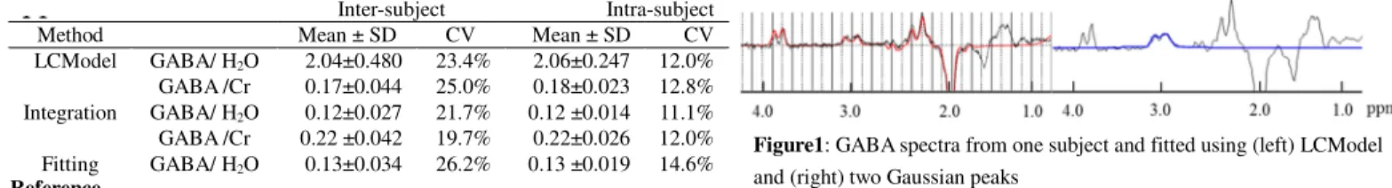
26. Henry ME, Lauriat TL, Shanahan M, Renshaw PF, Jensen JE. Accuracy and stability of measuring GABA, glutamate, and glutamine by proton magnetic resonance spectroscopy: A phantom study at 4Tesla. J Magn Reson.
27. Hennig J, Thiel T, Speck O. Improved sensitivity to overlapping multiplet signals in in vivo proton spectroscopy using a multiecho volume selective (CPRESS) experiment. Magn Reson Med
1997;37(6):816-820.
28. Soher BJ, Pattany PM, Matson GB, Maudsley AA. Observation of coupled 1H metabolite resonances at long TE. Magn Reson Med 2005;53(6):1283-1287.
29. Thompson RB, Allen PS. A new multiple quantum filter design procedure for use on strongly coupled spin systems found in vivo: its application to glutamate. Magn Reson Med
1998;39(5):762-771.
30. Choi C, Coupland NJ, Bhardwaj PP, Malykhin N, Gheorghiu D, Allen PS. Measurement of brain glutamate and glutamine by spectrally-selective refocusing at 3 Tesla. Magn Reson Med
2006;55(5):997-1005.
31. Dreher W, Leibfritz D. On the use of two-dimensional-J NMR measurements for in vivo proton MRS: measurement of homonuclear decoupled spectra without the need for short echo times. Magn Reson Med 1995;34(3):331-337.
32. Dreher W, Leibfritz D. Detection of homonuclear decoupled in vivo proton NMR spectra using constant time chemical shift encoding: CT-PRESS. Magn Reson Imaging 1999;17(1):141-150. 33. Mayer D, Spielman DM. Detection of glutamate in the human brain at 3 T using optimized constant
time point resolved spectroscopy. Magn Reson Med 2005;54(2):439-442.
34. Srinivasan R, Sailasuta N, Hurd R, Nelson S, Pelletier D. Evidence of elevated glutamate in multiple sclerosis using magnetic resonance spectroscopy at 3 T. Brain 2005;128(Pt 5):1016-1025.
18
35. Srinivasan R, Cunningham C, Chen A, Vigneron D, Hurd R, Nelson S, Pelletier D. TE-averaged two-dimensional proton spectroscopic imaging of glutamate at 3 T. NeuroImage
2006;30(4):1171-1178.
36. Li Y, Chen AP, Crane JC, Chang SM, Vigneron DB, Nelson SJ. Three-dimensional J-resolved H-1 magnetic resonance spectroscopic imaging of volunteers and patients with brain tumors at 3T. Magn Reson Med 2007;58(5):886-892.
37. Chu A, Alger JR, Moore GJ, Posse S. Proton echo-planar spectroscopic imaging with highly effective outer volume suppression using combined presaturation and spatially selective echo dephasing. Magn Reson Med 2003;49(5):817-821.
38. Ratiney H, Sdika M, Coenradie Y, Cavassila S, van Ormondt D, Graveron-Demilly D. Time-domain semi-parametric estimation based on a metabolite basis set. NMR Biomed 2005;18(1):1-13.
39. Beck AT, Ward CH, Mendelson M, Mock J, Erbaugh J. An inventory for measuring depression. Arch Gen Psychiatry 1961;4:561-571.
40. Provencher SW. Estimation of metabolite concentrations from localized in vivo proton NMR spectra. Magn Reson Med 1993;30(6):672-679.
41. Gasparovic C, Song T, Devier D, Bockholt HJ, Caprihan A, Mullins PG, Posse S, Jung RE, Morrison LA. Use of tissue water as a concentration reference for proton spectroscopic imaging. Magn Reson Med 2006;55(6):1219-1226.
42. Tsai SY, Lin YR, Wang WC, Niddam DM. Short- and long-term quantitation reproducibility of brain metabolites in the medial wall using proton echo planar spectroscopic imaging. NeuroImage
2012;63(3):1020-1029.
七、與本計畫相關著作
1. Shang-Yueh Tsai*, Woan-Chyi Wang, Yi-Ru Lin. Comparison of TE-averaged method on the
quantification of Glutamate using different steps. In preparation
2. (SCI) David M. Niddam*, Shang-Yuei Tsai, Yi-Ru Lin.Statistical mapping of metabolites in the medial wall of the brain: a proton echo planar spectroscopic imaging study. Human Brain mapping. In
revision.
3. (SCI) Shang-Yueh Tsai, Woan-Chyi Wang, Yi-Ru Lin*. Comparison of Sagittal and Transverse Echo Planar Spectroscopic Imaging on the Quantification of Brain Metabolites. Journal of Neuroimaging. 2014 Mar; published online
4. (SCI) Shang-Yuei Tsai, Yi-Ru Lin, Woan-Chyi Wang, David M. Niddam*. Short- and long-term
quantitation reproducibility of brain metabolites in the medial wall using proton echo planar spectroscopic imaging. Neuroimage. 2012 Nov;63;1020-1029.
1
科技部
補助出席國際會議報告
(補助編號:101-2320-B-004-001 –MY2 )
Joint Annual Meeting of ISMRM-ESMRMB
國際醫用磁共振學會及歐洲生醫核磁共振醫學會
共同年會
2014/05/10~2014/05/16, Milan, Italy
會議心得報告
蔡尚岳 助理教授
政治大學應用物理研究所
2 一、參加會議經過 此會議乃磁振造影界一年一度的重要會議,今年為國際醫用磁共振學會第22屆 年會於義大利米蘭舉行,因舉辦地點位於歐洲,因此與歐洲生醫磁共振醫學會31 屆年會一起舉辦,上一次共同舉辦是在2010年於瑞典斯德哥爾摩,因此不僅發表 的論文水準相當高,此年度的論文數和參予人員通常會是往年的1.5 倍左右,此 次本人共有四篇文章發表。 會議於米蘭市附近的 Convention Center 舉行,議程共分五天進行,之前再外加 兩天的 educational courses。五天內的 Scientific Meetings 總共涵蓋不同主題的 oral presentations session。每天自早上七點開始一個小時的「Sunrise educational course」,針對 MRI 各領域邀請傑出研究專家學者演講與進行座談。每天有十個 不同主題同時進行,此部分主要請一些相當有經驗的學者,已上課的形式,介紹 各領域技術的基礎和發展,雖然涵蓋很基礎的部分但是也會有很深入的探討。本 人今年主要專注於高磁場應用部分。晨間的 session 結束後接下來會議當中安排 了幾場特別的演講 (Plenary Lectures),請到領域中相當資深的研究人員主講,內 容涵蓋現今較先進之研究現況,如:Non-alcoholic fatty liver disease, Emerging
biomarker of obesity 等等,特別是禮拜一和禮拜四的 Lauterbur 以及 Mansfield
lecture, 請到 MRI 領域的資深的研究者談論目前的發展和未來,今年由 Prof. Thomas M Grist 談到 MRI 的革新,禮拜四則請到 Prof. Denis Le Bihan 教授談到 關於利用擴散性影像了解生物體微結構的部分,受益頗多。 每天大會都會安排一家磁振造影設備大廠進行最新產品的介紹,對於目前 硬體上的發展,也提供相當多資訊。而且,由於世界各地優秀研究人員均會參 加,於休息時間,像 coffee break ,亦提供了一個跟其他國家研究人員交換意見 與討論的機會。會議中參與的人士涵蓋醫界、工程界與業界。不僅可以得到工 程學術上的研究經驗,對於臨床上一些應用也更深入的瞭解 這樣的交流與學 習,不僅可以對目前頂尖 MRI 技術有更深認識,對於未來研究方向也有所助 益。
3 二、與會心得
此次會議本人延續過去研究主題,以磁振頻譜以及相關量化分析等議題
(Quantitative Methods in Musculoskeletal Tissues、Normal Brain Physiology by MRS & Other Modalities 、MRS of the CNS);擴散影像應用及技術(Diffusion: Novel Acquisition、Diffusion Tractography);fMRI 連結性相關議題(Functional
Connectivity、);肝臟相關議題(Hepatobiliary ),幫助了解目前的發展趨勢。同時 關注的還有在目前 MR 硬體技術上的發展。在一般議程中可參與晚間的研究論壇 (study group),由有興趣的研究人員共同參與討論,由資深研究人員發表實驗的一 些經驗,並由在場人員互相討論自身的使用情形,本人參與關於肝臟與肌肉脂肪 量測的議題。此外當然還有一些其他如硬體設備上的研究,以及廠商設備上的研 發現況。透過這樣的交流,使我對目前磁振造影界的發展與需求有更進一步的認 知。此行可為收穫頗豐。 三、攜回資料名稱及內容 會議論文隨身碟 四、發表論文附檔 共計發表論文四篇 僅附上論文摘要。
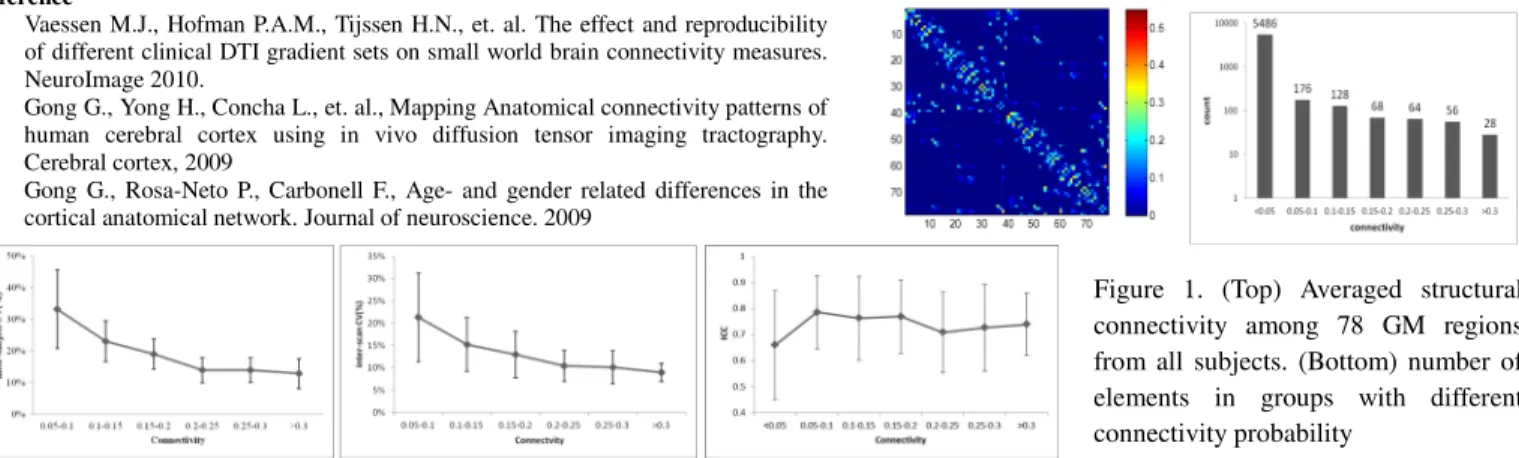
Figure 1. (Top) Averaged structural connectivity among 78 GM regions from all subjects. (Bottom) number of elements in groups with different connectivity probability
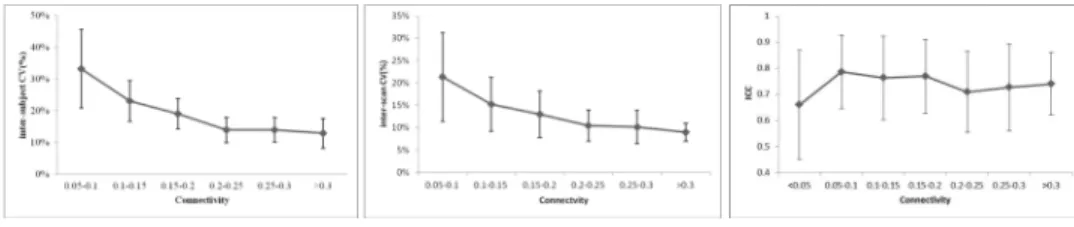
Figure 2. inter-subject CV, inter-scan CV and ICC for groups with different connectivity probability.
3274
The reproducibility of diffusion tensor imaging on brain connectivity measures between cortical regions using probabilistic tractography
Chun-Hao Huang1, Woan-Chyi Wang2, Yi-Ru Lin1, and Shang-Yueh Tsai2
1Electronic and Computer Engineering, National Taiwan University of Science and Technology, Taipei, Taiwan, 2Graduate Institute of Applied Physics, National
Chengchi University, Taipei, Taiwan
Introduction
Diffusion Tensor Imaging (DTI) associated with tractographic method has been used to investigate the structural or anatomical connectivity in the brain, which can be linked to dynamic behavior (functional connectivity) of the brain1,2. Recently, small world model in network analysis have
been widely used to study the structural networks accessed by connectivity between spatially isolated grey matter (GM) regions1,3. Although
streamline tractography has been used to track the continuity of fiber orientation along the principle diffusion tensor, the ambiguity of principle diffusion direction in GM regions make tractography strongly affected by noise1. Probabilistic tractography is an extension of streamline method that
calculates the probability of connectivity between regions with consideration of the uncertainty of major diffusion direction. Therefore, this method should be more robust and suitable for study the structural connectivity between GM regions. In this study, we investigate the test-retest reliability of structural connectivity among cortical regions parcellated in automatic anatomic labeling (AAL) template using probabilistic tractography.
Methods
Fourteen healthy subjects, 7 male and 7 female, with ages raging from 20 to 25 years old (21.8± 2.1), were recruited. Data were collected on a 3T MR system (Skyra, SIEMENS Medical Solutions, Erlangen, Germany) with a 32-channel head coil array. All subjects were scanned twice for the assessment of test-retest reproducibility. For each subject, a high-solution 3D T1 images were performed for the anatomical information. DTI protocols were performed using spin echo EPI sequence. We used 30 gradient directions with b-value 1000 s/mm2 and five additional images with
minimum diffusion weighting. Experiment parameters were TR = 8800 ms, TE = 90 ms, FOV=256x256 mm2, MAT=128x128, slice thickness = 2
mm, slice = 61, NEX = 2, acceleration factor = 2. The total acquisition time were 15 minutes including T1 and DTI scans.
The image preprocessing, estimation of diffusion parameters and tractoraphy for DTI was carried out using FSL (www.fmrib.ox.ac.uk/fsl/). Preprocessing includes motion correction, eddy current correction and brain extraction. Then we estimate the transformation matrix between standard MNI space and DTI space for each subject. A total of 78 cortical regions (39 in each hemisphere) in AAL template can be warped from MNI space into native DTI space. The local probability distribution of fiber orientation for each voxel in brain was estimated. Then probabilistic tractography was applied by sampling 5000 streamlines fibers per voxel within regions to estimate the connectivity probability between seed GM region to target GM region. Connectivity between two GM regions was displayed as number of streamlines passing target regions divided by total streamlines from seed region. Structural connectivity matrix in the order of 78 by 78 can be generated for each subject for each scan. Coefficient of variance (CV) and intra class coefficient (ICC) were calculated to characterize the inter-scan reproducibility.
Results and Discussion
Structural connectivity matrix of 78 GM regions from average of all subjects is shown in figure1. The connectivity is low between most of GM regions, which is in agreement with previous reports3. Connectivity probability among all regions is summarized by separating connectivity into
groups according to the probability. Inter-subject CV range from 33% to 13% and Inter-scan CV range from 22% to 9% for groups with connectivity strength over 0.05. Better reproducibility and less variability between subjects is found in regions with higher connectivity. For connectivity over 0.2, inter-scan CVs are at level of 10% and inter-subject CV at 13%. This implies that the DTI with probabilistic tractography can provide stable estimation on connectivity between GM regions with higher connectivity. Further, structural connectivity network of brain can be similar across subjects because network analysis is constructed majorly based on regions with higher connectivity strength. ICCs for all groups range between 0.7 to 0.8. In conclusion, we have investigated the inter-scan reproducibility of DTI on the estimation of structural connectivity between AAL cortical regions. Probabilistic tractography can be successfully applied to calculate the connectivity between GM regions at the presence of the ambiguity of principle diffusion direction in GM regions. Thus network analysis based on DTI and probabilistic tractography can be feasible.
Reference
1. Vaessen M.J., Hofman P.A.M., Tijssen H.N., et. al. The effect and reproducibility of different clinical DTI gradient sets on small world brain connectivity measures. NeuroImage 2010.
2. Gong G., Yong H., Concha L., et. al., Mapping Anatomical connectivity patterns of human cerebral cortex using in vivo diffusion tensor imaging tractography. Cerebral cortex, 2009
3. Gong G., Rosa-Neto P., Carbonell F., Age- and gender related differences in the cortical anatomical network. Journal of neuroscience. 2009
Noncontact physiological measurements using video recording inside an MRI scanner
Shang-Yi Yang1, Hsaio-Hui Huang1, Chi-Wei Liang1, Shang-Yueh Tsai2, and Teng-Yi Huang1
1National Taiwan University of Science and Technology, Taipei, Taiwan, Taiwan, 2The Graduate Institute of Applied Physics, National Chengchi University, Taipei,
Taiwan, Taiwan
Target audience: MR physicists and researchers working on correcting physiological noise. Purpose
Previous investigations showed that physiology parameters such as heart rate and respiratory rate can be measured using noncontact video recording1. This method is potentially useful in the MRI enviroment because it is an optical-based remote sensing which minmally interfers with
the fast switching MRI gradient system. However, this method requires normal ambient light as illumination source2. It is generally a low-light enviroment inside a
conventional MRI scanner. This study attempts to evaluate the feasibility of the noncontact measurement method inside the MRI enviroment and optimize the computation algorithm for MRI applications.
Methods
We performed this study in a mock MRI scanner in Taiwan Mind and Brain Imaging Center, National Chengchi University. We used a conventional digital camera (16M pixels, 4/3-inch CMOS sensor, focus length: 20mm, aperture size: F1.7) for video recording. Figure 1(a) displays the position of the camera mounted at the top of a head coil. Three volunteers participated in this experiment. During experiments, we asked the subjects to keep their heads still and recorded one minute video for each session. The video file format was 640×480 MPEG-4. During the experiment, an operator recorded the radial pulse of the volunteer’s wrist using the pads of two fingers.
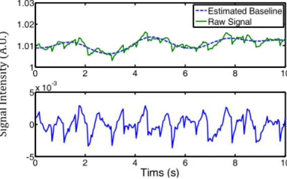
After experiments, we transferred the video files to a personal computer and performed data analysis using MATLAB® (Mathworks, Natick, MA, USA). Figure 1(c) shows the flow of image analysis. First, the three color channels, red (R), green (G) and blue (B) were separated. For each time frame, we averaged all the pixel intensities of the three images and produced three values. The procedure produced 3 signal-time curves corresponding to 3 color channels. We then used spline-based fitting to estimate the baseline drift of each curve and detrended the three curves by removing the baseline drifts from the raw signal curves. The three detrended curves underwent independent component analysis, component selection process and bass-pass filtering (0.1 - 5 Hz). Finally, we used peak detection to identify local maximum of the pulsatile curve to calculate heart rates (beats per minute) using 60 divided by time interval between two adjacent peaks.
Results
Figure 2 demonstrates the curves normalized to their initial values. Notice that the blue-channel curve fluctuates prominently. Figure 3 demonstrates the detrending procedure (top: estimating baseline drifts, bottom: the detrended curve). Figure 4 displays temporal heart-rate variations obtained from one of the volunteers.
Discussion
This study attempts to use video recording as a tool for physiology monitoring in an MRI scanner. During a cardiac cycle, facial skin blood perfusion changes alter optical path of ambient light emitted to the subject’s face. Using a conventional digital camera to capture the changes of the reflected light and using ICA analysis to remove other sources in light, we identify that this method is feasible in a low-light MRI bore. This method is an optic-based technique which avoids the problem associated with switching gradient system. This method requires off-line computation and thus is not suitable for real-time applications such as triggering cardiac imaging or cine flow measurements. Nonetheless, it is potentially useful in physiology noise corrections such as the RETROICOR method3 to remove cardiac-related noise in resting state
fMRI experiment. We performed the experiments in a mock MRI system, which is the limitation of this study. Utilizing a MRI-compatible digital camera for video recording during scans merits further investigations. In conclusion, physiology monitoring using video recording is a potential useful tool in MRI applications.
References
[1] Poh MZ, McDuff DJ, and Picard RW, “Advancements in Noncontact, Multiparameter Physiological Measurements Using a Webcam,” IEEE Trans Biomed Eng. 2011 Jan;58(1):7-11.
[2] Verkruysse W, Svaasand LO, and Nelson JS “Remote plethysmographic imaging using ambient light” Opt Express. 2008 December 22; 16(26): 21434–21445.
[3] Glover GH, Li TQ, Ress D. “Image-based method for retrospective correction of physiological motion effects in fMRI: RETROICOR.” Magn Reson Med. 2000 Jul;44(1):162-7.
Figure 1 (a) Position of the camera (b) Separating RGB color channels (c) Data analysis flow diagram
Figure 2 Normalized intensity of 3 color channels
0 5 10 15 20 25 30 35 40 45 50 0.92 0.94 0.96 0.98 1 1.02 1.04 1.06 Time (s) Norm aliz ed In tens ity (A . U .) Red Green Blue Si gn al In ten si ty ( A .U .) 0 2 4 6 8 10 1 1.01 1.02 1.03 0 2 4 6 8 10 -5 0 5 x 10 -3 Tims (s) Estimated Baseline Raw Signal
Figure 3 (top) Estimating baseline drift of the signal-time curve (bottom) the curve after baseline-drift removing 0 10 20 30 40 50 0 20 40 60 80 100 Tims (s) Hear t Rat e ( B P M )
Figure 4 An example of the obtained heart rate changes during the experiment.