國 立 交 通 大 學
機械工程學系
碩士論文
Ge-Ku-Mathieu 系統及 Sprott 19, 22 系統的
渾沌與渾沌同步
Chaos and Chaos Synchronization of Ge-Ku-Mathieu
System and Sprott 19, 22 Systems
研 究 生:王翔平
指導教授:戈正銘 教授
Ge-Ku-Mathieu 系統及 Sprott 19, 22 系統的
渾沌與渾沌同步
Chaos and Chaos Synchronization of Ge-Ku-Mathieu
System and Sprott 19, 22 Systems
研究生:王翔平 Student:
Xiang- Ping Wang指導教授:戈正銘 Advisor: Zheng-Ming Ge
國 立 交 通 大 學
機 械 工 程 學 系
碩 士 論 文
A ThesisSubmitted to Department of Mechanical Engineering College of Engineering
National Chiao Tung University In Partial Fulfillment of the Requirement
For the Degree of master of science In
Mechanical Engineering June 2010
Hsinchu, Taiwan, Republic of China
i
Ge-Ku-Mathieu 系統及 Sprott 19, 22 系統的
渾沌與渾沌同步
學生:王翔平
指導教授:戈正銘
國 立 交 通 大 學
機 械 工 程 學 系
摘要
本篇論文以相圖、龐卡萊映射圖、李亞普洛夫指數以及分歧圖等數值方法研 究新 Ge-Ku-Mathieu 系統的渾沌現象。對此系統應用部分區域穩定性理論和實用 漸進穩定理論來達成廣義同步;應用主動控制獲得雙重及多重渾沌交織同步。更 進一步使用新模糊模型來研究 Sprott 19, 22 系統的模糊模型化和渾沌同步。此 外,將探討新模糊邏輯常數控制器應用在投影同步及含有不確定性的渾沌系統。 在以上研究中,皆可由相圖和時間歷程圖得到驗證。Chaos and Chaos Synchronization of Ge-Ku-Mathieu
System and Sprott 19, 22 Systems
Student:Xiang- Ping Wang Advisor:Zheng-Ming Ge
Department of Mechanical Engineering, National Chiao Tung
University
Abstract
In this thesis, the chaotic behavior in new Ge-Ku-Mathieu system is studied by phase portraits, time history, Poincaré maps, Lyapunov exponent and bifurcation diagrams. A new kind of chaotic generalized synchronization, different translation pragmatical generalized synchronization, is obtained by pragmatical asymptotical stability theorem and partial region stability theory. Second new type for chaotic synchronization, double and multiple symplectic synchronization, are obtained by active control. A new method, using new fuzzy model, is studied for fuzzy modeling and synchronization of Sprott 19, 22 systems. Moreover, the new fuzzy logic constant controller is studied for projective synchronization and chaotic system with uncertainty. Numerical analyses, such as phase portraits and time histories can be
iii
誌謝
本篇碩士論文能夠順利的完成,首先要感謝的人,便是不斷給予耐心指導 及諄諄教誨,我的指導教授戈正銘老師。老師在我求學的過程中,在研究上,給 予我研究方向及專業領域的知識,遇到困難時,讓我學習如何克服及解決難題。 感謝老師不厭其煩的修改論文,才讓本篇論文得以完整。私底下,與老師的相處, 藉由老師深厚的文學素養,了解古今中外文史的發展,頓時對過去的史事有更深 一層的領悟。從老師的詩詞創作裡,感受到對詩詞欣賞的意境,對文學上有進一 步的認知。最後,誠摯感謝老師過去兩年辛苦的教導,對於未來的路,讓我有新 的啟發及目標。 兩年的碩士研究生涯中,感謝博士班張晉銘、李仕宇學長細心指導,碩士班 陳聰文、徐瑜韓、張育銘、陳志銘學長,在研究的過程中,給予我珍貴的意見及 鼓勵。同時要感謝同學尚恩、振賓、泳厚在課業上的幫忙以及過去的兩年中互相 扶持成長,留下許多記憶猶新的記憶。此外還要謝謝一些默默支持我的好朋友 們,無法一一列名,沒有你們就沒有我精彩的人生,在此一併感謝。 最終感謝我父親及母親對我的養育及付出,讓我得以一路順利求學,可以不 必擔心課業以外的事物,感謝弟弟們的支持。最後,感謝你們的支持,謹以此論 文獻給你們,我會勇敢堅持下去,朝理想邁進。
Contents
Chinese Abstract………..i
Abstract ………..ii
Acknowledgment……….…….iii
Contents ………iv
List of Figures ... ………vi
Chapter 1 Introduction………1
Chapter 2 Chaos for a Ge-Ku-Mathieu System……….6
2.1Preliminary………..……..6
2.2 Description of Ge-Ku-Mathieu System……….…...6
2.3 Computational Analysis of Ge-Ku-Mathieu System……….…..6
Chapter 3 Double Symplectic Synchronization for Ge-Ku-Mathieu System…...10
3.1 Preliminary………..……...10
3.2 Double Symplectic Synchronization Scheme.………..….10
3.3 Synchronization of Two Different New Chaotic Systems……….12
3.4 Summary……….……...18
Chapter 4 Different Translation Pragmatical Generalized Synchronization by Stability Theory of Partial Region for Ge-Ku-Mathieu System………...25
4.1 Preliminary……….25
4.2 The Scheme of Different Translation Pragmatic Generalized Synchronization by Stability Theory of Partial Region Theory………25
4.3 Different Translation Pragmatical Synchronization of New Ge-Ku-Mathieu Chaotic System………...……….28
4.4 Summary………37
Chapter 5 Multiple Symplectic Synchronization for Ge-Ku-Mathieu System...47
5.1 Preliminary………...47
5.2 Multiple Symplectic Synchronization Scheme.………..……....47
5.3 Synchronization of Three Different Chaotic Systems………...………...…..48
5.4 Summary………...…53
Chapter 6 Robust Projective Anti-Synchronization of Nonautonomous Chaotic S y s t e m s w i t h S t o c h a s t i c D i s t u r b a n c e b y F u z z y L o g i c C o n s t a n t Controller……….61
6.1 Preliminary………...61
6.2 Projective Chaos Anti-Synchronization by FLCC Scheme………61
6.3 Simulation Results……….65
6.4 Summary………78
v
Fuzzy Model………...92
7.1 Preliminary………92
7.2 New Fuzzy Model Theory……….………92
7.3 New Fuzzy Model of Chaotic Systems………94
7.4 Fuzzy Synchronization Scheme………103
7.5 Simulation Result………..105
7.6 Summary……….………..108
Chapter 8 Conclusions...115
Appendix A GYC Partial Region Stability Theory……….………...117
Appendix B Pragmatical Asymptotical Stability Theory……….125
List of Figures
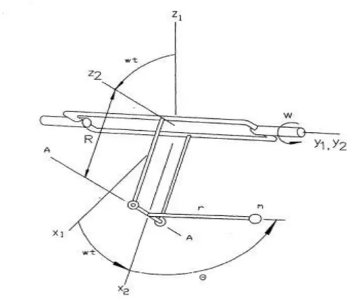
Fig. 2.1.The pendulum on rotating arm. 7
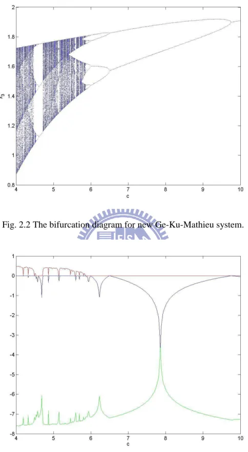
Fig. 2.2 The bifurcation diagram for new Ge-Ku-Mathieu system. 8
Fig. 2.3 The Lyapunov exponents for new Ge-Ku-Mathieu system. 8
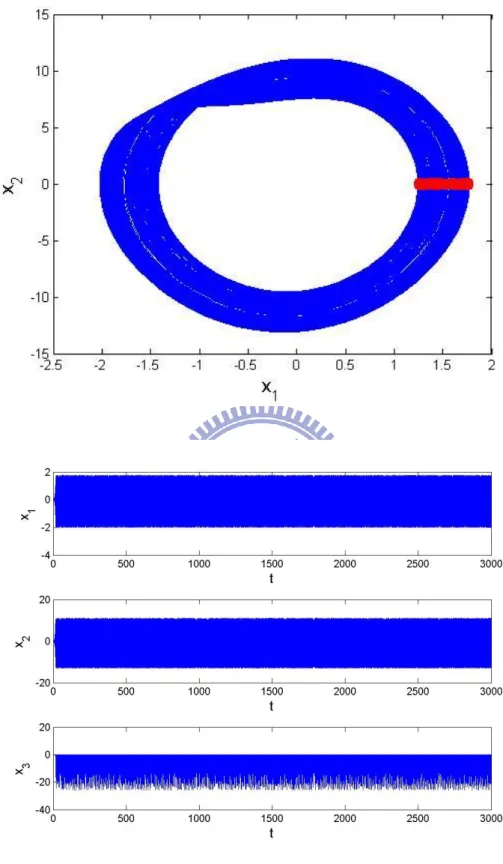
Fig. 2.4 Phase portrait, Poincaré maps, and time histories for new Ge-Ku-Mathieu system. 9
Fig. 3.1 The chaotic attractor of a new Double Ge-Ku system. 19
Fig. 3.2 The phase portrait of the controlled GKM system for Case1. 19
Fig. 3.3 Time histories of xiyi and xicosyi for Case1. 20
Fig. 3.4 Time histories of the state errors for Case1. 20
Fig. 3.5 The chaotic attractor of a new Ge-Ku-van der Pol system. 21
Fig. 3.6 The phase portrait of the controlled GKM system for Case2. 21
Fig. 3.7 Time histories of xiyi and xicosyi for Case2. 22
Fig. 3.8 Time histories of the state errors for Case2. 22
Fig. 3.9 The chaotic attractor of the Ge-Ku-Duffing system. 23
Fig. 3.10 The phase portrait of the controlled GKM system for Case3. 23
Fig. 3.11 Time histories of xiyi and xicosyi for Case3. 24
Fig. 3.12 Time histories of the state errors for Case3. 24
Fig. 4.1 Coordinate translation. 38
Fig. 4.2 Coordinate translation. 38
Fig. 4.3 Phase portrait of the error dynamic for Case 1. 39 Fig. 4.4 Time histories of x , i y for Case 1. 39 i
vii
Fig. 4.5 Time histories of errors for Case 1. 40
Fig. 4.6 Time histories of parameter errors for Case 1. 40
Fig. 4.7 Time histories of parameter errors for Case 1. 41
Fig. 4.8 Phase portrait of the error dynamic for Case 2. 41
Fig. 4.9 Time histories of x , i y for Case 2. 42 i Fig. 4.10 Time histories of errors for Case 2. 42
Fig. 4.11 Time histories of parameter errors for Case 2. 43
Fig. 4.12 Time histories of parameter errors for Case 2. 43
Fig. 4.13 Phase portrait of the error dynamic for Case 3. 44
Fig. 4.14 Time histories of x , i y for Case 3. 44 i Fig. 4.15 Time histories of errors for Case 3. 45
Fig. 4.16 Time histories of parameter errors for Case 3. 45
Fig. 4.17 Time histories of parameter errors for Case 3. 46
Fig. 5.1 The chaotic attractor of the Chen system. 54
Fig. 5.2 The chaotic attractor of the Lorenz system. 54
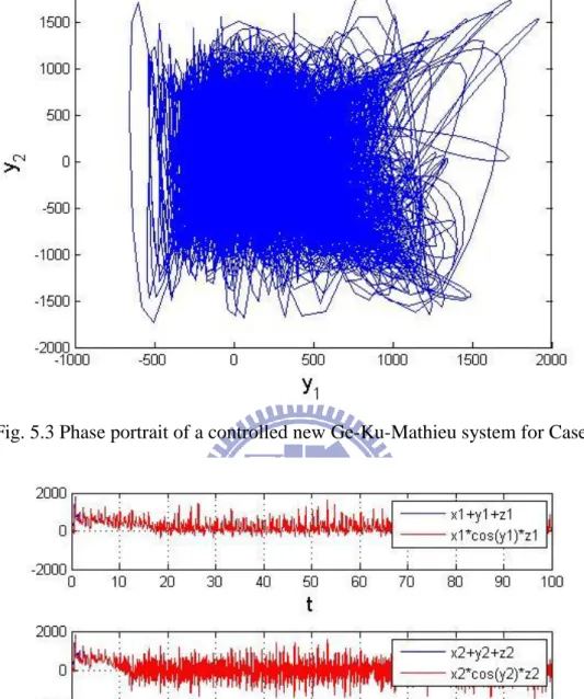
Fig. 5.3 Phase portrait of a controlled new Ge-Ku-Mathieu system for Case 1. 55
Fig. 5.4 Time histories of G( , , , )x y z t and F x y( , , , )z t for Case 1. 55
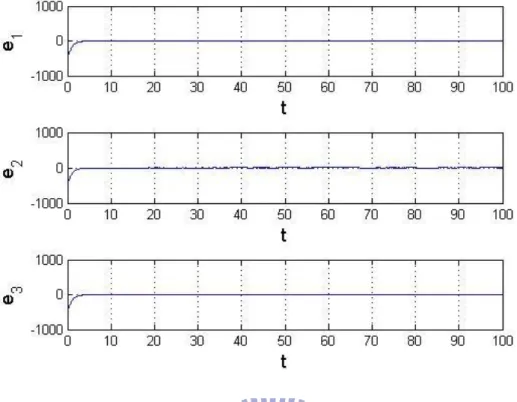
Fig. 5.5 Time histories of the state errors for Case 1. 56
Fig. 5.6 The chaotic attractor of the Rossler system. 56
Fig. 5.7 Phase portrait of the controlled Ge-Ku-Mathieu system for Case 2. 57
Fig. 5.8 Time histories of G( , , , )x y z t and F x y( , , , )z t for Case 2. 57
Fig. 5.9 Time histories of the state errors for Case 2. 58
Fig. 5.10 The chaotic attractor of the sprott system. 58
Fig. 5.12 Time histories of G( , , , )x y z t and F x y( , , , )z t for Case 3. 59
Fig. 5.13 Time histories of the state errors for Case 3. 60
Fig. 6.1. The configuration of fuzzy logic controller. 79
Fig. 6.2. Membership function. 79
Fig. 6.3. Projections of phase portrait of chaotic Sprott No.19 system with a=-0.6, b=2.75. 80
Fig. 6.4. 1 is pulse generator. 80
Fig. 6.5. Projections of phase portrait of nonautonomous chaotic Sprott 19 system and a=-0.6, b=2.75. 81
Fig. 6.6. Projections of phase portrait of chaotic Sprott 22 system with controllers. 81 Fig.6.7.Time histories of error derivatives for master and slave Sprott nonautonomous chaotic systems without controllers. 82
Fig. 6.8. Time histories of errors for Case1 (nonautonomous system) the FLCC is added after 30s. 82
Fig. 6.9. Time histories of states for Case1 (nonautonomous system) the FLCC is added after 30s. 83
Fig. 6.10. The stochastic signal of 2 is band-limited white noise(PSD=0.1). 83
Fig. 6.11. Projections of phase portrait of nonautonomous chaotic Sprott 19 system with stochastic disturbance 2, a=-0.6 and b=2.75. 84
Fig. 6.12. Time histories of error derivatives for master and slave Sprott chaotic systems without controllers. 84 Fig. 6.13. Time histories of errors for subsection 3.1.2, the FLCC is applied after 30s.
85 Fig. 6.14. Time histories of states for subsection 3.1.2, the FLCC is applied after 30s.
85 Fig. 6.15. Time histories of errors for subsection 3.1.3 the traditional nonlinear
ix
controller is applied after 30s. 86
Fig. 6.16. Time histories of states for subsection 3.1.3 the traditional nonlinear controller is applied after 30s. 86
Fig. 6.17. Projections of phase portrait of nonautonomous chaotic Sprott 19 system with stochastic disturbance where a=-0.6, b=2.75. 87
Fig. 6.18. Time histories of error derivatives for subsection 3.2.1. 87
Fig. 6.19. Time histories of errors for section 3.2 where FLCC is added after 30s. 88
Fig. 6.20. Time histories of states for subsection 2-3.2 the FLCC is coming into after 30s. 88
Fig. 6.21. Projections of phase portrait of nonautonomous chaotic Sprott 19 system with stochastic disturbance where a=-0.6, b=2.75. 89
Fig. 6.22. Time histories of error derivatives for Sprott chaotic systems without controllers. 89
Fig. 6.23. Time histories of errors for subsection 3.2.2 where FLCC are added after 30s. 90
Fig. 6.24. Time histories of states for subsection 3.2.2 where the FLCC are added after 30s. 90
Fig. 6.25. Time histories of errors for subsection 3.2.3 where the traditional controllers are added into after 30s. 91
Fig. 6.26. Time histories of states for subsection 3.2.3 where the traditional controllers are added into after 30s. 91
Fig. 7.1 Chaotic behavior of Sprott 19 system. 109
Fig. 7.2 The uncertainty signal of 1 is band-limited white noise(PSD=0.001). 109
Fig. 7.3 2 is pulse generator. 110
Fig. 7.4 Chaotic behavior of Sprott 19 system with uncertainty. 110
Fig. 7.5 Chaotic behavior of new fuzzy Sprott 19 system with uncertainty. 111
Fig. 7.7 Chaotic behavior of Sprott 22 system with uncertainty. 112
Fig. 7.8 Chaotic behavior of new fuzzy Sprott 22 system with uncertainty. 112
Fig. 7.9 Chaotic behavior of Lorenz system. 113
Fig. 7.10 Chaotic behavior of new fuzzy Lorenz system. 113
Fig. 7.11. Time histories of errors for Example 1. 114
1
Chapter 1
Introduction
Chaos is very interesting nonlinear phenomenon, exhibiting sensitive dependence on initial conditions. Because of this property, chaotic behavior is beneficial and desirable in many applications such as mixing processes, heat transfer, biological systems[1,2] , etc. Chaos synchronization is beneficial and desirable in secure communication[3,4]. Many methods of synchronization have been proposed, such as linear and nonlinear feedback control[5-11].
Generally speaking, designing a system to mimic the behavior of another chaotic system is called synchronization. Synchronization of chaotic systems has received a significant attention, since Pecora and Carroll presented the chaos synchronization method to synchronize two identical chaotic systems with different initial values in 1990 [12].
The various types of synchronization, such as complete synchronization[13], phase synchronization[14], lag synchronization[15], and generalized synchronization [16-20], are investigated extensively in the past years. Among many kinds of synchronizations, the generalized synchronization is investigated. It means there exists a functional relationship between the states of the master and those of the slave. A special kind of generalized synchronizations y x F t( ) is studied[21], where x, y are the state vectors of the master and the slave respectively, F(t) is a given vector function of time, which may take various form, either regular or chaotic functions of time. When F(t)=0, it reduces to a generalized synchronization. A new synchronization yH x y t( , , )F t( ) is studied, where x, y are the state vectors of the master and of the slave, respectively, F(t) is a given function of time in different form, such as a regular or a chaotic function. The final desired state y of the slave
system not only depends upon the master system state x but also depends upon the slave system state y itself. Therefore the slave system is not a traditional pure slave obeying the master system completely but plays a role to determine the final desired state of the slave system. In other words, it plays an interwined role, so we call this kind of synchronization is symplectic synchronization, and call the master system partner A, the slave system partner B[22].
In the current scheme of adaptive synchronization [23-27], the traditional Lyapunov stability theorem and Babalat lemma are used to prove that the error vector approaches zero, as time approaches infinity. But the question of that why the estimated parameters also approach uncertain parameters remains unanswered. By the pragmatical asymptotical stability theorem, the question can be answered strictly.
Furthermore, in chaos synchronization, most publications often assume that the synchronization system is without external disturbances. However, in practical applications, it is hard to avoid external disturbances due to uncontrollable environmental conditions. The implementation of control inputs of practical systems is frequently subject to uncertainties as a result of physical limitations. Thus, the derivation of a robust synchronization controller to resist the disturbance is studied.
In recent years, some chaos synchronizations based on fuzzy systems have been proposed since the fuzzy set theory was initiated by Zadeh [28], such as fuzzy control [29], fuzzy sliding mode controlling technique [30-31], LMI-based synchronization [32] and extended backstepping sliding mode controlling technique [33]. The fuzzy logic control (FLC) scheme has been widely developed and has been successful in many applications [34]. Recently Yau and Shieh [35] proposed a new idea in designing fuzzy logic controllers-constructing fuzzy rules subject to a common Lyapunov function such that the master-slave chaos systems satisfy stability in the Lyapunov sense. In [35], there are two main controllers in their slave system. One is
3
used in elimination of nonlinear terms and the other is built by fuzzy rules subject to a common Lyapunov function. Therefore the resulting controllers are in nonlinear form. In this paper, the regular form is necessary. In order to carry out the new method, the original system must be transformed into their regular form. Li and Ge [36] propose a new strategy which remains constructing fuzzy rules subject to Lyapunov direct method. The values of error derivatives are used to be the upper and lower bounds of FLCC. Through this new approach, a simplest constant controller can be obtained and the difficulty in realization of complicated controllers in chaos synchronization by Lyapunov direct method can be eliminated.
In recent years, fuzzy logic proposed by L. A. Zadeh [37] has received much attention as a powerful tool for the nonlinear control. Among various kinds of fuzzy methods, Takagi-Sugeno fuzzy (T-S fuzzy) system is widely accepted as a useful tool for design and analysis of fuzzy control system [38-43]. Currently, some chaos control and synchronization based on T-S fuzzy systems have been proposed, such as fuzzy sliding mode controlling technique [44-46], LMI-based synchronization [47-49] and robust control [50]. These researches are all focus on two identical nonlinear systems. Furthermore, two different nonlinear systems may have different numbers of nonlinear terms. It causes different numbers of linear subsystems. For synchronization of two different nonlinear systems, the traditional method using the idea of PDC to design the fuzzy control law for stabilization of the error dynamics can not be used here, since the number of subsystems becomes very large.
In this thesis, scheme of study is as follows. In Chapter 2, the chaos for a Ge-Ku-Mathieu (GKM) system is studied.
In Chapter 3, symplectic synchronization is defined as yH x y t( , , ), where x, y are the state vectors of the “master” and of the “slave”, respectively. The final desired state y of the “slave” not only depends upon the “master” state x but also depends
upon the “slave” state y itself. Therefore the “slave” is not a traditional pure slave obeying the “master” completely but plays a role to determine the final desired state of the “slave”system. In other words, it plays an interwined role, so we call this kind of synchronization, “symplectic synchronization”, and call the “master” system Partner A, the “slave” system Partner B. A new type of synchronization, double symplectic synchronization, G x y t( , , )F x y t( , , ) is studied, where x,y are Partner A and Partner B, respectively. Due to the complexity of the form of the double symplectic synchronization, it may be applied to increase the security of secret communication.
In Chapter 4, a new chaos synchronization strategy by different shift pragmatic synchronization by stability theory of partial region [51-52] is proposed. By using the different shift pragmatic synchronization by stability theory of partial region, the Lyapunov function is a simple linear homogeneous function of error states and the controllers are more simple and have less simulation error because they are in lower degree than that of traditional controllers, for which the Lyapunov function is a quadratic form of error states, and the question of that why the estimated parameters also approach uncertain parameters can be answered strictly.
In Chapter 5, a new type of synchronization, multiple symplectic synchronization is studied. When the double symplectic functions is extended to a more general form,
( , , ,z , , )w t ( , , ,z , , )w t
G x y F x y , it is called “multiple symplectic
synchronization”. Symplectic synchronization and double symplectic synchronization are special cases of the multiple symplectic synchronization.
In Chapter 6, the values of error derivatives are used to be the upper and lower bounds of FLCC. Through this new approach, a simplest constant controller can be obtained and the difficulty in realization of complicated controllers in chaos synchronization by Lyapunov direct method can be eliminated.
5
In Chapter 7, the new fuzzy model is proposed. It gives a new way to linearize complicated nonlinear system and only two subsystems are concluded.
Chapter 2
Chaos for a Ge-Ku-Mathieu System
2.1 Preliminary
In this Chapter, the chaotic behaviors of a new Ge-Ku Mathieu system is studied numerically by phase portraits, time histories, Poincaré maps, Lyapunov exponents, and bifurcation diagrams.
2.2 Description of Ge-Ku-Mathieu System
Ge and Ku [53] gave a chaotic system formed by a simple pendulum with its pivot rotating about a fixed axis as Fig. 2.1. This chaotic system is
1 2
2 2 1 1
,
sin [ ( cos ) sin ],
x x
x ax x b c x d wt
(2.1) where a b c d, , , are parameters. After simplification sin x1 x1 ,
2 1 1 cos 1 2 x x and addition of coupling terms, combining with Mathieu equation
3 4 3 4 3 4 3 4 4 3 , ( ) ( ) , x x x g hx x g hx nx lx px (2.2)
where g h l n p, , , , are parameters, we get the Ge-Ku-Mathieu system
1 2 2 2 2 1 1 2 3 3 1 3 2 1 3 , , , x x x ax x b c x dx x x g hx x lx px x (2.3)where a b c d g h l p, , , , , , , are parameters.
2.3 Computational Analysis of Ge-Ku-Mathieu System
For numerical analysis of computation, this system exhibits chaos when the parameters of system are a=-0.6, b=5, c=11, d=0.3, g=8, h=10, l=0.5, p=0.2 and the initial states of system are (0.01, 0.01, 0.01). The bifurcation diagram by changing damping parameter a is shown in Fig. 2.2. Its corresponding Lyapunov exponents are
7
shown in Fig. 2.3. The phase portraits, time histories, and Poincaré maps of the systems is showed in Fig. 2.4.
Fig. 2.2 The bifurcation diagram for new Ge-Ku-Mathieu system.
9
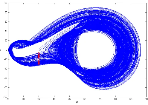
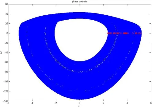
Fig. 2.4 Phase portrait, Poincaré maps, and time histories for new Ge-Ku-Mathieu system.
Chapter 3
Double Symplectic Synchronization
for Ge-Ku-Mathieu System
3.1 Preliminary
In this Chapter, a new type of synchronization, double symplectic synchronization, G x y t( , , )F x y t( , , ), for two new chaotic systems is proposed. It is an extension of symplectic synchronization, yF x y t( , , ) Since the symplectic functions are presented on both sides of the equality, it is called double symplectic synchronization. Simulations present the chaotic behaviors of two new chaotic systems. The double symplectic synchronization can be applied to the design of secure communication with more security. Finally, simulations are provided to show the effectiveness of the proposed synchronization scheme.
3.2 Double Symplectic Synchronization Scheme
Consider two different nonlinear chaotic systems, Partner A and Partner B, described by ( , )t x f x , (3.1) ( )t ( , )t y C y + g y u, (3.2) where [ ,1 2, , ]T n n x x x R x and [ ,1 2, , ]T n n y y y R
y are the state vectors of Partner A and Partner B, n n
R
C is a given matrix, f and g are continuous nonlinear vector functions, and u is the controller. Our goal is to design the controller u such that G x y( , , )t asymptotically approaches F x y( , , ),t where
( , , )t
G x y and F x y( , , )t are two given functions. For simplicity we take ( , , )t
11
Property 1 [54]: An m n matrix A of real elements defines a linear mapping yAx from R into n R , and the induced p-norm of m A for p1, 2, and is given by 1 2 T max 1 2 1 1 max , ( ) , max . m n ij ij j i i j A a A A A A a
(3.3) The useful property of induced matrix norms for real matrix A is as follow:2 1
A A A . (3.4)
Theorem: For chaotic systems “Partner A” (1) and “Partner B” (2), if the controller u is designed as 1 ( ) [ ( , ) ( ( ) ( , )) ( , ) ( , ) ( )( ) ( )], t t t t t t t y x y u I D F D Ff x D F C y g y D F f x g y C x F K x y F (3.5)
where D F , x D Fy , D F are the Jacobian matrices of t F x y( , , )t ,
1 2 diag( ,k k , ,km) K , and satisfies min( ) 1 ( ) i k t C , (3.6)
then the double symplectic synchronization will be achieved.
Proof: Define the error vectors as
( , , )t
e x y F x y , (3.7)
then the following error dynamics can be obtained by introducing the designed controller ( , ) ( ) ( , ) ( , ) ( ( ) ( , )) ( ) ( ( ) ) . t t d dt t t t t t t t x y x y y e e x y D Fx D Fy D F f x C y g y D Ff x D F C y g y D F I D F u C K e (3.8)
Choose a positive definite Lyapunov function of the form T 1 ( ) 2 V t e e. (3.9)
Taking the time derivative of V t( ) along the trajectory of Eq. (3.8), we have
T T T 2 2 2 ( ) ( ) ( ) min( ) ( ( ) min( )) . i i V t t t k t k e e e C e e Ke C e e C e (3.10)
Let ( C( )t min( ))ki e 2 M , then
2 ( ) 2 ( ) V t M e MV t . Therefore, it can be obtained that 2 ( ) (0)e Mt V t V (3.11) and 0 lim t ( )
t
V d is bounded. Besides, V t( ) is uniformly continuous.According to Barbalat’s lemma [55], the conclusion can be drawn that lim ( ) 0
tV t ,
i.e. lim ( ) 0
t e t . Thus, the double symplectic synchronization can be achieved
asymptotically.
3.3 Synchronization of Two Different New Chaotic Systems
Case 1.
Consider a new Double Ge-Ku system as Partner A described by
1 2 2 2 2 1 1 3 2 3 3 3 3 1 , , , x x x mx x n q x wx x mx x n q x rx (3.12)where m 0.5,n 1.4,q1.9,w54,r6.2 and the initial conditions are
1 2 3
13 (3.1), where
2 2 2 1 1 3 2 3 3 3 1 ( , ) x t mx x n q x wx mx x n q x rx f x . The chaotic attractor of the
Double Ge-Ku (DGK) system is shown in Fig. 3.1.
Ge-Ku-Mathieu (GKM) system is considered as Partner B. The controlled GKM system is
1 2 1 2 2 2 1 1 2 3 2 3 1 3 2 1 3 3 , , , y y u y ay y b c y dy y u y g hy y ly py y u (3.13) where a 0.6,b5,c11,d 0.3,g8,h10,l0.5,p0.2, u
u u u1, 2, 3
T is the controller, and the initial conditions are y1(0)0.01, y2(0)0.01, y3(0)0.01.Eq. (3.13) can be rewritten in the form of Eq. (3.2), where
0 1 0 ( ) 0 0 t bc a l g C and 13 1 2 3 1 3 1 3 0 ( , )t by dy y y hy y py y
g y . By applying Property 1, it is derived that
1 ( )t bc C , C( )t a bc, and C( )t 2 bc( a bc) 3058. Then ( )t 55 C is estimated. Define 1 1 2 2 3 3 cos ( , , ) cos cos x y t x y x y
F x y , and our goal is to achieve the double simplectic
synchronization x y F x y( , , )t . According to Theorem, the inequality min( ) 1 ( ) i k t
1 2 3 0 0 56 0 0 0 0 0 57 0 0 0 0 0 58 k k k
K and design the controller as
1 2cos 1 1 2sin 1 2 2 1cos 1 1 1
u x y x y y x y x y x y ,
2 2 2 2 1 1 3 2 2 2 1 1 2 3 2 2 2 2 1 1 3 2 1 1 2 3 2 2 2 2 cos sin cos , u mx x n q x wx y x ay y b c y dy y y mx x n q x wx ay y b c y dy y x y x y
2 3 3 3 3 1 3 3 1 3 2 1 3 3 2 3 3 3 1 1 3 2 1 3 3 3 3 3 cos sin cos , u mx x n q x rx y x g hy y ly py y y mx x n q x rx g hy y ly py y x y x y The Theorem is satisfied and the double symplectic synchronization is achieved, the phase portrait of the controlled GKM system is shown in Fig. 3.2. The time histories of xiyi, of xicosyi and of the state errors are shown in Fig. 3.3 and Fig. 3.4, respectively.
Case 2.
Consider a new Ge-Ku-van der Pol (GKv) system as Partner A described by
1 2 2 2 2 3 1 3 2 3 3 3 2 1 , , 1 , x x x mx x n q x wx x sx f x x rx (3.14) where m0.08,n 0.35,q100.56,w 1000.02,s0.61,f 0.08,r0.01 and the initial conditions are (0)x1 0.01, (0)x2 0.01 , (0)x3 0.01. Eq. (3.14) can berewritten in the form of Eq. (3.1), where
2 2 2 3 1 3 2 3 3 2 1 ( , ) 1 x t mx x n q x wx sx f x x rx f x .15
The chaotic attractor of a new GKv system is shown in Fig. 3.5.
A new Ge-Ku-Mathieu (GKM) system is considered as Partner B. The controlled GKM system is
1 2 1 2 2 2 1 1 2 3 2 3 1 3 2 1 3 3 , , , y y u y ay y b c y dy y u y g hy y ly py y u (3.15) where a 0.6,b5,c11,d 0.3,g8,h10,l0.5,p0.2, u
u u u1, 2, 3
T is the controller, and the initial conditions are y1(0)0.01 , y2(0)0.01 ,3(0) 0.01
y . Eq. (3.15) can be rewritten in the form of Eq. (3.2), where
0 1 0 ( ) 0 0 t bc a l g C and 13 1 2 3 1 3 1 3 0 ( , )t by dy y y hy y py y g y . By applying Property 1, it
can be derived that C( )t 1 bc , C( )t a bc , and
2 ( )t bc( a bc) 3058 C . Then C( )t 55 is estimated. Define 1 1 2 2 3 3 cos ( , , ) cos cos x y t x y x y
F x y , and our goal is to achieve the double simplectic
synchronization x y F x y( , , )t . According to Theorem, the inequality min( ) 1 ( ) i k t
C must be satisfied. It can be obtained that min( )ki 55. Thus we choose 1 2 3 0 0 56 0 0 0 0 0 57 0 0 0 0 0 58 k k k
K and design the controller as
1 2cos 1 1 2sin 1 2 2 1cos 1 1 1
2 2 2 2 3 1 3 2 2 2 1 1 2 3 2 2 2 2 3 1 3 2 1 1 2 3 2 2 2 2 cos sin cos , u mx x n q x wx y x ay y b c y dy y y mx x n q x wx ay y b c y dy y x y x y
2 3 3 3 2 1 3 3 1 3 2 1 3 3 2 3 3 2 1 1 3 2 1 3 3 3 3 3 1 cos sin 1 cos , u sx f x x rx y x g hy y ly py y y sx f x x rx g hy y ly py y x y x y The Theorem is satisfied and the double simplectic synchronization is achieved, the phase portrait of the controlled GKM system and the time histories of xiyi, of
cos
i i
x y and of the state errors are shown in Fig. 3.6 and Fig. 3.7 and Fig. 3.8, respectively.
Case 3.
Consider a new GKD system as Partner A described by
1 2 2 2 2 1 1 3 3 3 3 3 2 1 , , , x x x mx x n q x wx x x x fx rx (3.16)where m0.1,n11,q40,w54, f 6,r30 and the initial conditions are
1(0) 2, (0)2 2.4 , (0)3 5
x x x . Eq. (3.16) can be rewritten in the form of Eq. (3.1),
where
2 2 2 1 1 3 3 3 3 2 1 ( , ) x t mx x n q x wx x x fx rx f x . The chaotic attractor of the new
GKD system is shown in Fig. 3.9.
Ge-Ku-Mathieu (GKM) system is considered as Partner B. The controlled GKM system is
17
1 2 1 2 2 2 1 1 2 3 2 3 1 3 2 1 3 3 , , , y y u y ay y b c y dy y u y g hy y ly py y u (3.17) where a 0.6,b5,c11,d 0.3,g8,h10,l0.5,p0.2, u
u u u1, 2, 3
T isthe controller, and the initial conditions are y1(0)0.01, y2(0)0.01, y3(0)0.01.
Eq. (3.17) can be rewritten in the form of Eq. (3.2), where
0 1 0 ( ) 0 0 t bc a l g C and 13 1 2 3 1 3 1 3 0 ( , )t by dy y y hy y py y
g y . By applying Property 1, it can be derived that
1 ( )t bc C , C( )t a bc, and C( )t 2 bc( a bc) 3058. Then ( )t 55 C is estimated. Define 1 1 2 2 3 3 cos ( , , ) cos cos x y t x y x y
F x y , and our goal is to achieve the double simplectic
synchronization x y F x y( , , )t . According to Theorem, the inequality min( ) 1 ( ) i k t
C must be satisfied. It can be obtained that min( )ki 55. Thus we choose 1 2 3 0 0 56 0 0 0 0 0 57 0 0 0 0 0 58 k k k
K and design the controller as
1 2cos 1 1 2sin 1 2 2 1cos 1 1 1,
u x y x y y x y x y x y
2 2 2 2 1 1 3 2 2 2 1 1 2 3 2 2 2 2 1 1 3 2 1 1 2 3 2 2 2 2 cos sin cos , u mx x n q x wx y x ay y b c y dy y y mx x n q x wx ay y b c y dy y x y x y
3 3 3 3 2 1 3 3 1 3 2 1 3 3 3 3 3 2 1 1 3 2 1 3 3 3 3 3 cos sin cos , u x x fx rx y x g hy y ly py y y x x fx rx g hy y ly py y x y x y The Theorem is satisfied and the double simplectic synchronization is achieved, the phase portrait of the controlled GKM system and the time histories of xiyi, of
cos
i i
x y and of the state errors are shown in Fig. 3.10 and Fig. 3.11 and Fig. 3.12, respectively.
3.4 Summary
In this Chapter, a new double symplectic synchronization of chaotic systems are investigated based on Barbalat’s Lemma. Traditional generalized synchronization and symplectic synchronization are special cases for the double symplectic synchronization. By applying active control, the double symplectic synchronization is achieved. The simulation results show that the proposed scheme is effective and feasible for all chaotic systems. Furthermore, the double symplectic synchronization could be applied to the design of secret communication with more security than either generalized, or symplectic synchronization due to the complexity of its synchronization form.
19
Fig. 3.1 The chaotic attractor of a new Double Ge-Ku system.
Fig. 3.3 Time histories of xiyi and xicosyi for Case1.
Fig. 3.4 Time histories of the state errors for Case1.
21
Fig. 3.5 The chaotic attractor of a new Ge-Ku-van der Pol system.
Fig. 3.7 Time histories of xiyi and xicosyi for Case2.
23
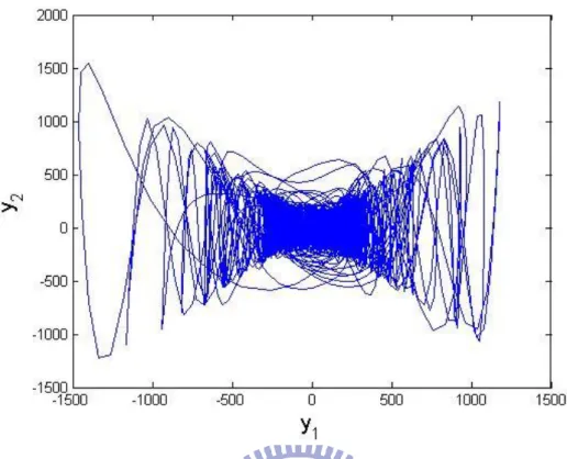
Fig. 3.9 The chaotic attractor of the Ge-Ku-Duffing system.
Fig. 3.10 The phase portrait of the controlled GKM system for Case3.
Fig. 3.11 Time histories of xiyi and xicosyi for Case3.
25
Chapter 4
Different Translation Pragmatical Generalized
Synchronization by Stability Theory of Partial Region for
Ge-Ku-Mathieu System
4.1 Preliminary
In this Chapter, a new strategy to achieve different translation generalized synchronization by partial region stability theory and pragmatical stability theory is proposed, by which the Lyapunov function is a simple linear homogeneous function of error states, the controllers are more simple since they are in lower degree than that of traditional controllers.
4.2 The Scheme of Different Translation Pragmatical Generalized
Synchronization by Stability Theory of Partial Region Theory
There are two identical nonlinear dynamical systems, and the master system synchronizes the slave system. The master system is given by
( , )
xAx f x B (4.1) The master system after the origin of x -coordinate system is translated to
1 1 1 [K K, ,,K ] is ' ' ' ( , ) x Ax f x B (4.1 ) ' where ' [ ,1' 2', , '] [ 1 1, 2 1, , 1] T T n n n
x x x x x K x K x K R denotes a state vector,
where K1[K K1, 1,,K1] is a constant vector with positive element K as shown 1 in Fig. 4.1. A is an n n uncertain constant coefficients matrix, f is a nonlinear vector function, and B is a vector of uncertain constant coefficients in f .
The slave system is given by ( , ) ( )
yAy f y B u t (4.2) A is an n n estimated coefficient matrix, B is a vector of estimated coefficients in f , and u t( )[ ( ),u t u t1 2( ),,u tn( )]TRn is a control input vector.
The slave system after the origin of y-coordinate system is translated to
2 2 2 [K K, ,,K ] is ' ' ' ( , ) ( ) y Ay f y B u t (4. ' 2 ) where ' [ ,1' 2', , '] [ 1 2, 2 2, , 2] T n n n y y y y y y K y K y K R denotes a state
vector, where K is a constant vector with positive element 2 K as shown in Fig. 2
4.2.
Our goal is to design a controller u t( ) so that the state vector of the translated slave system (4.2 ) asymptotically approaches the state vector of the translated master ' system (3.1 )' plus a given nonchaotic or chaotic vector function
1 2 ( ) [ ( ), ( ), , ( )]T n F t F t F t F t : ' ' ' ( ) ( ) y G x x F t . (4.3) The synchronization can be accomplished when t, the limit of the error vector
1 2 ( ) [ , , , n]T e t e e e approaches zero: lim 0 te (4.4) where ' ' ( ) e x y F t . (4.5) From Eq. (4.5) we have
' '
( )
27
' ' ' '
( , ) ( , ) ( ) ( )
eAx Ay f x B f y B F t u t . (4.7)
where K and 1 K are chosen to guarantee that the error dynamics always occurs in 2
the first quadrant of e coordinate system.
A Lyapunov function V e A B( , , )is chosen as a positive definite function in first quadrant of e coordinate system by stability theory in partial region as shown in Appendix A:
( , , )
V e A B e A B (4.8) where A A A, B B B, A and B are two column matrices whose elements are all the elements of matrix A and of column matrix B, respectively.
Its derivative along any solution of the differential equation system consisting of Eq. (4.7) and update parameter differential equations for A and B is
' ' ' '
( , , ) ( , ) ( , ) ( ) ( )
V e A B Ax Ay f x B f y B F t u t A B (4.9)
where u t( ), A, and B are chosen so that V Ce, C is a diagonal negative definite matrix, and V is a negative semi-definite function of e and parameter differences A and B . By pragmatical asymptotically stability theorem in Appendix B, the Lyapunov function used is a simple linear homogeneous function of states and the controllers are simpler because they in lower order than the that of traditional controllers. Traditional Lyapunov stability theorem and Babalat lemma are used to prove the error vector approaches zero, as time approaches infinity[56-58]. But the question, why the estimated parameters also approach to the uncertain parameters, remains unanswered. By pragmatical asymptotical stability theorem, the question can be answered strictly.
4.3 Different Translation Pragmatical Synchronization of New
Ge-Ku-Mathieu Chaotic System
Case 1.
The following chaotic systems are two translated master and slave Ge-Ku-Mathieu (GKM) systems of which the old origin is translated to
1 2 3
(x x x, , )(100,100,100), ( ,y y y1 2, 3)(50,50,50) to guarantee the error dynamics always happens in the first quadrant of e coordinate system.
1 2 2 2 2 1 1 2 3 3 1 3 2 1 3 100 ( 100) ( 100){ [ ( 100) ] ( 150)( 100)} [ ( 100)]( 100) ( 100) ( 100)( 100) x x x a x x b c x d x x x g h x x l x p x x (4.10) 1 2 1 2 2 2 1 1 2 3 2 3 1 3 2 1 3 3 50 ( 50) ( 50){ [ ( 50) ] ( 50)( 50)} [ ( 50)]( 50) ( 50) ( 50)( 50) y y u y a y y b c y d y y u y g h y y l y p y y u (4.11)
Let initial states be( ,x x x1 2, 3)(100.01,100.01,100.01), ( ,y y y 1 2, 3)
(50.01,50.01,50.01)
, a0 1, b0 2, c0 4, d0 1, g0 3,
0 6, 0 4, 0 5
h l p and system parameters a 0.6,b5,c11,d 0.3, 8, 10, 0.5, 0.2
g h l p .
The state error is e x' y' F t( ) x' y' sint (4.12) where F t( )sint is a nonchaotic given function of time. We find that the error dynamic without controller always exists in first quadrant as shown in Fig. 4.3.
' '
lim i lim( i i sin ) 0
te t x y t , i1, 2, 3 (4.13)
Our aim is lim 0
29 1 2 2 1 2 2 2 1 1 2 3 2 2 1 1 2 3 2 3 1 3 2 1 3 100 50 cos ( 100) ( 100){ [ ( 100) ] ( 100)( 100)} ( 50) ( 50){ [ ( 50) ] ( 50)( 50)} cos [ ( 100)]( 100) ( 100) ( 100)( 100) [ ( e x y u t e a x x b c x d x x a y y b c y d y y u t e g h x x l x p x x g h y 1 50)](y3 50) l y( 2 50) p y( 1 50)(y3 50) u3 cost (4.14) where a a aˆ, b b bˆ, c c cˆ, d d dˆ, g g gˆ , h h hˆ, l l lˆ, ˆ
p p p, and a , b , c , d , g , h , l , p are estimates of uncertain parameters a, b, c, d , g, h, l and p respectively.
Using different translation pragmatical synchronization by stability theory of partial region, we can choose a Lyapunov function in the form of a positive definite function in first quadrant:
1 2 3
V e e e a b c d g h l p (4.15) Its time derivative is
1 2 3 2 2 1 2 2 1 1 2 3 2 2 1 1 2 3 2 1 3 ( 100 50 cos ) ( 100) ( 100){ [ ( 100) ] ( 100)( 100)} ( 50) ( 50){ [ ( 50) ] ( 50)( 50)} cos { [ ( 100)]( V e e e a b c d g h l p x y u t a x x b c x d x x a y y b c y d y y u t g h x x 2 1 3 1 3 2 1 3 3 100) ( 100) ( 100)( 100) [ ( 50)]( 50) ( 50) ( 50)( 50) cos } l x p x x g h y y l y p y y u t a b c d g h l p (4.16) Choose
2 2 2 2 3 3 3 3 ˆ ˆ ˆ ˆ ˆ ˆ ˆ ˆ a a ae b b be c c ce d d de g g ge h h he l l le p p pe (4.17) 1 2 2 1 2 2 2 1 1 2 3 2 2 1 1 2 3 2 2 2 2 2 3 1 3 2 1 100 50 cos ( 100) ( 100){ [ ( 100) ] ( 100)( 100)} ( 50) ( 50){ [ ( 50) ] ( 50)( 50)} cos [ ( 100)]( 100) ( 100) ( 100) u x y t e u a x x b c x d x x a y y b c y d y y t e ae be ce de u g h x x l x p x 3 1 3 2 1 3 3 3 3 3 3 ( 100) [ ( 50)]( 50) ( 50) ( 50)( 50) cos x g h y y l y p y y t e ge he le pe (3.18) We obtain 1 2 3 0 V e e e (4.19)
which is a negative semi-definite function of e , 1 e , 2 e , 3 a, b, c, d , g, h, l ,
p, in the first quadrant. The Lyapunov asymptotical stability theorem is not satisfied. We can not obtain that common origin of error dynamics (4.14) and parameter dynamics (4.17) is asymptotically stable. By pragamatical asymptotically stability theorem, D is a 11-manifold, n=11 and the number of error state variables p=3. When
1 2 3 0
e e e and a, b, c, d , g, h, l , p, take arbitrary values, V 0, so X is of 3 dimensions i.e. p=3, m=n-p=11-3=8, m+1<n is satisfied. According to the pragmatical asymptotically stability theorem, error vector e approaches zero and the estimated parameters also approach the uncertain parameters. The equilibrium point is pragmatically asymptotically stable. Under the assumption of equal probability, it is actually asymptotically stable. The simulation results are shown in Figs. 4.4-4.7.
31
Case 2.
The following chaotic systems are two translated master and slave Ge-Ku-Mathieu (GKM) systems of which the old origin is translated to
1 2 3
(x x x, , )(100,100,100) , ( ,y y y1 2, 3)(50,50,50) to guarantee that the error
dynamics always happens in the first quadrant e coordinate system.
1 2 2 2 2 1 1 2 3 3 1 3 2 1 3 100 ( 100) ( 100){ [ ( 100) ] ( 100)( 100)} [ ( 100)]( 100) ( 100) ( 100)( 100) x x x a x x b c x d x x x g h x x l x p x x (4.20) 1 2 1 2 2 2 1 1 2 3 2 3 1 3 2 1 3 3 50 ( 50) ( 50){ [ ( 50) ] ( 50)( 50)} [ ( 50)]( 50) ( 50) ( 50)( 50) y y u y a y y b c y d y y u y g h y y l y p y y u (4.21)
Let initial states be ( ,x x x1 2, 3)(100.01,100.01,100.01), ( ,y y y 1 2, 3)
(50.01,50.01,50.01)
, a0 1, b0 2, c0 4, d0 0.1, g0 3,
0 6, 0 0.4, 0 0.15
h l p and system parameters a 0.6,b5,c11,d 0.3, 8, 10, 0.5, 0.2
g h l p .
The state error is e x' y' F t( ), where F t( )z[ ,z z z1 2, 3] is the chaotic
state vector of Lorenz system:
1 2 1 2 1 3 2 3 1 2 3 ( ) ( ) z r z z z z q z z z z z mz (4.22)
Let initial states be z[ ,z z z1 2, 3] [0.01, 0.01, 0.01] and system parameters
10
r , q28, 8 3
m , the Lorenz system is chaotic. We find that the error dynamics without controller always exists in first quadrant as shown in Fig. 4.8.
Our aim is lim 0
te . We obtain the error dynamics.
' ' lim i lim[ i i ] 0 te t x y z , i1, 2, 3 (4.23) 1 2 2 1 2 1 2 2 2 1 1 2 3 2 2 1 1 2 3 2 1 3 2 3 1 3 2 1 3 100 50 ( ) ( 100) ( 100){ [ ( 100) ] ( 100)( 100)} ( 50) ( 50){ [ ( 50) ] ( 50)( 50)} ( ) [ ( 100)]( 100) ( 100) ( 100)( e x y u r z z e a x x b c x d x x a y y b c y d y y u z q z z e g h x x l x p x x 1 3 2 1 3 3 1 2 3 100) [g h y( 50)](y 50) l y( 50) p y( 50)(y 50) u z z mz (4.24) where a a aˆ, b b bˆ, c c cˆ, d d dˆ, g g gˆ , h h hˆ, l l lˆ, ˆ
p p p, and a , b , c , d , g , h , l , p , are estimates of uncertain parameters a, b, c, d , g, h, l and p respectively.
Using different translation pragmatical synchronization by stability theory of partial region, we can choose a Lyapunov function in the form of a positive definite function in first quadrant:
1 2 3
V e e e a b c d g h l p (4.25) Its time derivative is
1 2 3 2 2 1 2 1 2 2 1 1 2 3 2 2 1 1 2 3 2 1 3 2 [ 100 50 ( )] ( 100) ( 100){ [ ( 100) ] ( 100)( 100)} ( 50) ( 50){ [ ( 50) ] ( 50)( 50)} ( ) { [ ( V e e e a b c d g h l p x y u r z z a x x b c x d x x a y y b c y d y y u z q z z g h x 1 3 2 1 3 1 3 2 1 3 3 1 2 3 100)]( 100) ( 100) ( 100)( 100) [ ( 50)]( 50) ( 50) ( 50)( 50) } } x l x p x x g h y y l y p y y u z z mz a b c d g h l p (4.26) Choose
33 2 2 2 2 3 3 3 3 ˆ ˆ ˆ ˆ ˆ ˆ ˆ ˆ a a ae b b be c c ce d d de g g ge h h he l l le p p pe (4.27) 1 2 2 2 1 1 2 2 2 1 1 2 3 2 2 1 1 2 3 1 3 2 2 2 2 2 2 3 1 3 2 100 50 ( ) ( 100) ( 100){ [ ( 100) ] ( 100)( 100)} ( 50) ( 50){ [ ( 50) ] ( 50)( 50)} ( ) [ ( 100)]( 100) ( 100 u x y r z z e u a x x b c x d x x a y y b c y d y y z q z z e ae be ce de u g h x x l x 1 3 1 3 2 1 3 1 2 3 3 3 3 3 3 ) ( 100)( 100) [ ( 50)]( 50) ( 50) ( 50)( 50) p x x g h y y l y p y y z z mz e ge he le pe (4.28) We obtain 1 2 3 0 V e e e (4.29)
which is a negative semi-definite function of e , 1 e , 2 e , 3 a, b, c, d , g, h, l ,
p, in the first quadrant. The Lyapunov asymptotical stability theorem is not satisfied. We can not obtain that common origin of error dynamics (4.24) and parameter dynamics (4.27) is asymptotically stable. By pragamatical asymptotically stability theorem, D is a 11-manifold, n=11 and the number of error state variables p=3. When
1 2 3 0
e e e and a, b, c, d , g, h, l , p, take arbitrary values, V 0, so X is of 3 dimensions i.e. p=3, m=n-p=11-3=8, m+1<n is satisfied. According to the pragamatical asymptotically stability theorem, error vector e approaches zero and the estimated parameters also approach the uncertain parameters. The equilibrium point is pragmatically asymptotically stable. Under the assumption of equal probability, it is actually asymptotically stable. The simulation results are shown in Figs. 4.9-4.12.