國 立 交 通 大 學
電 機 與 控 制 工 程 學 系
碩 士 論 文
直流無刷馬達無感測驅動技術之實現
IMPLEMENTATION OF SENSORLESS DRIVE
TECHNOLOGY FOR THE BLDC MOTOR
研 究 生:程 思 穎
指導教授:陳 永 平 教授
中 華 民 國 九 十 五 年 六 月
直流無刷馬達無感測驅動技術之實現
IMPLEMENTATION OF SENSORLESS DRIVE
TECHNOLOGY FOR THE BLDC MOTOR
研 究 生:
程思穎
Student: Szu-Ying Cheng
指導教授:
陳永平 教授
Advisor: Professor Yon-Ping Chen
國 立 交 通 大 學
電機與控制工程學系
碩士論文
A Thesis
Submitted to Department of Electrical and Control Engineering
College of Electrical and Computer Engineering
National Chiao Tung University
In Partial Fulfillment of the Requirements
For the degree of Master
In
Electrical and Control Engineering
June 2006
Hsinchu, Taiwan, Republic of China
直流無刷馬達無感測驅動技術之實現
學生:程思穎
指導教授:陳永平 教授
國立交通大學電機與控制工程學系
摘 要
因直流無刷馬達有高功率密度、高效率以及易控制的特性,使得近年來被 廣泛的應用在日常生活中。控制直流無刷馬達一般傳統的方式都是依賴安裝在 馬達內部的位置感測器或是編碼器,但是這些方式存在了一些不可避免的缺 點,例如體積和成本的增加以及會受到馬達運轉溫度的影響等。因此,無感測 控制的方式近年來成為越來越被重視以及研究的課題。本論文主要目的是分析 並且實現直流無刷馬達無感測偵測元件之驅動器研製。反電動式位置偵測法被 運用在即時回授的系統中,偵測出轉子磁極的位置,以提供換相訊號。此外, 無感測最常見到的啟動問題,也藉由論文中所提到的起始位置偵測方式克服 了。一但起始位置被偵測出來之後,馬達便可有效率的由靜止啟動到要求的速 度。這些無感測的控制方法以及由靜止啟動的過程將在實驗結果中完整呈現。IMPLEMENTATION OF SENSORLESS DRIVE
TECHNOLOGY FOR THE BLDC MOTOR
Student: Szu-Ying Cheng
Advisor: Professor Yon-Ping Chen
Department of Electrical and Control Engineering
National Chiao Tung University
ABSTRACT
Nowadays, the BLDC motor becomes more and more attractive and be applied to many applications since it is easy to control and with high power density and high efficiency. Conventionally, the Hall-effect sensors are needed in electrical commutation. However, the Hall-effect sensors have several disadvantages, such as cost, size and reliability. Therefore, the sensorless control methods have been widely investigated in recent years. This thesis analyzes and then realizes a sensorless drive for the BLDC motor with the position estimated method to control the motor from standstill to the desired speed. In addition, the start-up problem existing in the back-EMF based method has been overcome simply by the initial position detection. Once the initial rotor position is attained, the motor can be driven from standstill effectively by a modified open-loop method. Finally, experimental results are included to demonstrate the success of the proposed sensorless control algorithm.
Acknowledgment
本論文能順利完成,首先感謝指導老師 陳永平教授這段期間來孜孜 不倦的指導,讓作者在研究方法及英文寫作上有著長足的進步,在為學 處事的態度上亦有相當的成長,謹向老師致上最高的謝意;感謝建峰學 長平日在攻讀博士學位之餘,不吝傳授知識與經驗及給予建議,在此表 達真摯地感謝;也謝謝欣達學長不遺餘力的把研究成果傳授給我。最後, 感謝口試委員 楊谷洋老師以及 張浚林老師提供寶貴意見,使得本論文 能臻於完整。 另外,還要感謝可變結構控制實驗室的豐洲學長、世宏學長、桓展 學長、人中、宜穎、仲賢以及學弟妹們的陪伴,讓我在實驗室的研究生 活充滿溫馨與快樂;也謝謝昌衢在我研究生活中不斷的給予我支持鼓勵 以及陪伴。最後,感謝最親愛的家人們,爸爸、媽媽、姐姐怡禎以及弟 弟奎皓,總是能夠給予我生活上的照顧與精神上的支持,讓我能夠積極 快樂的度過求學生活。 謹以此篇論文獻給所有關心我、照顧我的人。 程思穎 2006.6Contents
Chinese Abstract i
English Abstract ii
Acknowledgment iii
Contents iv
Index of Figures vii
Index of Tables xii
CHAPTER 1 INTRODUCTION ...1
1.1BACKGROUND...1
1.3THESIS ORGANIZATION...2
CHAPTER 2 BASIC CONCEPTS OF BLDC MOTORS...4
2.1CHARACTERISTICS OF BLDCMOTORS...4
2.2MATHEMATICAL MODELING OF BLDCMOTORS...6
2.3TYPICAL COMMUTATION PRINCIPLE...10
CHAPTER 3 SENSORLESS COMMUTATION CONTROL FOR BLDC MOTORS16 3.1REVIEW OF SENSORLESS CONTROL METHODS FOR BLDCMOTORS...17
3.1.1 Kalman-filter based method...17
3.1.2 Third-harmonics voltage based detection method ...18
3.2.1 Zero-crossing detection...25
3.2.2 Commutation phase shifter ...28
CHAPTER 4 START-UP STARTEGY AND PROCEDURE FOR BLDC MOTORS.32 4.1START-UP STRATEGY...32
4.1.1 Open-loop start-up method ...32
4.1.2 Inductive sense start-up method ...33
4.2START-UP PROCEDIRE...37
4.2.1 Initial position detection ...37
4.1.2 Start-up from standstill ...41
CHAPTER 5 HARDWARE SETUP AND IMPLEMENTATION OF SENSORLESS DRIVES ...45
5.1EXPERIMENTAL SYSTEM DESCRIPTIONS...45
5.2THE DRIVER CIRCUIT UNIT...48
5.3THE SENSORLESS CONTROL UNIT...52
5.4FILTER CIRCUIT UNIT...56
CHAPTER 6 EXPERIMENTAL RESULTS AND ANALYSIS...60
6.1EXPERIMENTAL RESULTS OF THE COMMUTATION CONTROL...60
CHAPTER 7 CONCLUSIONS ...75 REFERENCE...77 APPENDIX...81
Index of Figures
Fig.2.1 The basic configuration of BLDC motor...5
Fig.2.2 Equivalent modeling for a BLDC motor ...6
Fig.2.3 Characteristic for co-energy ...9
Fig.2.4 Ideal back-EMF and phase current waveform of a BLDC motor ...11
Fig.2.5 System schematic of typical commutation control for a BLDC motor ...12
Fig.2.6 The timing diagram of back-EMFs and Hall-effect signals ...13
Fig.2.7 Two-phase conducting period and commutation period...15
Fig.3.1 Relationship between the back-EMFs, the third harmonic voltage and the rotor flux linkage...20
Fig.3.2 Free-wheeling conducting circuit in active signal S1 to S5...23
Fig.3.3 Free-wheeling diode conducting method: (a) current waveform in an open phase, (b) Diode conducting detecting circuit ...24
Fig.3.4 Ideal three terminal voltages and the waveform of back-EMF ...26
Fig.3.5 The relationship between the non-excited phase back-EMF and Hall-effect signals ...27
Fig.3.6 System schematic of sensorless BLDC motor drive ...28
Fig.3.7 Block diagram of simplified-type FIPS...30
Fig.4.1 The flux linkage with positive or negative current...35
Fig.4.2 The responses of current with positive or negative direction...35
Fig.4.3 Current responses i1+ and i1- to the rotor position ...38
Fig.4.4 First difference of current responses to the rotor position...39
Fig.4.5 Second difference of current responses to the rotor position ...40
Fig.4.6 The modified open-loop start-up method ...41
Fig.4.7 The relation between the command signal and the circuit signal...44
Fig.4.8 The relation between the command signal and the circuit signal without initial position detection...44
Fig.5.1 The complete hardware PC-based control system...45
Fig.5.2 The block diagram of the xPC Target environment...47
Fig.5.3 The block diagram of driver circuit unit...48
Fig 5.4 The functional block diagram of IR2113...49
Fig.5.5 The typical connection of IR2113 to power MOSFET ...50
Fig.5.6 The three phase motor driver circuit ...51
Fig.5.7 The motor driver circuit...51
Fig.5.8 The block diagram of sensorless control unit...52
Fig.5.9 The ideal trapezoidal back-EMFs and torque production in a Y-connected three phase BLDC motor ...54
Fig.5.10 PWM on the high side: (a) current during ON time, (b) Current during
OFF time, (b) Current during OFF time ...55
Fig.5.11 Frequency spectrum in a PWM signal...56
Fig.5.12 External low-pass filter...57
Fig.5.13 Bode plot of the external low-pass filter ...58
Fig.5.14 The external low-pass filter circuit...59
Fig.6.1 The block diagram of overall sensorless control algorithm ...60
Fig.6.2 The block diagram of frequency independent phase shifter (FIPS) ...61
Fig.6.3 Terminal voltage in a high angular velocity ...62
Fig.6.4 Terminal voltage in a low angular velocity ...62
Fig.6.5 Frequency spectrum of terminal voltage in a low angular velocity ...63
Fig.6.6 Frequency spectrum of terminal voltage after using the low-pass filter .63 Fig.6.7 Terminal voltage in a low angular velocity after using the low-pass filter ...64
Fig.6.8 Sensorless control performance in a high angular velocity (I)...65
Fig.6.9 Sensorless control performance in a high angular velocity (II) ...65
Fig.6.10 Sensorless control performance in a low angular velocity (I) ...66
Fig.6.11 Sensorless control performance in a low angular velocity (II)...66 Fig.6.12 Comparison of the sensorless signals and conventional Hall-effect signals
in high angular velocity ...67
Fig.6.13 Comparison of the sensorless signals and conventional Hall-effect signals in low angular velocity ...67
Fig.6.14 Measured the six current responses of an stationary rotor ...69
Fig.6.15 The block diagram of start-up procedure ...69
Fig.6.16 The open-loop start-up form sector 0 ...70
Fig.6.17 The difference between command sector and Back-EMF detected sector. ...70
Fig.6.18 (a) The block diagram of the whole sensorless system and (b) the switch condition signal ...72
Fig.6.19 Results from standstill to commutation mode at low angular velocity (I) ...73
Fig.6.20 Results from standstill to commutation mode at low angular velocity (II) ...73
Fig.6.21 Results from standstill to commutation mode at high angular velocity (I).. ...74
Fig.6.22 Results from standstill to commutation mode at high angular velocity (II) ...74
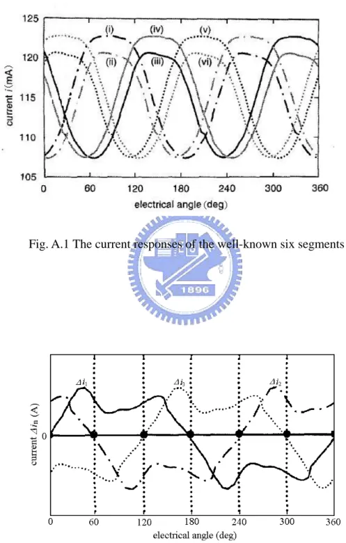
Fig. A.2 The differences between the current in+ and in−...83
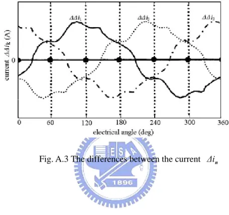
Fig. A.3 The differences between the current∆in ...84
Fig.A.4 The torque generation of the six segments ...86
Index of Tables
Table 2.1 Position based of six segments with Hall-effect sensors signals...14
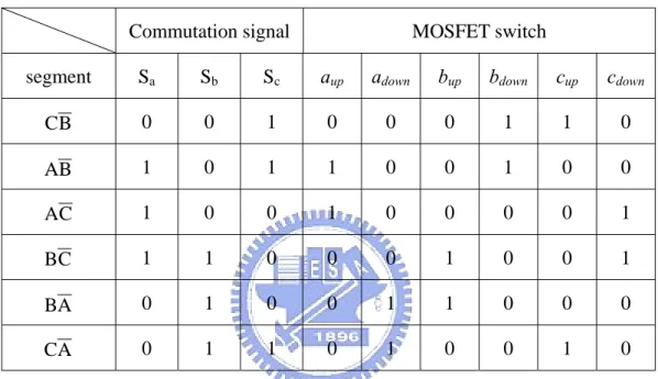
Table 4.1 Six segments of an electrical cycle...38
Table 4.2 Polarity of ddi on rotor position ...40
Table 4.3 The definition of the position sector...43
Table 4.4 The relation between the duty ratio and estimated angular velocity ...43
Table 5.1 The specification of the BLDC motor ...46
Table 5.2 The phase commutation sequence...53
Table A.1 Six segments of an electrical cycle...82
Table A.2 Polarity of ∆∆ik on rotor position ...84
Chapter 1
Introduction
1.1 Background
Nowadays, BLDC motors become more and more attractive for many industrial applications, such as electrical vehicles, compressors and DVD players etc. Comparing with other motors, BLDC motors possess some distinct advantages suchas high torque, high power density and high efficiency. Since BLDC motors use permanent magnet for excitation, rotor position sensors are needed to perform electrical commutation. Conventionally, three Hall-effect sensors are used as rotor position sensors for BLDC motors. However, the sensors lead to several disadvantages, such as cost, size and reliability. In addition, the sensors may be sensitive to the motor temperature inside. Therefore, the sensorless control methods have been widely studied in recent years, such as back-EMF based position estimation method [1]-[3], third harmonic voltage position detection method [5], free-wheeling diode conducting method [6], and Kalman-filter method [4]. The first two methods both use the detected back-EMFs which should be measured at the instant of the unexcited phase. The third method, free-wheeling diode conducting method, uses indirect sensing of the zero-crossing of the back-EMFs to obtain the switching instants of BLDC motors. The Kalman-filter method is a stochastic observer in the least-square sense for estimating the states of
dynamic non-linear systems and it is viable for the on-line determination of the rotor position and velocity of a motor.
Among these control methods, the back-EMF based position estimation method is often used since the back-EMFs could be measured indirectly from the motor’s terminal voltages. When a motor is running, back-EMF is induced in the coil, and the position information of a rotor can be detected by the back-EMF. However, back-EMF is only generated while a motor is running, which requires another initial position detection and start-up algorithm when a motor is at standstill or at low speed with insufficient back-EMF. Many researchers have focused on the open-loop start-up method [6] and inductive sense start-up method [10]-[11]. In this thesis, the detailed realization issues of the sensorless algorithm will be introduced, and be implemented by using a PC-based feedback control system. In addition, the start-up problem will be overcome in the experiment.
1.2 Thesis Organization
The thesis is organized as follows. First, the basic concepts of BLDC motors are introduced in Chapter 2, including the characteristics, mathematical modeling and commutation principle of BLDC motors. Among them, the commutation principle would focus on the conventional electrical commutation with Hall-effect sensors.
In Chapter 3, some snesorless control method will be introduced. First, Kalman-filter based method, third-harmonics voltage position detection method, and free-wheeling diode conducting method will be described. Then the back-EMF based position estimation method used in experiment will be introduced in detail.
Chapter 4 will discuss the start-up strategies, such as open-loop start-up method and inductive sense start-up method. The initial position of the rotor will be detected to avoid the temporary reverse rotation. An additional modified open-loop start-up method will be proposed to solve the start-up problem. Then the start-up procedure used in the implementation will be presented, including initial position detection and start-up from standstill.
Chapter 5 will describe the hardware setup and implementation of sensorless drive. The sensorless control method and start-up method are implemented by the software, Matlab®−Simulink®. This toolbox can help designer establish them easily and directly. Besides, the hardware circuit which is included in the driver circuit and filter circuit is set up by Real-Time workshop® (RTW) of Matlab®. The main idea of the hardware circuit is to realize and verify the sensorless control method. Chapter 6 will show the experimental results to demonstrate the success of BLDC motor drive. Finally, Chapter 7 gives the conclusions.
Chapter 2
Basic Concepts of BLDC Motors
A brushless DC (BLDC) motor is a rotating electric machine where the stator is a classic three-phase stator like that of an induction motor and the rotor has surface-mounted permanent magnets. In this chapter, the basic configuration and the characteristics of BLDC motors will be described in Section 2.1. Then the mathematical modeling will be represented in Section 2.2. Furthermore, a BLDC motor requires an inverter and a position sensor to perform “commutation” because a permanent magnet synchronous motor takes the place of dc motor with brushes and commutators [8]. Thus, the detail commutation and excited procedure will be illustrated in Section 2.3.
2.1 Characteristics of BLDC Motors
In general, a BLDC motor consists of a permanent magnet synchronous motor that converts electrical energy to mechanical energy. The basic configuration of BLDC motors are shown in Fig.2.1. In this figure, it’s clear to see that and the excitation of BLDC motors which consists of permanent magnets is on the rotor and the armature is on the stator. On the other hand, BLDC motors come in 2-phase, 3-phase and 4-phase configuration. Corresponding to its type, the stator has the same numbers of windings.
Out of these, 3-phase motors are the most popular and widely used since 2-phase and 4-phase motors are usually used in small power condition [22]. Furthermore, the hall elements are installed inside the stator to detect the rotor position. Since the 3-phase BLDC motors have three windings which are distributed with 120° in electrical degree apart to each other, the driver structure including the six-step inverters using PWM signals. Thus, the principle of switching is based on electrical angular position information, which is decoded by three Hall-effect sensors.
Permanent magnet rotor Winding
Hall element
2.2 Mathematical Modeling of BLDC Motors
In general, a BLDC motor has a permanent-magnet rotor and its stator windings are wound to generate the trapezoidal back electromotive force (back-EMF), and thus it requires rectangular-shaped stator phase current to produce constant torque. Besides, the two-axis transformation (d, q model) [9], [22], commonly used in PMSM, is not necessary the best choice for modeling and simulating the BLDC motors.
The dynamic equations of BLDC motors with Y-connected stator windings are shown in Fig.2.2. When the neutral point is isolated, the phase currents of BLDC, ias(t), ibs(t), and ics(t), can be expressed as
( )
t +i( )
t +i( )
t =0 ias bs cs (2-1) as i bs i cs iFig.2.2 Equivalent modeling for a BLDC Motor Because the three windings are distributed with
3 2π
in electrical degree apart to each other, the stator current in vector space is generally represented as
( )
( )
( )
( )
3 4 3 2π π j cs j bs as s t i t i t e i t e I = + + (2-2) where ias( )
t ,( )
3 2π j bs t e i , and( )
3 4π j cs t ei are the three phase currents correspondingly. Let λas
( )
θe,t , λbs(
θe,t)
and λcs( )
θe,t be the fluxes related to the three phases of the stator, expressed as( )
( )
( )
( )
j e pm j cs ms j bs ms as s e as t, Li t L i t e L i t e e θ π π λ θ λ = + + 3 + 4 3 2 (2-3)( )
( )
( )
( )
⎟ ⎠ ⎞ ⎜ ⎝ ⎛ − − + + + = 3 2 3 2 3 2π π θ π λ θ λ j e pm j cs ms bs s j as ms e bs t, L i t e Li t L i t e e (2-4)( )
( )
( )
( )
⎟ ⎠ ⎞ ⎜ ⎝ ⎛ − − − + + + = 3 4 3 2 3 4π π θ π λ θ λ j e pm cs s j bs ms j as ms e cs t, L i t e L i t e L i t e (2-5)where Lms and Ls respectively represent the mutual inductance and the self-inductance
of the stator. Besides, λpm is the flux magnitude produced by the permanent magnets, which are assumed sinusoidally distributed in the air-gap.
With a cylindrical stator, the self-inductances of the field windings are independent of the rotor position θ when the harmonic effects of stator slot openings are neglected. Hence, the self-inductance is constant, commonly further decomposed as s L ls ss s L L L = + (2-6)
where takes into account the space-fundamental component of air-gap flux and is corresponding to the field-leakage flux.
ss
L
ls
L
The mutual inductances can be found on the assumption that the mutual inductance is due solely to space-fundamental air-gap flux. Because the phases are
displayed by 3 2π and 2 1 ) 3 2 (± π =−
cos , the mutual inductances are Lms Lss
2 1 −
= (2-7)
The phase-a flux linkage (2-3) can be rewritten as
( ) (
e ss sl) ( )
as ss(
bs( )
cs( )
)
pm e as θ t, L L i t L i t i t λ cosθ λ = + − + + 2 1 (2-8) With balanced three-phase currents, substitution of (2-1) gives(
e)
ss sl as pm e as θ ,t L L i λ cosθ λ ⎟ + ⎠ ⎞ ⎜ ⎝ ⎛ + = 2 3 (2-9) Based on the stator flux in (2-3)-(2-5) and (2-9), the stator voltages, vas(t), vbs(t), and vcs(t), can be formulated as( )
s as( )
as( )
e s as( )
as( )
e pm e as t, Ri t Li t sin dt d t i R t v = + λ θ = + & −ω λ θ (2-10)( )
( )
( )
( )
( )
⎟ ⎠ ⎞ ⎜ ⎝ ⎛ − − + = + = λ θ ω λ θ π 3 2 e pm e bs bs s e bs bs s bs dt t, Ri t Li t sin d t i R t v & (2-11)( )
( )
( )
( )
( )
⎟ ⎠ ⎞ ⎜ ⎝ ⎛ − − + = + = λ θ ω λ θ π 3 4 e pm e cs cs s e cs cs s cs dt t, Ri t Li t sin d t i R t v & (2-12) or in matrix form as ⎥ ⎥ ⎥ ⎥ ⎥ ⎥ ⎥ ⎦ ⎤ ⎢ ⎢ ⎢ ⎢ ⎢ ⎢ ⎢ ⎣ ⎡ ⎟ ⎠ ⎞ ⎜ ⎝ ⎛ − ⎟ ⎠ ⎞ ⎜ ⎝ ⎛ − − + = π θ π θ θ λ ω 3 4 3 2 e e e pm e abc abc s abc sin sin sin L R s s s I I V & (2-13) where L= Lss +Lsl 2 3 , , , and ⎥ ⎥ ⎥ ⎦ ⎤ ⎢ ⎢ ⎢ ⎣ ⎡ = cs bs as v v v abcs V ⎥ ⎥ ⎥ ⎦ ⎤ ⎢ ⎢ ⎢ ⎣ ⎡ = cs bs as abc i i i s I ωe is electrical angular velocity.motor is produced in this moving process. The equation of the instant torque could be shown as
(
)
e co e cs bs as e W , i, i, i T θ θ ∂ ∂ = (2-14)where Wco is the co-energy defined in Fig.2.3, and represented as
∫
∫
∫
+ + = as as bs bs cs cs co di di di W λ λ λ (2-15)Fig.2.3 Characteristic for co-energy
In general, for a p-pole 3-phase motor, the total electrical energy could be shown as
[
]
[
]
( )
⎥ ⎦ ⎤ ⎢ ⎣ ⎡ ⎟ ⎠ ⎞ ⎜ ⎝ ⎛ − + ⎟ ⎠ ⎞ ⎜ ⎝ ⎛ − + + + + + + + = cs e bs e as e pm cs as ms cs bs ms bs as ms cs s bs s as s co i cos i cos i cos p i i L i i L i i L p i L i L i L p W π θ π θ θ λ 3 4 3 2 2 2 2 1 2 2 2 2 (2-16)From (2-14) and (2-16), the electromagnetic torque would be formulated by three phase currents, given as
( )
⎥ ⎦ ⎤ ⎢ ⎣ ⎡ ⎟ ⎠ ⎞ ⎜ ⎝ ⎛ − + ⎟ ⎠ ⎞ ⎜ ⎝ ⎛ − + − = pm e as e bs e cse sin i sin i sin i
p T λ θ θ π θ π 3 4 3 2 2 (2-17)
⎥ ⎥ ⎥ ⎥ ⎥ ⎥ ⎥ ⎦ ⎤ ⎢ ⎢ ⎢ ⎢ ⎢ ⎢ ⎢ ⎣ ⎡ ⎟ ⎠ ⎞ ⎜ ⎝ ⎛ − ⎟ ⎠ ⎞ ⎜ ⎝ ⎛ − − = ⎥ ⎥ ⎥ ⎥ ⎥ ⎥ ⎥ ⎦ ⎤ ⎢ ⎢ ⎢ ⎢ ⎢ ⎢ ⎢ ⎣ ⎡ ⎟ ⎠ ⎞ ⎜ ⎝ ⎛ − ⎟ ⎠ ⎞ ⎜ ⎝ ⎛ − = ⎥ ⎥ ⎥ ⎦ ⎤ ⎢ ⎢ ⎢ ⎣ ⎡ π θ π θ θ λ ω π θ π θ θ 3 4 3 2 3 4 3 2 e e e pm e e e e c b a sin sin sin cos cos cos dt d e e e (2-18)
where ea, eb, and ec are the phase back-EMFs. From (2-17) and (2-18), the relationship
between electromagnetic torque and back-EMFs could be represented as
e cs c bs b as a e i e i e i e p T ω + + = 2 (2-19)
According to the Newton law, the electromechanical equation can be expressed as
(
m e L)
(
e e Jω p T ω B p T − 2 + + = 2 &)
(2-20) which could be rearranged as(
e m e Le Jω B ω T
p
T = 2 & + +
)
(2-21)where J is the motor’s inertia, Bm is the viscous damping, TL is the load torque
2.3 Typical Commutation Principle
The model of the 3-phase Y-connected BLDC motor consists of winding resistances, winding inductances, and back-EMF voltage sources [23]. The typical commutation for a BLDC motor is accomplished by controlling the six inverter switches according to the six-step sequence to produce the phase current waveforms as shown in Fig.2.4. Ideally, the currents are in rectangular shapes, and the stator inductance voltage drop may be neglected [7]. Thus, the sequence of the conducting
phase will be shown in Table 2.1 from Fig.2.4. ea Phase A ia 0 eb Phase B ib 0 ec Phase C ic 0 0° 60° 120° 180° 240° 300° 360° Fig.2.4 Ideal back-EMF and phase current waveform of a BLDC motor
The accurate rotor position sensors are required since the torque production performance largely depends on the relationship between excitation currents and back-EMFs. The rotor position sensing can be achieved by using the Hall-effect sensors for low-cost applications, or by resolving and optical encoders for high-performance applications. In reality, Hall-effect sensors are used most widely for electronic commutation of BLDC motor drives. Fig.2.5 shows the system schematic block diagram of the commutation control for a BLDC motor. This figure is included of the inverter circuit, the equivalent model of a BLDCM, and the feedback the signals of Hall-effect sensor.
The inverter circuit of single-phase is cascaded by two power transistors, such as MOSFETs or IGBTs, as the active elements. Both of them can not conduct at the same time to avoid burning under over-current. Generally, NMOSFETs are selected to be the power transistors for small power motors. Based on the devices characteristics, to turn ON the NMOSFETs, a high gate voltage should be applied [21]. In addition, the six segments are processed in order, which is implemented by the six-step drive.
Generally, the typically commutation is based on the rotor position which is measured by three Hall-effect sensors located in the motor. The Hall-effect signals which would send the position massages are related to the back-EMFs . When the phase back-EMF is through the positive zero-crossing, its Hall signal will become high after 30° delay. On the contrary, when the phase back-EMF is through the negative
Hall-effect sensor Hc Hb Commutation Logic Duty ratio PWM control Ha
zero-crossing, its Hall signal will become low after 30° delay. The timing diagram of back-EMFs and Hall-effect signals are shown in Fig.2.6.
Back-emfs 0 e c eb ea Ha Hb Hc 0° 60° 120° 180° 240° 300° 360° Fig.2.6 The timing diagram of back-EMFs and Hall-effect signals
Since the BLDC motor should be separated in six segments, the three Hall-effect sensors can produce digital signals in three bits as shown in Table 2.1. In the traditional control experiment, it is easy to know the rotor position and velocity because it just decodes the digital signals from Hall-effect sensors and differential the variance of one digital signal.
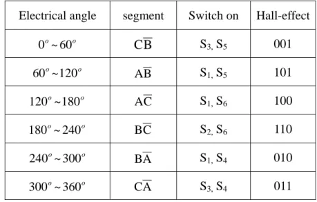
Table 2.1 Position based of six segments with Hall-effect sensors signals Electrical angle segment Switch on Hall-effect
o 0 ~60 o CB S3, S5 001 o 60 ~120o A B S1, S5 101 o 120 ~180o A C S1, S6 100 o 180 ~240o BC S2, S6 110 o 240 ~300o BA S1, S4 010 o 300 ~360o CA S3, S4 011
Ideally, the conducted current waveforms are in rectangular shapes because only two phases are excited at any instant and the effect of free-wheeling diodes is ignored. Hence, the phase current can not be changed suddenly because the inductance exists. In order to analyze the characteristics during the phase commutation, the commutation from phase a-c to phase a-b is considered as an example. First, the diode S1 and S6 in Fig.2.5 will be conducted so that the current of the phase b will pass through the diode. Immediately after switching off Q6, the current of the phase b still pass through the diode until decaying to zero as shown in Fig.2.7. Hence, there exists commutation period between the two-phase conduction period. On the other hand, during the two-phase conducting period, two conducting phase currents are opposite and another one is zero. Therefore, the sum of three phase currents will still equal to zero at any time.
Two-phase conducting period Commutation period Current ia ic Time ib
Chapter 3
Sensorless Commutation Control for BLDC Motors
Since BLDC Motors use permanent magnets for excitation, rotor position sensors are needed to perform electrical commutation. Commonly, three Hall-effect sensors installed inside the BLDC motor are used to detect rotor position. However, the rotor position sensors present several drawbacks from the viewpoint of total system cost, size, and reliability. Therefore, resent investigators have paid more and more attentions to sensorless control without any Hall-effect sensors and proposed many sensorless-related technologies.
Section 3.1 introduces three sensorless control methods. Besides, back-EMF based position detection is more useful than others since the back-EMFs proportional to the rotating angular velocity should be recognized directly or indirectly and the hardware could be realized easily. Hence the back-EMF based position detection will be narrowly described clearly in Section 3.2.
3.1 Review of Sensorless Control Methods for BLDC Motors
Since the knowledge of six communication instants per electrical is only needed for BLDC motors. In order to reduce cost and motor size, the elimination of the rotor position sensors is a very desirable objective in many applications. Furthermore, the sensorless control is the only way for some applications and many methods via sensorless control have been researched, such as back-EMF based position estimation method [1], [2], [3], [19], Kalman-filter based method [4], third-harmonics voltage position detection method [5], and free-wheeling diode conducting method [6]. More details about back-EMF based position estimation method will be discussed in Section 3.2.
3.1.1 Kalman-filter based method
A method which uses the extended Kalman filter (EKF) to estimate speed and rotor position of a BLDC motor is illustrated in [4]. The estimation algorithm is based on the state-space model of the motor and a statistical description of the uncertainties which is modeled by covariance matrices, including P(t), Q(t), and R(t). Define that P(t) is for the system state vector, Q(t) is for the model uncertainty, and R(t) is for the measurement uncertainty.
the prediction and correlation equations, the drive system could be described as
( )
t f[
x( ) ( )
t ,u t ,t]
n( )
tx& = + (3-1)
where the initial state vector is modeled as a Gaussian random vector with mean and covariance , while is a zero-mean white Gaussian noise independent of and with a covariance matrix
( )
t0x
0
x P0 n
( )
t( )
t0x Q
( )
t . The measurement are modeled as( )
ti h[
x( )
ti t,i]
v( )
tiy = + (3-2)
where is a zero-mean white Gaussian noise independent of and with a covariance matrix . Hence, the EKF would generate a minimum-variance estimator since it has a predictor-corrector structure.
( )
tiv x
( )
t0( )
tiR
However, there exists a critical part since the design is to use accurate initial value for the various covariance matrices. In principle, these initial matrices need to be obtained by considering the stochastic properties of the corresponding noises. Since these noises are usually unknown, trial-and-error method is used for tuning the initial estimates of these matrices to obtain the best tradeoff between filter stability and convergence time.
3.1.2 Third-harmonics voltage based detection method
This method in [5] deals with the use of the third harmonic component of the back-EMF for indirect sensing the rotor flux position. The six step inverters switch the
stator excitation at every π3 electrical degree. The switching can be detected by
monitoring the third-harmonic voltage of the back-EMF. The stator voltage equation for phase a, for instance, is written as
( )
as as s as s as i e dt d L i R v = + + (3-3)Similar expressions can be written for the other two stator phases. The phase stator resistance and inductance are represented as Rs and Ls respectively. The term eas
represents the back-EMF voltage. For a full pitch magnet and full pitch stator phase winding, the back-EMF voltages contains the following frequency components
(
cosωt k cos3ωt k cos5ωt k cos7ωt ...)
E eas = e + 3 e + 5 e + 7 e + (3-4)
(
)
(
)
(
cos ωt / k cos3 ωt / ...)
E ebs = e −2π 3 + 3 e −2π 3 + (3-5)(
)
(
)
(
cos ωt / k cos3ωt / ...)
E ecs = e +2π 3 + 3 e +2π 3 + (3-6) Because of Y-connected stator windings, the third-harmonic voltage component atthe terminal voltage is only due to the back-EMF. The summation of the three stator phase voltages is a zero sequence which contains a dominant third-harmonic component and high frequency components, expressed as
high_freq 3 high_freq e 3 cn bn an v v 3Ek cos3ωt v v v v + + = + = + (3-7)
where v3 is the third-harmonic voltage and vhigh_freq is the high frequency components.
Therefore, the rotor flux can be estimated from this third-harmonic signal by integrating the resultant voltage v3,
(3-8)
∫
= v dt λr3 3
Since the third harmonic flux linkage lags the third harmonic of the back-EMF voltages by 30 degrees, the commutation signals can be obtained by directly detecting the zero-crossing of the third harmonic flux linkage without any phase delay. Fig.3.1 shows the relationship between the back-EMFs, the third harmonic voltage and the rotor flux linkage; it is clearly to see that the zero-crossing of is the commutation instant. The result of the summation of the three phase voltages contain the third-harmonic voltage and high frequency sequence components that can be easily eliminated by a low-pass filter.
3
r λ
To sum up, the important advantages of this method are easy to implementation
v3
0
0° 60° 120° 180° 240° 300° 360° Fig.3.1 Relationship between the back-EMFs, the third harmonic voltage and
the rotor flux linkage
ea eb ec 0 3 λ 0
and low susceptibility to electrical noise. On the other hand, signal detection at low speeds with this method is possible because the third harmonic signal has a frequency three times higher than the fundamental back-EMF, allowing operation in a wider speed range than techniques based on sensing the motor back-EMF. However, it is difficult to sense the neutral point voltage. Therefore, the neutral terminal is not available due to the cost and structure constrains in application.
3.1.3 Free-Wheeling diode conducting method
Since the back-EMF is quite small and hard to detect during the low-speed operation, it is difficult to precisely detect the rotor position based on the back-EMF only. Recently, some approaches have included other information besides back-EMF to detect the rotor position, for example the work by S. Ogasawara and H. Akagi [6]. Their approach proposed a method on the basis of the conducting state of free-wheeling diodes connected with power transistors. Fig.3.2 shows the circuit with phase a-b conducted, which means the active signal is given to S1 and S5. If S1 is on state, the dc link voltage increases the main current i. If S1 turn off, the current i continues to flow through the free-wheeling diode D4 and decreases. Then, the voltage equation of this loop can be derived as
0 = + + + − + + + S S a b S S CE F V dt di L i R e e i R dt di L V (3-9)
where VCE and VF denote the forward voltage drop of the transistors and diode. From
(3-9), the voltage drop of the motor winding as 2 2 F CE b a S S V V e e dt di L i R + =− − − − (3-10)
The neutral voltage vn which also shown in Fig.3.2, is given by
a S F b S CE n e dt di L i R V e dt di L i R V v = + + − =− − − − (3-11)
Substitution (3-10) into (3-11) gives the following equation 2 2 b a F CE n e e V V v = − − + (3-12)
Since the c-phase terminal voltage vc equals ec+ , vvn c is given as
2 2 b a F CE c n c c e e V V e v e v = + = + − − + (3-13)
Equation (3-13) holds good even in transient states because no motor constant are included. The conducting condition of the diode D6 is given by
F
c V
v <− (3-14)
Substituting (3-13) into (3-14) gives the following equation 2 2 F CE b a c V V e e e − + <− + (3-15)
Since the back-EMF are assumed in ideal trapezoidal waveform, is approximately zero near the zero point of . Therefore, the conducting condition of D6 is given by b a e e + c e 2 F CE c V V e <− + (3-16)
In general, VCE and VF are much smaller than the back-EMF. When the back-EMF ec become negative, the open-phase current flows through the negative-sign diode D6.
Therefore, the zero-crossing point of the non-excited phase back-EMF can be equivalently obtained by detecting corresponding diode conducting condition. Fig.3.3(a) shows a current waveform in an open phase, and Fig.3.3(b) shows a specially designed circuit to detect whether the free-wheeling diodes are conducting or not. A resistor and a diode are connected to a comparator for voltage clamping. The reference voltage is slightly smaller than the forward voltage drop of the free-wheeling diode. After detecting the diode conducting instant in the non-excited phase, a digital phase shifter is realized to generate the correct commutation signal. However, the detecting circuit needs two isolated power supplies and the external hardware circuit is required.
ref
V VF
Fig.3.2 Free-wheeling conducting circuit in active signal S1 to S5
i Vdc
VCE
Fig.3.3 Free-wheeling diode conducting method: (a) current waveform in an open phase, (b) Diode conducting detecting circuit
3.2 Back-EMF Based Position Estimation Method
The rotor position is obtained directly by measurement of the back-EMFs induced in the stator windings. In the basic operation of a BLDC motor, only two phases are energized at any instant with the other phase unexcited. Therefore, each of the motor terminal voltages contains the back-EMF information that can be used to derive the commutation instants [1], [19]. The zero-crossing method is employed to determine the switching sequence by detecting the instant where the back-EMF in the unexcited phase crosses zero. After detecting the commutation instant, the phase shifter is needed to get the correct commutation signal.
3.2.1 Zero-crossing detection
Generally, with Y-connected stator windings, the terminal voltages va, vb and vc can be
derived as n a a a n an a e v dt di L Ri v v v = + = + + + (3-17) n b b b n bn b e v dt di L Ri v v v = + = + + + (3-18) n c c c n cn c e v dt di L Ri v v v = + = + + + (3-19)
where vn is the neural voltage, van, vbn and vcn are the phase voltages, ia, ib and ic
represent the phase currents, and ea, eb and ec are the phase back-EMFs generated in
the three unexcited phase. From (3-17) to (3-19) can be derived as
(
an bn cn)
nc b
a v v v v v v
v + + = + + +3 (3-20) Note that the current of the non-excited phase is zero if all the winding currents applied to the three phases are assumed to possess ideal rectangular shape without any disturbance. Hence, from (3-17) to (3-20), the back-EMF of the non-excited phase a can be derived as
(
)
[
a b c a]
a n a a v v v v v v e e = − = − + + − 3 1 (3-21) By simplifying (3-21), ea can be estimated as follows
(
)
⎥⎦ ⎤ ⎢⎣ ⎡ − + + = a a b c a v v v v e 3 1 2 3 (3-22) From (3-21) and (3-22), when ea reaches to zero point, va can be estimated as(
a b c)
n a v v v v v = + + = 3 1 (3-23)The relationship between three terminal voltages and the waveform of back-EMF produced from (3-22) are shown in Fig.3.4. Therefore, the positions of the zero-crossing point could be detected from the back-EMF of phase a ( ) when the electrical angles in the region of 0°-60° and 180°-240° as shown in Fig.3.4. In additional,
and could be found in the same way.
a e non b e − ec−non Vdc v a
After comparing the signals as presented in Fig.3.5, It could be found the relationship between the non-excited phase back-EMF ( ) and Hall-effect signals (Ha). Thus, the zero-crossing points of the non-excited phases are required to be
a e
(
)
⎥⎦⎤ ⎢⎣ ⎡ − + + = a a b c a v v v v e 3 1 2 3 dc V 4 3 − Vdc/2(
a b c)
n v v v v = + + 3 1 Vdc Vdc vc vb 0 0 0 V 4 3 dc V 4 3 0° 60° 120° 180° 240° 300° 360° Fig.3.4 Ideal three terminal voltages and the waveform of back-EMFdelayed with 30 electrical degrees for generating the corresponding commutation signals instead of Hall-effect signals. The System schematic of sensorless BLDC motor drive is presented in Fig.3.6. Compared with System schematic of typical commutation control in Fig.2.5, the zero-crossing detection has replaced three Hall-effect sensors.
Zero-crossing signal Ha a e 0° 60° 120° 180° 240° 300° 360° Fig.3.5 The relationship between the non-excited phase back-EMF
The method can be realized by using voltage sensors and low pass filters. However, the modulation noise is eliminated by using the low pass filters which is produced a phase delay varies with the frequency of the excited signal for the desired speed. Besides, since the back-EMF is zero at standstill and proportional to rotor speed, this method can not be used at zero speed and realizes difficultly at startup or very low situation.
3.2.2 Commutation phase shifter
After recognizing the zero-crossing signal of the estimated non-excited phase back-EMF, an additional 30° phase shift is required to perform correct commutation. Since the precision of the sensorless commutation control depends on the rotor speed, a
a b c n Phase Voltage Zero-crossing detection Commutation Logic PWM control Duty ratio
novel frequency-independent phase shifter (FIPS) [3] has been proposed. The algorithm of this phase shifter has been proven independent of input signal frequencies. However, the computation effort is quite large for real-time application; hence the digital simplified-type FIPS has been proposed in [1] as shown in Fig.3.7. Define the variable γ as the ratio of decreasing to increasing increments for the counters, cp
( )
kand , which are limited by a positive value L to avoid overflow condition at very low speed. Thus, and
( )
k cn( )
k cp cn( )
k can be expressed as( )
(
( )
)
(
( )
)
⎪⎭ ⎪ ⎬ ⎫ ⎪⎩ ⎪ ⎨ ⎧ ⎥ ⎥ ⎦ ⎤ ⎢ ⎢ ⎣ ⎡ ⎟ ⎠ ⎞ ⎜ ⎝ ⎛ + − − =∑
= L , m x sgn m x sgn max min k c k k m p p γ 2 1 2 1 0, (3-24)( )
(
( )
)
(
( )
)
⎪⎭ ⎪ ⎬ ⎫ ⎪⎩ ⎪ ⎨ ⎧ ⎥ ⎦ ⎤ ⎢ ⎣ ⎡ ⎟ ⎠ ⎞ ⎜ ⎝ ⎛ + − − =∑
= L , m x sgn m x sgn max min k c k k m n n γ 2 1 2 1 0, (3-25) with( )
⎪⎩ ⎪ ⎨ ⎧ < − ≥ = 0 if 1 0 if 1 x , x , x sgn (3-26)where kp is the largest k as cp
( )
k −cp(
k−1)
<0, and is the largest k as . Fig.3.8 illustrates the operational waveform of the proposed phase shifter. Assume that the input signaln
k
( )
k −c(
k−1)
<0cn n
( )
kx in Fig.3.7 is the zero-crossing signal of the non-excited phase back-EMF as shown in Fig.3.5, and the output is the corresponding commutation signal. Also, since commutations exist every 180° in Fig.3.5,
( )
ky
*
φ π
γ = (3-27)
where is the desired degrees of the phase shift. Therefore, the decreasing increments are six-times larger than the increasing increments in order to make the phase shift = 30°. Besides, k
*
φ
*
φ zn denotes the time when nth zero-crossing of input
signal x
( )
k occurs, and kcn denotes the time when the commutation occurs. Bydefinition, kp is the largest k when cp
( )
k −cp(
k−1)
<0, hence kp=kc1 when k=kc1. As aresult, the output signal y
( )
k is changed from +1 to −1 at kc1 and the counter of cp( )
kis disabled until next zero-crossing is triggered. On the other hand, is the largest k when
n
k
( )
k −c(
k−1)
<0cn n , hence kn=kc2 when k=kc2. As a result, the output signal
is changed from −1 to +1 at k
( )
ky c2 and the counter of cn
( )
k is disabled until nextzero-crossing is triggered. Therefore, the proposed digital phase shifter not only
performs the frequency-independent characteristics, but also reduces computation effort.
P x ( )k cn N x ( )k cp
kp= kc1 kp= kc1 kp=0 kn= kc2 kn=0 kn=0 0 0 1 -1
( )
k x k 0 k k k( )
k y( )
k cn( )
k cp kz1 kc1 kz2 kc2 kz3 kc3Chapter 4
Start-up Strategy and Procedure for BLDC Motors
The start-up strategy is necessary since there is little or no back-EMF to sense when the motor is standstill or at a low speed. This chapter will introduce the start-up strategy in detail and the implementation of initial position detection and the start-up procedure for the BLDC motors.
4.1 Start-up Strategy
Since the back-EMF detection based position detection method cannot be used at start-up or low-speed, the additional start-up strategies are needed to solve these problems. Generally, the open-loop start-up algorithm can avoid this problem, in which strong current is flown to the output driver to force the rotor to move to the known rotor position [1], [20]. This open-loop algorithm has disadvantages of slow start and possibility of initial backward rotation [6]. Instead of open-loop start-up, inductive sense start-up algorithm is widely used in BLDC motor applications nowadays [10], [21]. In this section, these two methods will be introduced in detail.
4.1.1 Open-loop start-up method
The open-loop start-up method is accomplished by providing a rotating stator field which increases gradually in frequency. Once the rotor field begins to become
attracted to the stator field enough to overcome friction and inertia, the rotor begins to turn. However, the drawback of this method is the initial rotor movement is not predictable, which is inadequate for disk drives. Thus, the initial position detection is important in this method.
The motor starting procedure will be illustrated as follows: first, the rotor would be aligned from an unknown position to a certain position. Then set control signals to the driver circuit with a conducting sequence. If the initial position could be known accurately, this method could succeed in high probability.
4.1.2 Inductive sense start-up method
The main idea of this method is to utilize the fact that the inductance of the motor winding varies as the rotor position changes. The magnetic flux generated by the current in the stator winding can increase or decrease the flux density in the stator depending on the rotor position, leading to decrease or increase in induction due to the saturation of the stator. The relationship between inductance and flux linkage is shown as Li + = PM Phase λ λ (4-1)
where λPhase is the summation of the flux from the permanent magnet, λ , and the PM flux from the current i. L is the inductance of the excited phase. Supply the current with positive or negative direction to the phase, as shown in Fig.4.1 [10]. The
variations of the inductance are derived as + + + + = − = i ∆λ i λ λ L Phase PM (4-2) − − − − = − = i ∆λ i λ λ L Phase PM (4-3)
where and are the inductance and flux linkage variation corresponding to the positive current is provided; , and is opposite. It is obvious that is smaller than due to is smaller than . Consider the response of a phase voltage and current to the variation of the inductance. The phase voltage equation is expressed as + L ∆λ+ + i L− ∆λ− i− + L L− ∆λ+ ∆λ− a an e dt di L Ri v = + + (4-4)
The back-EMF can be neglect when a motor is at standstill. Then, solve the differential equation; the phase current can be derived as
⎟⎟ ⎠ ⎞ ⎜⎜ ⎝ ⎛ − = − tL R e R v i an 1 (4-5)
According to (4-5), the phase current has a different transient dependent on the inductance variation, which is determined by the relative position of the magnet and the direction of the current. It should be noted that has a faster response than due to the time constant is larger than , as shown in Fig.4.2 [10]. Therefore, the position information can be obtained by monitoring the phase current
and in an appropriate time interval.
+ i i− + R/L R/L− + i i−
− ∆λ + ∆λ λPM i i+ i− λphase
Fig.4.1 The flux linkage with positive or negative current
∆i R van i | i− | i+ T t
Fig.4.2 The responses of current with positive or negative direction
By applying positive and negative voltage pulses sequentially and measuring the difference in inductance, it can be determined which magnetic polarity the phase
winding is facing (Appendix A). Therefore, the initial position can be detected by the difference of the current pulse.
After identifying the initial position when a motor is at standstill, the correct phases winding on the stator are excited and the maximum electromagnetic torque is produced so that motor starts to rotate. Necessarily, the next commutation position should be detected for next excitation when the rotor rotates with 60 electrical degrees. However, the method proposed in previous section is not suitable while the rotor is rotating due to the time delay caused by the period of six voltage pulses and the negative direction torque produced by exciting incorrect segments. The start-up procedure proposed by G. H. Jang, J. H. Park and J. H. Chang [10] will be detailed illustrated in Appendix A.
However, the success of this algorithm strongly depends on how sensitive the inductance of the phase winding to the direction of the applied current at the given position. Therefore, the prototype motor which was unsuccessful with the inductive sense start-up algorithm will be investigated using finite element method (FEM) analysis for the identification of the root cause [13].
4.2 Start-up Procedure
In the section will verify the method introduced in Section 4.1 and represent the start-up procedure which will be used in the experiment for the BLDC motor since the start-up procedure is highly dependent on the characteristics of the motor.
4.2.1 Initial position detection
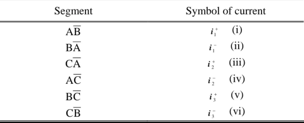
By using the initial position detection mentioned in Section 4.1, the relation of each segments of an electrical cycle will be implemented. As shown in Table 4.1, the three-phase motor has six segments of an electrical cycle, in which any two phases out of three currents. In order to verify the feasibility of this method, measured the current response with a delay 500µs. Besides, by using (4-5), the inductance is determined whenever a rotor moves the electrical angle of 12°. Therefore, Fig.4.3 could be plotted to show the relative rotor position with respect to the stator produces different response of the current i1+ and i1-. In addition, Fig.4.4 shows the variation of the difference
responses , which can provide information on the rotor position because the polarity of changes every electrical angle of 60°, where di
di di 1= 1 1 , di − + − i i 2= and di − + − 2 2 i i
3=i3+ − i3− . The equilibrium positions (P1~P6), which means the relative magnitudes
Table 4.1 Six segments of an electrical cycle
Segment Symbol of current B A i1+ A B i1− A C i2+ C A i2− C B i3+ B C i3− 0 60 120 180 240 300 360 2.6 2.8 3 3.2 3.4 3.6 3.8 4 4.2 4.4 4.6
electrical angle (deg)
cu rr en t ( A m p ) i1+ i 1
0 60 120 180 240 300 360 -0.8 -0.6 -0.4 -0.2 0 0.2 0.4 0.6 0.8
electrical angle (deg)
cur re n t di ( A m p ) di 1 di2 di3 P1 P2 P3 P4 P5 P6
Fig.4.4 First difference of current responses to the rotor position
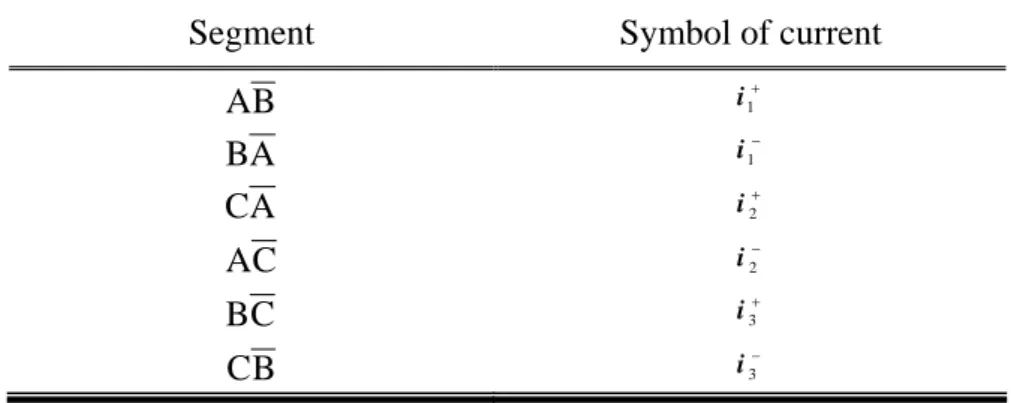
However, it is very difficult to identify the polarity of di near the magnetic equilibrium where a rotor tends to stop, because one of three di is zero in these positions. In these case, the polarity of second different of the current response, ddi, can be effectively used to identify the rotor position. Fig.4.5 shows the for electrical period, where ddi
ddi
1= di1-di2, ddi2= di2-di3, and ddi3= di3-di1. Therefore, the
polarity of ddi provides information on the rotor position near the equilibrium positions as shown in Table 4.2. Consequently, the stationary rotor position can be detected by ministering the polarity of di and ddi to energize the correct phases of the motor.
0 60 120 180 240 300 360 -1 -0.8 -0.6 -0.4 -0.2 0 0.2 0.4 0.6 0.8 1
electrical angle (deg)
c u rr ent ddi ( A m p ) ddi 1 ddi 2 ddi3 P 1 P2 P3 P4 P5 P6
Fig.4.5 Second difference of current responses to the rotor position
Table 4.2 Polarity of ddi on rotor position
Electrical position ddi1 ddi2 dd i3 0ο ~ 60ο − + − 60ο ~ 120ο + + − 120ο ~ 180ο + − − 180ο ~ 240ο + − + 240ο ~ 300ο − − + 300ο ~ 360ο − + +
4.2.2 Start-up from standstill
Consider the sampling rate is not high enough to implement the start-up algorithm proposed in [10] (see Appendix A.2), the open-loop method is used form standstill to the low angular velocity. After using the initial position detection to ensure the starting point, the next position should be right to avoid the initial backward rotation. However, the conventional open-loop method could not make the motor rotating smoothly from standstill since the torque input from software is too high. Therefore, the modified open-loop start-up method is proposed by using voltage pulse as shown in Fig.4.6.
Define the six segments as sector 0~5 which are shown in Table 4.3. After detecting the initial sector, a set of position sequence will import the system and the motor will start to rotate in right direction. However, time delay is caused since the command instant is always faster than the motor arriving instant. Fig.4.7 shows the relation between the command signal and the circuit signal with initial sector 0. At
t t tc 2tc 3tc 4tc B A AC BC BA B A AC v v 0 0 tc 2tc
starting, the delay time is almost beyond a commutation time. After a period of time, the delay time will become less and approach to a constant. Then the system will switch to the commutation algorithm because there are enough back-EMFs to be detected.
As mentioned before, if there is no initial position detection, the initial backward will be incurred. For example, when the rotor initial position is in the sector 3 but the command is started in the sector 1, the rotor will rotate backward at the first commutation period as shown in Fig.4.8.
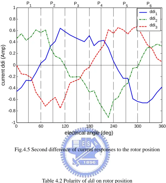
In addition, the angular velocity could be estimated by the commutation period because six commutation periods are equal to an electrical cycle. The mathematical equation is shown as 2 6 60 p t ˆ c× × = ω (4-6)
where p is pole number and tc is the commutation period. Since the velocity is changed
by tuning the duty ratio, Table 4.4 will show the relation between the duty ratio and estimated angular velocity of the motor. By using the table, the open-loop start up method can be used from standstill to accelerate the velocity with decreasing time interval in the command signal.
Table 4.3 The definition of the position sector Segment Electrical position Sector
B C 0 ~o 60 o 0 B A 60 ~o 120o 1 C A 120 ~o 180o 2 C B 180 ~o 240o 3 A B 240 ~o 300o 4 A C 300 ~o 360o 5
Table 4.4 The relation between the duty ratio and estimated angular velocity Duty ratio (%) Angular velocity (rpm) tc (ms) 2 12.8997 9.6901 10 13.0691 9.5645 20 49.0097 3.5105 30 76.0586 1.6435 40 100.1600 1.2480 50 117.1875 1.0667 60 130.7909 0.9557 70 140.1903 0.8916 80 148.6549 0.8409 90 155.6351 0.8032 100 170.4790 0.7332
0 1 2 3 4 5 6 7 8 9 10 0 1 2 3 4 5 time Se c to r command signal circuit signal
Fig.4.7 The relation between the command signal and the circuit signal
0 1 2 3 4 5 6 7 8 9 10 0 1 2 3 4 5 time Se c to r command signal circuit signal
Chapter 5
Hardware Setup and Implementation of Sensorless
Drivers
The theories and sensorless control strategies for the BLDC motor have been introduced in Chapter 3 and 4. In order to fulfill the control strategies, it is required to design sensorless drivers with good performance. Hence, this chapter will focus on the implementation of sensorless drivers. Besides, some experiments using PC-based drive system will be set up to verify the developed sensorless control strategies.
5.1 Experimental System Descriptions
The whole experimental system shown in Fig.5.1 consists of a BLDC motor, a driver circuit, AD/DA card, a PC-based control unit and a set of low-pass filters. The motor divers will be discussed in Section 5.2.
BLDC Motor Driver Circuit xPC Control unit Sensorless control algorithm & PWM AD/DA card PCI-6024E Filter Velocity transducer Fig.5.1 The complete hardware PC-based control system
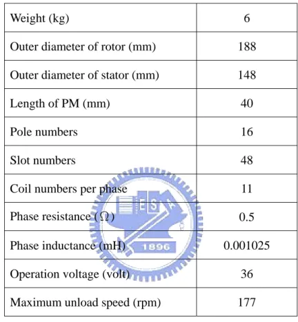
A 3-phase BLDC axial-flux wheel motor, Crystalyte 4011, is used as the experimental plant, which is a low speed and high torque direct-drive motor with specifications listed in Table 5.1.
Table 5.1 The specification of the BLDC motor
Weight (kg) 6
Outer diameter of rotor (mm) 188 Outer diameter of stator (mm) 148
Length of PM (mm) 40
Pole numbers 16
Slot numbers 48
Coil numbers per phase 11 Phase resistance (Ω) 0.5 Phase inductance (mH) 0.001025 Operation voltage (volt) 36 Maximum unload speed (rpm) 177
In the second part, the AD/DA card, which is named PCI-6024E, is an I/O broad with 16 single analog input (A/D) channels, 2 analog output (D/A) channels, 8 digital input and output lines. The maximum input sampling rate is 200kHz and the output sampling rate is 10kHz.
On the other hand, the control unit and AD/DA card are connected by the xPC target environment [12] which is shown in Fig.5.2, using two PC connected by
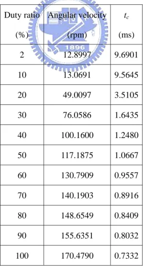
![Fig 5.4 The functional block diagram of IR2113 [14]](https://thumb-ap.123doks.com/thumbv2/9libinfo/8620138.191442/63.892.171.732.523.799/fig-functional-block-diagram-ir.webp)