國立交通大學
電機學院 IC 設計產業研發碩士班
碩 士 論 文
整合於
H.264/AVC HDTV 解碼器的無失真嵌入式壓縮方法
A Lossless Embedded Compression Codec Engine
Integrated with H.264/AVC HDTV Decoder
學生 : 洪建州
指導教授 : 李鎮宜 教授
整合於
H.264/AVC HDTV 解碼器的無失真嵌入式壓縮方法
A Lossless Embedded Compression Codec Engine
Integrated with H.264/AVC HDTV Decoder
研 究 生:洪建州 Student:Chien-Chou Hung
指導教授:李鎮宜 Advisor:Dr. Chen-Yi Lee
國 立 交 通 大 學
電機學院 IC 設計產業研發碩士班
碩 士 論 文
A Thesis
Submitted to College of Electrical and Computer Engineering National Chiao Tung University
in Partial Fulfillment of the Requirements for the Degree of
Master in
Industrial Technology R & D Master Program on IC Design
January 2008
Hsinchu, Taiwan, Republic of China
整合於
H.264/AVC HDTV 解碼器的無失真嵌入式壓縮方法
學生:洪建州 指導教授:李鎮宜 教授
國立交通大學
電機學院產業研發碩士班
摘要
在本論文中,我們提出一個有效的無失真嵌入式壓縮器,在無損畫面品質的要求下來減 少對系統頻寬的存取。 所提出的演算法能夠利用畫面預測的結果來選擇三種掃描模式,以提高 DPCM 的壓縮效 能,經過 DPCM 所產生的預測錯誤將會被更進一步地利用 Golomb-Rice 編碼方法來壓縮;為 了避免被壓縮的檔案無限制的擴展,每一個被壓縮的分割檔案必須小於 128 位元大小的限 制。如果碼長預測器發現分割檔案違反了我們的限制,它將會直接傳送原來的像素值到系統 匯流排而不壓縮它。根據實驗的結果,所提出的演算法能夠實現超過 2 的平均壓縮率而且畫 面品質不會被犧牲。 所提出的硬體架構能夠工作在每秒 30 張畫面的 HDTV 系統裡而工作頻率為 120MHz。 利用 UMC 0.18um 的製程技術,所提出的硬體架構只需要 22.5K 的邏輯閘數目而功率消耗為 3.3mW。與所減少的系統頻寬存取相比較,所消耗的面積與功率是相當的小。A Lossless Embedded Compression Codec Engine
Integrated with H.264/AVC HDTV Decoder
Student: Chien-Chou Hung Advisor: Dr. Chen-Yi Lee
Industrial Technology R & D Master Program of
Electrical and Computer Engineering College
National Chiao Tung University
ABSTRACT
In this thesis, we propose an efficient lossless embedded compression codec engine to reduce the system bus access without quality degradation.
The proposed algorithm can make use of the intra prediction results to choose the three scan modes that could enhance compression efficiency of DPCM. The prediction errors after DPCM will furthermore be compressed by Golomb-Rice coding. In order to prevent infinite expansion of the compressed bitstream, the compressed segment must be less than 128 bits limitation. If the code length predictor finds that the compressed segment violates our constraint, it will transfer original pixels to the system bus. According to the experiment results, the proposed algorithm can achieves the average of compression ratio more than 2 and no quality will be sacrificed.
The proposed architecture can decode at HDTV@30fps with 120MHz clock rate. Based on UMC 0.18 um CMOS technology, the proposed architecture needs 22.5K gate counts and power consumption is 3.3mW. Compared with the amount of the reduced system bus access, the area and power overhead is small.
誌
謝
工作一段時間後,沒想到有機會可以重拾往日學生生活,雖然開心,但更多一些近鄉情 怯的感覺。但是隨著研究逐漸地完成,從中所學到的東西與獲得的經驗,讓我更有自信,在 此由衷的感謝曾經幫助我、關心我的人。 首先要感謝的是 李鎮宜 教授。在面對研究上的困境時,能夠在老師的指導下不斷的往 前推進,學習真正的研究方法與知識,讓我在面對問題時,能夠從系統的架構來分析問題的 原因。另外,我也要感謝我的口試委員:蔣迪豪教授、張添烜教授和黃俊達教授,非常感謝 您在百忙之中抽空參與我的口試,並且提供許多寶貴的建議,讓我獲益良多。 接著要感謝的是 mingle 和李曜的大力協助。因為有你們的體諒及幫忙,不厭其煩的指出 我研究中的缺失,且總能在我不知所措時為我解惑,讓研究能夠更完整而嚴謹。另外,實驗 室的韋磬、阿德、昱帆、超人,你們的幫忙及搞笑我銘感在心。 兩年裡的日子,實驗室裡共同的生活點滴,學術上的討論、圖書館外的閒扯、趕作業的 革命情感、因為遲到而遮遮掩掩閃進實驗室會議…,感謝所有 SI2 研究室的學長、同學、學 弟妹的共同砥礪,你們的陪伴讓兩年的研究生活變得多彩多姿。 最後,我要感謝我的爸爸媽媽,因為有您的支持才能順利完成學業。以及我的老婆俸如, 謝謝妳陪伴在我的身邊。
Contents
CHAPTER 1 INTRODUCTION ...1
1.1 OVERVIEW OF H.264/AVCVIDEO STANDARD... 1
1.2 MOTIVATION... 2
1.3 THESIS ORGANIZATION... 3
CHAPTER 2 REVIEWS OF PRIOR WORKS...5
2.1 LOSSY EMBEDDED COMPRESSION ALGORITHM... 5
2.2 LOSSLESS EMBEDDED COMPRESSION ALGORITHM... 6
2.3 MULTI-MODE EMBEDDED COMPRESSION ALGORITHM... 6
2.4 SUMMARY... 7
CHAPTER 3 LOSSLESS EMBEDDED COMPRESSION ALGORITHM INTEGRATED WITH H.264/AVC DECODER...8
3.1 CHARACTERIZE THE FUNCTIONALITIES OF PROPOSED ALGORITHM... 9
3.1.1 Scan Modes Decision ... 9
3.1.2 Pixel-wise DPCM ... 13
3.1.3 Golomb-Rice Coding and Segment Packing... 17
3.1.4 Code Length Prediction ... 19
3.2 AN EXAMPLE OF THE PROPOSED ALGORITHM... 21
3.3 SIMULATION RESULTS... 23
CHAPTER 4 HARDWARE ARCHITECTURE DESIGN INTEGRATED WITH H.264/AVC
HDTV DECODER ...26
4.1 MEMORY CONTROLLER... 27
4.2 MEMORY CONTROLLER INTERFACE AND SDRAMORGANIZATION... 28
4.3 THE SYSTEM ARCHITECTURE FOR LOSSLESS EMBEDDED COMPRESSION ALGORITHM31 4.3.1 The Architecture of Pixel-wise DPCM with Four Scan Modes ... 33
4.3.2 The Architecture of Code Length Predictor ... 35
4.3.3 The Architecture of Golomb-Rice Coding with Packing ... 37
4.4 THE SYSTEM ARCHITECTURE FOR LOSSLESS EMBEDDED DECOMPRESSION ALGORITHM... 39
4.4.1 The Architecture of Synchronous FIFO with Barrel Shifter ... 40
4.4.2 The Architecture of Golomb-Rice Decoder ... 42
4.4.3 The Architecture of Inverse Scan Modes ... 43
4.5 SUMMARY... 44
CHAPTER 5 EXPERIMENTAL RESULTS ...46
5.1 PERFORMANCE EVALUATION... 46
5.2 IMPLEMENTATION RESULTS... 47
5.3 COMPARISON WITH RELATED WORKS... 49
5.4 SUMMARY... 50
CHAPTER 6 CONCLUSION AND FUTURE WORK ...51
6.1 CONCLUSION... 51
6.2 FUTURE WORK... 51
List of Figures
FIG.1.THE PRESENTED SCHEME INTEGRATED WITH H.264/AVCHDTV DECODER... 3
FIG.2.THE FLOWCHART OF THE PROPOSED LOSSLESS EMBEDDED COMPRESSION ALGORITHM... 9
FIG.3.NINE PREDICTION MODES FOR THE INTRA 4 X 4 PREDICTION IN THE H.264 STANDARD... 10
FIG.4.EIGHT KINDS OF SCAN MODES... 11
FIG.5.THE FLOWCHART OF THE CONVENTIONAL DPCM FOR SPATIAL PREDICTION... 13
FIG.6.THE FLOWCHART OF THE PROPOSED PIXEL-WISE DPCM... 14
FIG.7.AN EXAMPLE OF PIXEL-WISE DPCM ALONG SCAN MODE 1... 14
FIG.8.THE ALLOCATION OF FIRST PIXELS AND NEIGHBORING PIXELS IN A MACROBLOCK... 16
FIG.9.(A)A COMPRESSED SEGMENT FORMAT AND (B)AN UNCOMPRESSED SEGMENT FORMAT... 19
FIG.10.AN EXAMPLE OF 4X4 BLOCK WITH SCAN MODE 1... 22
FIG.11.THE SAVING BIT RATE ON VARIOUS TEST SEQUENCES... 25
FIG.12.THE BLOCK DIAGRAM OF THE SI2LAB’S H.264/AVCHDTV DECODER WITH LOSSLESS EMBEDDED COMPRESSION CODEC ENGINE... 27
FIG.13.THE BLOCK DIAGRAM OF THE MEMORY CONTROLLER WITH LOSSLESS EC CODEC ENGINE... 28
FIG.14.THE BLOCK DIAGRAM OF SDRAM ORGANIZATION... 29
FIG.15.THE 4X4 REFERENCE PIXEL VALUES AMONG FOUR COMPRESSED SEGMENTS... 30
FIG.16.SUB-PIXEL MOTION COMPENSATION... 30
FIG.17.THE 9X9 REFERENCE PIXEL VALUES AMONG NINE COMPRESSED SEGMENTS... 30
FIG.18.A VIRTUAL TO PHYSICAL ADDRESS MAPPING... 31
FIG.20.THE PROPOSED PIPELINING SCHEME FOR ENCODER SCHEDULING... 33
FIG.21.THE ARCHITECTURE OF PIXEL-WISE DPCM WITH FOUR SCAN MODES... 34
FIG.22.THE ARCHITECTURE OF CODE LENGTH PREDICTOR... 36
FIG.23.THE ARCHITECTURE OF GOLOMB-RICE CODING WITH PACKING... 38
FIG.24.THE LOSSLESS EMBEDDED COMPRESSION DECODER... 39
FIG.25.THE ARCHITECTURE OF SYNCHRONOUS FIFO WITH BARREL SHIFTER... 41
FIG.26.THE ARCHITECTURE OF GOLOMB-RICE DECODER... 42
FIG.27.THE ARCHITECTURE OF INVERSE SCAN MODES... 43
List of Tables
TABLE1:MEMORY ACCESS RATIO OF EACH H.264/AVC DECODER MODULE... 2
TABLE2: THE PROBABILITY OF THE SHORTEST CODE LENGTH FOR EACH INTRA PREDICTION MODE12 TABLE3: SCAN MODE DECISION... 12
TABLE4: AN EXAMPLE OF GOLOMB-RICE CODEWORD WITH K =3 ... 20
TABLE5: THE FIXED CODE LENGTH OF PARAMETERS FOR EACH 4X4 BLOCK... 21
TABLE6: THE COMPRESSED SEGMENT OF THE BLOCK THAT SHOWN IN FIG.10 ... 22
TABLE7: THE COMPRESSION RATIO WITH DIFFERENT QP VALUES... 24
TABLE8: DESIGN CONCEPTION OF PACKING... 37
TABLE9: DESIGN CONCEPTION OF GOLOMB-RICE DECODING... 40
TABLE10: THE IMPLEMENTATION RESULTS OF THE PROPOSED LOSSLESS EMBEDDED COMPRESSION CODEC ENGINE... 44
TABLE11: THE REQUIRED OPERATION FREQUENCY IN DIFFERENT VIDEO FORMATS IN OUR PROPOSED DESIGN... 45
TABLE12: THE AVERAGE COMPRESSION RATIO WITH DIFFERENT QP VALUES ON VARIOUS TEST SEQUENCES... 47
Chapter 1
Introduction
1.1 Overview of H.264/AVC Video Standard
The H.264/AVC is the new generation video coding standard jointly developed as ITU-T Recommendation H.264 and ISO/IEC 14496-10 (MPEG-4 Part 10) Advanced Video Coding (AVC) [1]-[2]. It supports several powerful coding tools to improve coding efficiency, such as flexible block size motion estimation, quarter pixel motion compensation, multiple reference frames, spatial intra prediction, in-loop de-blocking filters and context-based adaptive binary arithmetic coding, etc. It provides efficient lossy coding of video content and saves the bit rate by approximately 30%–70% when compared with previous video coding standards such as MPEG-4 Part 2 [3], H.263 [4], H.262/MPEG-2 Part 2 [5], etc. Nevertheless it preserves the same or better image quality.
To address the requirement for the most-demanding professional environments, the JVT (Joint Video Team: ITU-T Video Coding Experts Group and ISO/IEC Moving Picture Experts Group) recently completed the new amendment and some extensions to the original standard that are known as the Fidelity Range Extensions (FRExt) [6]. These extensions [7] enable higher quality video coding by supporting increased sample bit depth precision and higher-resolution color information, including sampling structures known as YUV 4:2:2 and YUV 4:4:4. Several other features are also included in the Fidelity Range Extensions project, such as adaptive switching between 4×4 and 8×8 integer transforms, encoder-specified perceptual-based quantization weighting matrices, efficient inter-picture lossless coding, and support of additional color spaces.
Therefore, the H.264/AVC FRExt has been adopted as an industrial standard by consortiums for digital high-definition television (HDTV) broadcasting and storage applications like HD-DVD
and Blu-ray disc.
1.2 Motivation
The H.264/AVC could achieve much higher coding efficiency than those previous standards; however, it also increases complexity both in a large amount of computation and ultra high memory bandwidth in the hardware implementation of H.264/AVC HDTV decoder. For platform-based video systems in which the high computation requirement can be easily solved by increasing the parallelism of processing elements, the real challenge is the unacceptable bus bandwidth requirement with limited system resources.
There are four main modules require external memory access in H.264/AVC HDTV decoder [8], which are reference picture store, de-blocking, display feeder and motion compensation. In addition, there some other external memory access requirements such as stream store and motion vector store, as they are much less than the four main modules, they are ignored from consideration. TABLE 1 lists the memory access ratio of each module in H.264/AVC HDTV decoder in the worst case. We can see that motion compensation module is the main memory access bottleneck of H.264/AVC HDTV decoder. Therefore, minimization of memory access operations is a key consideration in H.264/AVC HDTV decoder hardware design.
TABLE 1: Memory access ratio of each H.264/AVC decoder module (W: frame width, H: frame height)
Module name Max memory access bytes Ratio(≈)
Ref. picture store W*H + 2*(W/2)*(H/2) 10%
De-blocking (W/16)*(H/16-1)*16*4*2*2 5%
Display feeder W*H + 2*(W/2)*(H/2) 10%
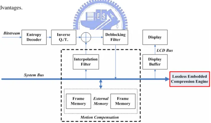
A block-based embedded compression will compress block-based video data generated by video coding system before transferring to system bus. It would be monitored by a bus controller before connecting to memory. Hence embedded compression codec engine could reduce the bandwidth requirement because the amount of fetched data is compressed. FIG. 1 shows the presented scheme is integrated with H.264/AVC HDTV decoder to reduce the external memory access when loading motion compensation and reduce system bus access when displaying.
For the purposed scheme, many algorithms and implementations of embedded compression for various video coding system are presented [9]–[21] in recent years. Existing embedded compression algorithms can be divided into two groups: lossy embedded compression algorithms and lossless embedded compression algorithms. In the following section, we will further discuss on lossy and lossless embedded compression codec engines about their own advantages and disadvantages.
FIG. 1. The presented scheme integrated with H.264/AVC HDTV decoder
1.3 Thesis Organization
Chapter 2. The lossless embedded compression algorithm integrated with H.264/AVC decoder is proposed in Chapter 3. Furthermore, the architecture of the proposed algorithm integrated with H.264/AVC HDTV decoder is proposed in Chapter 4. Some performance evaluation and implementation results are shown in Chapter 5, moreover, comparison with related works is shown in this chapter. Finally, the contributions of this thesis and other issues that are worth to have further discussion and research are made in Chapter 6.
Chapter 2
Reviews of Prior Works
In this section, some literatures are discussed and they are divided into third parts. The first is to review the existing lossy embedded compression algorithm. The second is to introduce existing lossless embedded compression algorithm. Finally, the multi-mode embedded compression algorithm is introduced in the third part.
2.1 Lossy Embedded Compression Algorithm
A popular technique for lossy embedded compression algorithm is a transform-based approach in which a frame is decomposed into small blocks that are transformed into a frequency domain by a simple transform such as DCT, Hadamard Transform or its variations [16]. Then, the frequency domain coefficients are compressed by quantization followed by variable length encoding such as Golomb-Rice coding. This approach, in general, requires a large amount of computation to reduce the quality degradation by compression algorithm. Another approach is a downsampling-based compression algorithm [17] that requires a relatively small amount of computation, but the quality may be degraded due to the loss of an edge pattern in the course of downsampling for compression and upsampling for decompression. Another spatial domain compression based on DPCM is proposed in [18] and an adaptive vector quantization scheme is presented in [19].
Lossy embedded compression with fixed compression ratio [10]-[20] can guarantee the size of compressed data of each block. Thus it is able to reduce not only external memory access but also the requirement of external memory size. However lossy embedded compression is not suitable for any kind of applications if the high video quality requirement is necessary. It will lead to quality degradation due to the error propagation (i.e. drift effect). Therefore it is more suitable for video
conferencing or video on mobile hand-held systems where quality is of much less important or Scalable Video Coding (SVC) systems with motion-compensated temporal filtering scheme.
2.2 Lossless Embedded Compression Algorithm
Lossless embedded compression [9] can guarantee no quality loss of video data, and hence no drifting effect exists in the video systems. But it will produce uncertain compressed size of each block. Therefore lossless embedded compression can not reduce the memory size, but it can still reduce the access power of external memory and bandwidth requirement of the system bus.
2.3 Multi-Mode Embedded Compression Algorithm
A recent researcher proposed a multi-mode compression method by adopting a Set-Partitioning in Hierarchical Trees (SPIHT) algorithm [21] to support both lossy and lossless compression. Because the SPIHT algorithm features to simply reach lossy/lossless compression, fixed compression ratio, rate and quality control, hence it has been adopted for a purposed of frame re-compression.
Although the SPIHT algorithm has many good properties that make it suitable for embedded compression codec engine, there are two main disadvantages for SPIHT in VLSI design. The first disadvantage of SPIHT algorithm is the large buffer size between DWT and SPIHT. DWT is a word-level arithmetic process, while the SPIHT engine encodes/decodes coefficients bitplane by bitplane. Moreover, being different with EBCOT in JPEG 2000, SPIHT requires image-level access. This means that when coding one bitplane, the entire current bitplane must be available. This mismatch of the data flow between DWT and SPIHT coding engine makes it necessary to buffer DWT coefficients of entire image. This also makes the latency between the first input and the first output to be at least the duration of performing DWT of entire image.
straightforward implementation of SPIHT, 6L2 × log2L (L is the image width) bits are needed for
the LIS, LIP, and LSP buffers in SPIHT algorithm. This buffer size is even larger than the image itself. The buffer inside SPIHT engine with size more than a quarter of image size is needed, and this is also too large for a low-cost design.
Therefore, although researcher presented an efficient architecture, it still cannot reach high-definition real-time compression and decompression duo to the extensive processing cycles.
2.4 Summary
From the discussion above, we review the existing methods and classify a great diversity of existing algorithms as well. We could find that those algorithms are stand-alone methods. That means most of previous methods are performed independently of a video compression standard and therefore do not take advantage of the information obtained during the processing of the compression standard.
For the real-time H.264/AVC HDTV video decoder, the high video quality requirement is necessary; hence we will desire no quality degradation due to the embedded compression. Therefore lossless embedded compression codec engine is adopted for our proposed method integrated with H.264/AVC HDTV decoder. And we might make use of helpful information from H.264/AVC to achieve high compression efficiency, low complexity and high throughput architecture for reducing bandwidth requirement of the system bus.
Chapter 3
Lossless Embedded Compression
Algorithm Integrated with H.264/AVC
Decoder
To achieve the requirements of our proposed method integrated with H.264/AVC decoder, the proposed lossless embedded compression algorithm is presented in this chapter. All those aforementioned methods are performed independently of the video coding standard and therefore do not take advantage of the information obtained during the processing of the coding standard. The recent researcher proposes a new compression algorithm that makes use of the information from H.264 intra prediction results [20]. Our proposed method is bases on this idea and moreover improves the compression efficiency to be suitable for our lossless compression requirement.
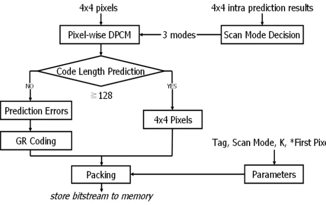
The flowchart of the proposed algorithm is shown in FIG. 2. In the H.264/AVC decoder, intra prediction result is the best mode among 9 possible prediction modes for every 4x4 blocks. Since the selected mode gives information about the characteristic of the 4x4 block, the proposed algorithm uses this information to select the three kinds of scan modes for the 4x4 block and performs DPCM along this scan order. The code length predictor could select the shortest code length among three kinds of the scan modes and further compressed by Golomb-Rice coding. If the code length predictor calculates the total code length of the 4x4 block exceed 128 bits limit, we will directly transfer the 4x4 pixels to the system bus. As a result, the proposed algorithm achieves the average compression ratio of more than 2 without quality degradation.
FIG. 2. The flowchart of the proposed lossless embedded compression algorithm
3.1 Characterize the Functionalities of Proposed Algorithm
In this section, we would discuss the functionality of each block diagram as shown in FIG. 2. They are characterized as follows:3.1.1 Scan Modes Decision
For the compression efficiency of DPCM, the prediction errors between successive data must be small so that the data can be represented by a small number of bits. The amount of the prediction errors depend on the image type of a 4x4 block as well as the scan order. For example, if a certain 4x4 block has vertical stripes, a scan order along the vertical direction is more efficient than that along the horizontal direction. Therefore, it is important to select the scan direction that is suitable for a given image data.
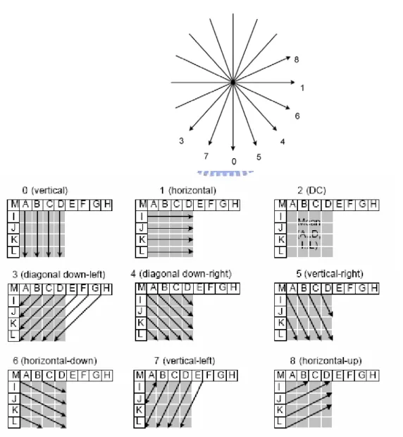
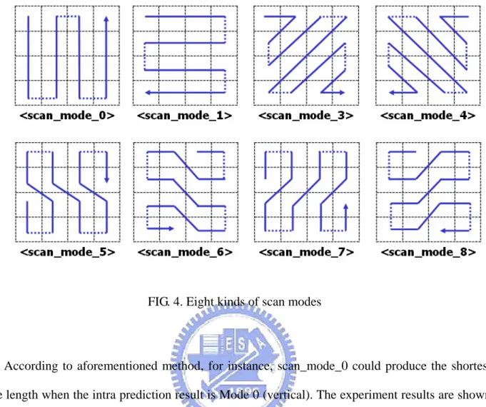
chosen, with conceptual prediction directions as illustrated in FIG. 3 (mode 2, not shown in the figure, is the “DC” averaging mode). The recent researcher [20] presented eight different scan modes as shown in FIG. 4 in which the arrowed lines show the scan order. These eight modes are similar to the intra 4x4 prediction modes. Note that H.264/AVC 4x4 intra prediction has nine different modes and scan_node_2 (the DC mode) is in excluded in FIG. 4 because the DC mode does not give much information for a scan order selection. The eight modes cover various image types for DPCM scan. For example, scan_mode_0 is suitable for an image with vertical stripes while scan_mode_1 is suitable for horizontal stripes. An image with diagonal stripes may be suitable for one of the other modes.
FIG. 4. Eight kinds of scan modes
According to aforementioned method, for instance, scan_mode_0 could produce the shortest code length when the intra prediction result is Mode 0 (vertical). The experiment results are shown in TABLE 2. This table represents that when the intra prediction is given to the 4x4 block, each of scan modes is able to produce the probability of the shortest code length. Both scan_mode_0 and scan_mode_1, in general, produce efficient compression results, especially when intra prediction modes are Mode 5, Mode 6, Mode 7 and Mode 8; Moreover, the contribution of scan_mode_5, scan_mode_6, scan_mode_7 and scan_mode_8 to lossless compression algorithm achieves little.
Therefore in order to reduce hardware complexity and power consumption, moreover, enhance compression efficiency; the 4x4 intra prediction result is given to the algorithm to decide three scan modes among the four modes as shown in TABLE 3. Both scan_mode_0 and scan_mode_1 are always selected as the first and second modes. If intra prediction results are Modes 1, 2, 3, 7, and 8, then scan_mode_3 is selected as the third mode, or else the other intra prediction results are Modes 0, 4, 5, and 6, then scan_mode_4 is selected as the third mode. Such constitution is able to ensure
the probability of the shortest code length by more than 70%.
TABLE 2:
The probability of the shortest code length for each intra prediction mode Unit: (%)
scan 0 scan 1 scan 3 scan 4 scan 5 scan 6 scan 7 scan 8
Mode 0 65.41 7.42 4.73 5.58 7.24 2.44 5.22 1.96 Mode 1 17.09 51.48 6.69 5.18 4.41 6.45 2.92 5.78 Mode 2 36.17 18.04 12.46 9.03 8.13 5.44 6.10 4.63 Mode 3 25.97 18.15 30.94 4.39 4.71 3.03 6.57 6.24 Mode 4 32.65 13.28 4.32 28.40 10.58 5.91 2.82 2.05 Mode 5 54.68 4.85 2.23 19.79 13.66 2.07 1.75 0.98 Mode 6 18.48 35.73 5.06 19.22 5.95 9.43 2.43 3.70 Mode 7 46.86 9.35 19.84 3.09 4.82 2.14 10.59 3.30 Mode 8 25.46 30.01 18.74 3.90 4.36 4.08 5.34 8.11 TABLE 3: Scan mode decision
Intra Prediction Result 0 1 2 3 4 5 6 7 8
3.1.2 Pixel-wise DPCM
A simple and well-known method for spatial prediction is to predict the present pixel value based on the pervious values and further encode prediction errors by entropy coder. This method is called DPCM. In general, best predictors are those form the neighboring pixels. In order to achieve coding efficiency for lossless compression, the selected scan orders are given to the next step that performs third DPCM operations along the selected scan orders.
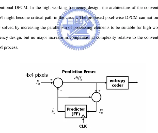
The flowchart of the conventional DPCM is shown in FIG. 5. It has a disadvantage in hardware implementation as each prediction error taking one clock cycle is necessary; hence we propose a pixel-by-pixel (pixel-wise) DPCM that is more flexible in hardware design as illustrated in FIG. 6. The prediction errors of the proposed pixel-wise DPCM are still the same as of the conventional DPCM. In the high working frequency design, the architecture of the conventional DPCM might become critical path in the circuit. The proposed pixel-wise DPCM can not only be easily solved by increasing the parallelism of processing elements to be suitable for high working frequency design, but no major increase in computational complexity relative to the conventional DPCM process.
FIG. 6. The flowchart of the proposed pixel-wise DPCM
FIG. 7. An example of pixel-wise DPCM along scan mode 1
The following is an example of the pixel-wise DPCM. Consider a 4x4 block given as shown in FIG. 7. Assume that the scan mode is 1. The first_pixel and the prediction errors diff1, diff2... and
diff15 of each pixel P0, P1... and P15 are calculated by pixel-wise DPCM as follows:
13 12 15 2 3 3 1 2 2 0 1 1 0 _ P P diff P P diff P P diff P P diff P pixel first − = − = − = − = =
The pixel-wise DPCM always requires each individual decoded pixel to be provided sequentially prior to the prediction and reconstruction of the next pixel value. As an example, in order to reconstruct pixel P3, pixel P2 should be reconstructed, in other words, pixel P0 and pixel
P1 have been already reconstructed. Therefore we can reconstruct the 4x4 block from the
prediction errors when scan mode is 1 as follows:
0 15 2 1 12 0 3 2 1 3 0 2 1 2 0 1 1 _ 0 P diff diff diff P P diff diff diff P P diff diff P P diff P pixel first P + + + + = + + + = + + = + = = …
And it also could be expressed in matrix form to provide the high throughput architecture in hardware design as follows:
⎥
⎥
⎥
⎥
⎥
⎥
⎥
⎥
⎥
⎥
⎥
⎦
⎤
⎢
⎢
⎢
⎢
⎢
⎢
⎢
⎢
⎢
⎢
⎢
⎣
⎡
⎥
⎥
⎥
⎥
⎥
⎥
⎥
⎥
⎥
⎥
⎥
⎦
⎤
⎢
⎢
⎢
⎢
⎢
⎢
⎢
⎢
⎢
⎢
⎢
⎣
⎡
=
⎥
⎥
⎥
⎥
⎥
⎥
⎥
⎥
⎥
⎥
⎥
⎦
⎤
⎢
⎢
⎢
⎢
⎢
⎢
⎢
⎢
⎢
⎢
⎢
⎣
⎡
15
5
4
3
2
1
_
1
1
1
1
1
1
1
1
0
0
1
1
1
1
1
1
0
0
1
1
1
1
1
0
0
0
1
1
1
1
0
0
0
0
1
1
1
0
0
0
0
0
1
1
0
0
0
0
0
0
1
12
6
7
3
2
1
0
diff
diff
diff
diff
diff
diff
pixel
first
P
P
P
P
P
P
P
…
The first_pixel is the entry pixel of a 4x4 block along the scan order. Suppose that the scan mode is 1, it is the P0 as shown in FIG. 7. The first_pixel should be compressed to achieve coding efficiency for lossless compression. In our proposed lossless compression algorithm, pixel-wise DPCM would involve neighboring pixel that is close to the first pixel and produce predicted error between first pixel and neighboring pixel as shown in FIG. 8.
FIG. 8. The allocation of first pixels and neighboring pixels in a macroblock
The H.264/AVC has a block-based coding structure. In its design, each picture is segmented into macroblocks, which consist of an array of 16x16 luma samples and two associated two arrays of 4x4 chroma samples. Each sample is further decomposed into several 4x4 blocks. In the H.264/AVC decoder, the block 0 that containing 16 pixels is reconstructed first for a macroblock. Next, the other blocks 1-23 are reconstructed in the order as illustrated in FIG. 8.
In order to simplify hardware design, the first pixels and the neighboring pixels are located in the fixed position. Therefore, the first_pixel is placed on the up-left corner of a 4x4 block and the neighboring pixel that is chosen very close to the first pixel as shown in FIG. 8. According to experiment results, the pixel-wise DPCM involving neighboring pixel could significantly enhance compression efficiency by approximately 0.1 of compression ratio, but no major increase in hardware complexity and power consumption.
3.1.3 Golomb-Rice Coding and Segment Packing
Before talking about code length prediction in section 3.1.4, we should discuss Golomb-Rice coding first [22]-[23]. Although an arithmetic coding is the best-known lossless coding method, it requires expensive iterative coding and decoding procedures and consumes large computing power. On the other hand, the DPCM output, prediction errors, diffn are in [-255, 255]. If they are
compressed by Huffman coding, Huffman code may result in a long codeword and computationally-intensive coding and decoding. Therefore we adopt Golomb-Rice coding to translate the prediction error into a codeword for the low-complexity design.
Golomb codes of parameter m encode a positive integer value by encoding value mod m in binary followed by an encoding of value div m in unary. When m = 2k the encoding procedure has a very simple realization and has been referred to as Rice coding in the literature, hence following we refer to them as Golomb-Rice codes. The Golomb-Rice coding accepts only a non-negative number as its input when a DPCM result can be a negative number. Therefore, a DPCM result is converted into a non-negative number as follows:
(1)
.
,
1
2
,
0
,
2
otherwise
for
diff
diff
for
diff
value
−
=
≥
=
(2) Where diff represents a DPCM result and value represents the input to the Golomb-Rice coding. The conversion back from value to diff is simple because the LSB of value indicates whether diff is a negative or not. The mapping value orders prediction residuals, interleaving negative values and positive values in the sequence 0, -1, 1, -2, 2, … If the values follow a Laplace distribution centered at zero, then the distribution of value will be close to (but not exactly) geometric, which can then be encoded using an appropriate Golomb-Rice code.The key factor behind the effective use of Golomb-Rice codes is the estimation of the coding parameter k to be used for a given sample or block of samples. If k is smaller, the code length increase is too large for a large value. On the other hand, if k is greater, the code length is too large
for a small value. Weinberger's algorithm [24] exhaustively tries codes with each parameter on a block of samples and selects the one which results in the shortest code length. The coding parameter k is computed as follows:
(3)
}
2
|
min{
k
kN
valueA
valuek
=
′
′⋅
≥
The k is estimated by maintaining in each context value, the count Nvalue of the number of times the
context value has been encountered so far and Avalue, the accumulated sum of magnitudes of
prediction errors within this context value. This strategy is an approximation to optimal parameter selection for Golomb-Rice coding.
Based on aforementioned formulation applied in our proposed algorithm, Nvalue and Avalue
could be written as follows:
∑
==
=
15 016
n n value valuevalue
A
N
(4) (5) The coding parameter k could be computed as follows:(6)
}
4
log
|
min{
}
16
2
|
min{
2−
≥
′
′
=
≥
⋅
′
=
′ value value kA
k
k
A
k
k
(7) Therefore, it also could be expressed in the following priority conditions in hardware implementation:If the coding parameter k is more than six, the total code length after Golomb-Rice coding will exceed 128 bits limitation. Therefore k equal to six is the upper bound of the code length limitation.
10 9 9 8 8 7 7 6 6 5 5 4 4
2
2
,
6
,
2
2
,
5
,
2
2
,
4
,
2
2
,
3
,
2
2
,
2
,
2
2
,
1
,
2
0
,
0
≤
<
=
≤
<
=
≤
<
=
≤
<
=
≤
<
=
≤
<
=
≤
≤
=
value value value value value value valueA
k
A
k
A
k
A
k
A
k
A
k
A
k
After precise estimation of the coding parameter k, the total number of bits generated by Golomb-Rice coding for all prediction errors can be reduced.
The parameters and Golomb-Rice codes or 16 pixels of a block are packed as a small than or equal to 128-bit segment respectively. FIG. 9 (a) shows a compressed segment format and (b) an uncompressed segment format. In order to differentiate between compressed and uncompressed segments, we use one bit as a judgment (tag) and stored in the leftmost position, the four scan modes are coded with 2 bits and the 3-bit k is stored next. The first pixel requires 8 bits stored next to the k and the remaining bits store the 15 Golomb-Rice codes for the remaining pixels.
tag (1 bits) scan_mode (2 bits) k (3 bits) *first_pixel (8 bits) prediction errors after Golomb-Rice coding
(a) Total less than 128 bits
tag
(1 bits)
16 pixels of a block
(b) Total 128 bits
FIG. 9. (a) A compressed segment format and (b) An uncompressed segment format
3.1.4 Code Length Prediction
In the section 3.1.3, we explicitly discuss the algorithm of Golomb-Rice coding. An example of Golomb-Rice codeword with k = 3 is shown in TABLE 4. Each value divided by 2k produces a quotient and a remainder. Then Q indicated quotient is transformed into unary code and R indicated remainder is transform into fixed-length code.
TABLE 4:
An example of Golomb-Rice codeword with k = 3
value Q R codeword value Q R codeword
0 0 0 1000 8 1 0 01000 1 0 1 1001 9 1 1 01001 2 0 2 1010 10 1 2 01010 3 0 3 1011 11 1 3 01011 4 0 4 1100 12 1 4 01100 5 0 5 1101 13 1 5 01101 6 0 6 1110 14 1 6 01110 7 0 7 1111 15 1 7 01111
Hence we could find Golomb-Rice code is variable length code with a regular construction. It is constructed in a logical way:
[Prefix][1][Suffix]
Prefix has Q-bit leading zeros and Suffix has a k-bit remainder value. Therefore the code length of a Golomb-Rice code and of all prediction errors as follows:
k Golomb
value
k
Length
2
1
+
+
=
(8))
2
1
(
15 0 _ k n n errors predictionvalue
k
Length
=
∑
+
+
= (9)The parameters for each 4x4 block are shown in TABLE 5. The fixed code length of all parameters is: (10)
13
=
parametersLength
TABLE 5:
The fixed code length of parameters for each 4x4 block
Parameters Type No. of bits
scan_mode scan_mode_0 scan_mode_1 scan_mode_3 scan_mode_4 2 k 0~6 3 first_pixel unsigned 8
The pixel-wise DPCM would produce 3 kinds of prediction errors for given 3 scan modes. Code length prediction could decide the shortest code length among prediction errors and further compressed by Golomb-Rice coding. If total code length of a 4x4 block exceeds 128 bits limitation, we will directly transfer the 4x4 pixels to the system bus. According to (9) and (10), the total code length limitation condition could be formulated as follows:
(11)
128
_
≥
+
=
parameters prediction errorstotal
Length
Length
Length
3.2 An Example of The Proposed Algorithm
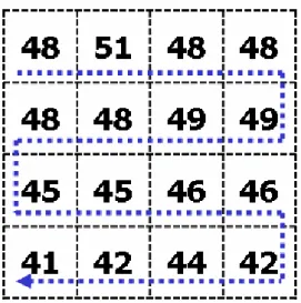
Consider a 4x4 block given as shown in FIG. 10. Assume that the scan mode is 1. The compression result is given in TABLE 6 which tag equal to 1 is indicated that the total code length is less than 128 bits. 1 is chosen for the k-value. Note that k-value more than 6 requires 134 bits which are not acceptable. The scanned data in the order of scan mode 1 is 48, 51, 48, 48, 49, 49, 48, 48, 45, 45, 46, 46, 42, 44, 42 and 41.
FIG. 10. An example of 4x4 block with scan mode 1
TABLE 6:
The compressed segment of the block that shown in FIG. 10
Element value Rice-mapping Code
tag 1 N/A 1 scan_mode 1 N/A 01 k 1 N/A 001 *first_pixel 48 N/A 00110000 diff[1] 3 6 00010 diff[2] -3 5 0011 diff[3] 0 6 10 diff[4] 1 2 010 diff[5] 0 0 10 diff[6] -1 1 11 diff[7] 0 0 10 diff[8] 3 6 0011
diff[9] 0 0 10 diff[10] 1 2 010 diff[11] 0 0 10 diff[12] -4 7 00011 diff[13] 2 4 0010 diff[14] -2 3 011 diff[15] -1 1 11
Total code length 59
3.3 Simulation Results
The software implementation of the proposed algorithm is integrated with JM8.2 reference software of the H.264/AVC main profile and the reconstructed frame from de-blocking filter is compressed by the proposed algorithm. The lossless embedded compression algorithm is evaluated with 18 test video sequences with CIF (352 x 288) resolution. For all test sequences, 100 frames are used with QP = 5, 10 and 15 respectively. FIG. 11 shows the saving bit rate with QP = 5 and furthermore the compression ratio with different QP values on various test sequences as shown in TABLE 7.
TABLE 7:
The compression ratio with different QP values
Seq. Proposed CR Seq. Proposed CR Seq. Proposed CR
QP 5 1.9354 QP 5 1.9516 QP 5 2.0942 QP 10 1.9643 QP 10 1.9725 QP 10 2.1614 trevor QP 15 2.0090 hall_ monito r QP 15 2.0331 carphone QP 15 2.2508 QP 5 2.4516 QP 5 1.6125 QP 5 1.8728 QP 10 2.6020 QP 10 1.6184 QP 10 1.9126 miss_am QP 15 2.7728 mobile QP 15 1.6291 foreman QP 15 1.9712 QP 5 2.1826 QP 5 1.9986 QP 5 1.7905 QP 10 2.2463 QP 10 2.0546 QP 10 1.8096 suzie QP 15 2.3300 news QP 15 2.1244 salesman QP 15 1.8626 QP 5 2.0397 QP 5 1.8114 QP 5 2.6210 QP 10 2.1223 QP 10 1.8387 QP 10 2.7789 akiyo QP 15 2.3196 silen t QP 15 1.8774 claire QP 15 2.8622 QP 5 1.8252 QP 5 1.7107 QP 5 2.0381 QP 10 1.8728 QP 10 1.7280 QP 10 2.1062 coastguard QP 15 1.9026 stefan QP 15 1.7478 grandma QP 15 2.2102 QP 5 1.9707 QP 5 1.7959 QP 5 2.0285 QP 10 2.0234 QP 10 1.8181 QP 10 2.0941 container QP 15 2.0873 table QP 15 1.8951 mother_dau. QP 15 2.1884
FIG. 11. The saving bit rate on various test sequences 0 10 20 30 40 50 60 70 1 7 13 19 25 31 37 43 49 55 61 67 73 79 85 91 97 Frame Number sav in g bi ts ( % ) mo_daughter grandmother claire salesman foreman carphone akiyo container coastguard hall_monitor news silent table suzie miss_am trevor
3.4 Summary
According to the experiment results mentioned above, we could find the compression efficiency depending on the picture complexity in each frame. The distribution of saving bit rate in each frame is normally average and the proposed lossless embedded compression algorithm achieves the average of compression ratio more than 2 without quality degradation.
Chapter 4
Hardware Architecture Design Integrated
with H.264/AVC HDTV Decoder
A lossless embedded compression codec engine is integrated with the SI2 Lab’s H.264/AVC HDTV decoder and it is embedded in the memory controller as shown in FIG. 12. The reconstructed frame is generated by de-blocking filter and sent to the memory controller with lossless embedded compression codec engine that compresses and stores the data in the frame memory. For decompression, the data is read from the frame memory through memory controller, decompressed and then sent to inter prediction unit for motion compensation.
In this chapter, proposed memory controller for lossless embedded compression codec engine is presented in section 4.1. Memory controller interface and SDRAM organization is presented in section 4.2. The implementation of lossless embedded compression and decompression algorithms are presented in section 4.3 and 4.4 respectively. Finally, summary is described in section 4.5.
FIG. 12. The block diagram of the SI2 Lab’s H.264/AVC HDTV decoder with lossless embedded compression codec engine
4.1 Memory Controller
FIG. 13 shows the block diagram of the memory controller with lossless embedded compression codec engine we propose. The memory controller is placed between system bus and many clients, i.e. IP blocks. The system bus transfers data after each other for many clients. The carrying data consists of stream buffering, motion vectors buffering, reference picture store, de-blocking, display feeder and motion compensation, etc. When image data passes over the bus, a controller activates the lossless embedded compression codec engine. The compression unit reduces the amount of data to be transferred; hence, the transfer length is reduced.
The system bus is shared among many clients. Although our proposed scheme is lossless compression, in other words, any kind of data could be compressed as well as the compressed data could be converse back original data. But proposed compression algorithm is developed for image data. We can not guarantee the compression performance for the other non-image data. Hence the
controller must not only recognize whether data is image type but also decide whether data will be compressed. If system bus traffic is executed in transactions, the image data needs to be compressed. Otherwise, the image data are forwarded uncompressed. Although image data could be compressed by compression unit, however we still need to take a system architect's perspective including bus arbitration, bus scheduling and the memory access protocols in order to achieve higher system bus utility.
FIG. 13. The block diagram of the memory controller with lossless EC codec engine
4.2 Memory Controller Interface and SDRAM Organization
After receiving bitstream from the memory controller, we apply a data packing to send the packed results into a data word-line on SDRAM. FIG. 14 depicts the SDRAM organization and each word-length is of size 32-bit. And the memory address from the deblocking filter uses directmapping method. As an example, assume compression ratio is 2. For a write operation, the compression unit receives the start address A and 16 bytes of image data. The data will be compressed to 8 bytes of data, which is stored at the address A. The remainder 8 bytes of address space is not used. At a read transaction on address A, the signal processing unit requests 16 bytes of image data. Only 8 bytes of data are actually read from the memory. The compression unit decompresses this to 16 bytes of image data, which is passed to the requesting bus client. The address scheme our proposed is uncomplicated but wastes many memory space. Maybe we can achieve higher memory utility through address mapping, can be made for the further research.
FIG. 14. The block diagram of SDRAM organization
Because the motion compensation module requires the reference pixel values in SDRAM, a compressed pixel is difficult for data addressing from SDRAM. As an example, assume a integer-pixel compensation, the motion compensation requires the 4x4 reference pixel values among four compressed segments that are stored in the SDRAM as shown in FIG. 15. We must decode the four compressed segments first and then transfer 4x4 reference pixel values to the motion compensation. Consider the worst case, sub-pixel compensation, the motion compensation
requires 1/2 and 1/4 pixel compensation as shown in FIG. 16. The motion compensation requires the 9x9 reference pixel values among nine compressed segments as shown in FIG. 17. Hence motion compensation can not accept the extra latency duo to the decoding many compressed segments that are stored in the SDRAM. In order to solve this problem, we may increase the parallelism of processing elements to achieve motion compensation requirements.
FIG. 15. The 4x4 reference pixel values among four compressed segments
FIG. 16. Sub-pixel motion compensation
Because the motion compensation module requires the reference pixel values in SDRAM based on a given decoding index and motion vector, a compressed pixel is difficult for data addressing from SDRAM. Therefore, we use address direct mapping method mentioned above for deblocking filter module. That is helpful to simplify hardware design. To facilitate the SDRAM data addressing, we propose a virtual-to-physical address mapping technique in FIG. 18 for motion compensation. The address calculation computes the base address under a given virtual address. However, because we store the compressed pixel data into SDRAM, the calculated address will not be equal to the real one. Therefore, we need a translation buffer to look-up the offset address for indicating each physical address on a macro-block level.
FIG. 18. A virtual to physical address mapping
4.3 The System Architecture for Lossless Embedded
Compression Algorithm
According to memory controller mentioned above and the specification of H.264/AVC FRExt high profile (HiP) level 4.0 for HDTV application, the frame resolution is 1920x1088 and sampling
structure is YUV 4:2:0. If the frame rate is 30Hz, the time budget assigned to one MB is only about 490 cycles and assigned to one block is only about 20 cycles with working frequency 120MHz. To assure real-time operating on H.264/AVC HDTV video decoder, lossless embedded compression encoder engines must be accomplished within the time budget respectively.
The proposed lossless embedded compression algorithm mapped to hardware architecture is shown as FIG. 19. It is pipelined in four stages. Each pipeline stage requires 16 cycles to process one 4x4 block. Thus, the first 4x4 block is generated after 52 cycles. From the next block, the embedded compression encoder requires only 16 cycles to generate the output. To process a single MB, the total execution time of the embedded compressor for one MB is 420 cycles. Note that this speed can be achieved when the de-blocking filter can supply data fast enough to avoid any stall of the pipeline.
FIG. 20. The proposed pipelining scheme for encoder scheduling
The proposed pipelining scheme for encoder scheduling is shown in FIG. 20. The processing unit is a block. In order to achieve pipelining schedule, we need a cache consisting of two buffers to store block data. Hence DPCM is processing the present block while the cache is storing the next block in the same pipeline stage. The size of catch is unequal because catch only has 4 latency cycles and the other blocks have 16 latency cycles. In the following section, we would discuss the architecture design of each stage as shown in FIG. 19.
4.3.1 The Architecture of Pixel-wise DPCM with Four Scan Modes
The architecture of pixel-wise DPCM with four scan modes is illustrated in FIG. 21. In this stage, the pixel-wise DPCM are finished, the prediction errors after Rice mapping are latched and the k-value is calculated at the same time.
The intra 4x4 prediction result chooses three scan modes among four scan modes as shown in TABLE 3. Therefore scan_en is able to enable pixel-wise DPCM. And selector can choose input data in the order of different scan modes to register pxl_1. In next cycle, pxl_1 will shift to pxl_0 while input data chosen by selector will store to register pxl_1. The Rice mapping rule is defined as (1) and (2). It is notable that the positive conversion followed by subtraction of 1 for negative inputs can be implemented just by bitwise inverting and it is expressed RTL language as shown in
(8). } 0 ' 1 ], 0 : 7 [ { : } 1 ' 1 ]), 0 : 7 [ ( ?{~ ]) 8 [
(diff diff b diff b
mapping = (8) The k-value could be computed as (7). It also could be expressed in the following priority conditions in hardware implementation:
Avalue is indicated the accumulated sum of magnitudes of prediction errors. k = 6 has the highest priority and the next is k = 5, the lowest priority is k = 0.
10 9 9 8 8 7 7 6 6 5 5 4 4
2
2
,
6
,
2
2
,
5
,
2
2
,
4
,
2
2
,
3
,
2
2
,
2
,
2
2
,
1
,
2
0
,
0
≤
=
≤
=
≤
=
≤
=
≤
=
≤
=
≤
≤
=
value value value value value value valueA
k
A
k
A
k
A
k
A
k
A
k
A
k
≺
≺
≺
≺
≺
≺
4.3.2 The Architecture of Code Length Predictor
The architecture of code length predictor is illustrated in FIG. 22. In this stage, the code length predictor could select the shortest code length among three scan modes and store the corresponding Rice mapping values to the register totmapping. If the shortest code length still exceed 128 bits limit, we will directly transfer the 4x4 pixels to the system bus. According to (9) and (10), the total code length limitation condition could be formulated as follows:
128
_
≥
+
=
parameters prediction errorstotal
Length
Length
Length
The total code length consists of two parts, one is the length of the header and the other is the length of the prediction errors after Golomb-Rice coding.
The code length predictor with three scan modes is implemented for parallelism. The register code_length[0]-[2] are the accumulated sum of the code length of Golomb-Rice code. scan_mode_decision can select the shortest code length among three scan modes and moreover produce the bitstream of header that is consisted of tag, scan_mode, k, and first_pixel. If scan_mode_decision detects total code length more than 128 bits limitation, Rice mapping values will be translate into original 15 pixels and the header is only consisted of tag and first_pixel.
4.3.3 The Architecture of Golomb-Rice Coding with Packing
Our design conception of packing is shown in TABLE 8. Assume that prediction errors are packed as a 16 bits wide segment. There are two 16-bits registers, upper register and lower register, to store the prediction errors compressed by Golomb-Rice coding. The first bitstream 00010 is stored in the MSB of the upper register, and the following bitstream is stored next. If the accumulated sum of code length, Acc, is more than or equal to 16, the upper register is full and the bitstream could be transfer to the system bus. The reminder bits in the lower register will be put on the MSB of the upper register in the next cycle. And the following bitstream is stored next.
TABLE 8:
Design conception of packing
Input Upper reg. Lower reg. Acc. mapping codeword (k=1)
6 00010 5 0 10 5 000100011 9 1 11 0 00010001110 11 2 010 2 00010001110010 14 3 011 7 0001000111001000 011 16+3 4 0010 4 0110010 7 5 0011 6 00010 7 00011 Overflow!
According to the above design conception, the proposed architecture of Golomb-Rice coding with packing is illustrated in FIG. 23. In this stage, the prediction errors are further compressed by Golomb-Rice coding and packed as a 32 bits wide bitstream to system bus.
TABLE 4. First we should make quotient Q and remainder R for each mapping value. The header and R are indicated codeword and k-value and Q are indicated code length. The codeword and code length will be transmitted to the barrel shifter. The output of the barrel shifter is 64 bits wide bitstream and store to the output register. If the output register is full, it will transfer the bitstream to the system bus.
4.4 The System Architecture for Lossless Embedded
Decompression Algorithm
The proposed lossless embedded decompression algorithm mapped to hardware architecture is shown as FIG. 24. The embedded de-compressor decodes one symbol by one clock cycle and outputs the reconstructed pixels requires 4 cycles. Thus, the 4x4 block is generated after 20 cycles. To process a single MB, the total execution time of the embedded de-compressor for one MB is 480 cycles. Note that this speed can be achieved when the system bus can supply data fast enough to avoid any stall of the decoder.
FIG. 24. The lossless embedded compression decoder
In the following section, we would discuss the architecture design of each block as shown in FIG. 24.
4.4.1 The Architecture of Synchronous FIFO with Barrel Shifter
Our design conception of Golomb-Rice decoding is shown in TABLE 9. Assume that the system bus will transfer 16 bits wide bitstream to the decoder. There are two 16-bits registers, upper register and lower register, to store the bitstream from the bus. The first bitstream is put in the upper register. The decoder will calculate the codeword and code length. The first code word is 00010 and the code length is 5. Hence in the next cycle time, upper register will shift left by 5 bits. If the registers have enough space to store the bitstream, the barrel shifter will cascade input bitstream and original bitstream stored in the register.
TABLE 9:
Design conception of Golomb-Rice decoding
Upper reg. Lower reg. mapping shift mapping codeword
0001000111001000 6 5 0 10 00111001000 0110010110010011 5 4 1 11 100100001100101 10010011 0 2 2 010 010000110010110 010011 2 3 3 011 000110010110010 011 0 5 4 0010 0010110010011 7 4 5 0011 6 00010 7 00011
According to the above design conception, the proposed architecture of synchronous FIFO with barrel shifter is illustrated in FIG. 25. It can achieve not only the functionality of a FIFO, but also the functionality of shifting any bit wide. If the FIFO has enough space to store the bitstream, the embedded compression decoder will accept 32 bits wide bitstream from system bus while it will
decode a codeword and the FIFO will shift the corresponding code length (i.e. truncate the solved codeword) at the same cycle time.
4.4.2 The Architecture of Golomb-Rice Decoder
The Golomb-Rice decoder can fetch the bitstream that is stored in the FIFO. It will decode the parameters of a segment first and moreover analyze present state. If tag is equal to 1, the bitstream is indicated a compressed segment, else it is indicated an uncompressed segment. The next step is to solve a codeword that is calculated as q << k + r. The code length is also calculated as 1 + q + k at the same time and it will feed back to the synchronous FIFO with barrel shifter for shifting the requirement bit count. The architecture of Golomb-Rice decoder is illustrated in FIG. 26.
4.4.3 The Architecture of Inverse Scan Modes
The architecture of inverse scan modes is illustrated in FIG. 27. In this stage, the remapping values are translated to prediction errors diff and return to original pixel values. The conversion back from remapping to diff is simple because the LSB of value indicates whether diff is a negative or not. It could be expressed RTL language as shown in (12).
]} 1 : 8 [ , 0 ' 1 { : ])} 1 : 8 [ ( ~ , 1 ' 1 ?{ ]) 0 [
(remapping b remapping b remapping
diff = (12)
After inversing DPCM procedure, all pixel values are reconstructed. Finally they will be packed as a 32 bits wide bitstream to the output port.
4.5 Summary
TABLE 10 shows the implementation results of the proposed lossless embedded compression codec engine and TABLE 11 lists some other required operating frequency in our design. After synthesizing based on UMC 0.18um CMOS technology, the total gate counts are 22.5K. Working frequency is 120MHz and power consumption is 3.3mW. Additionally, the processing latency pre MB are less than 490 cycles to assure real-time operating on H.264/AVC HDTV video decoder. Therefore, it achieves both low complexity as well as latency requirements.
TABLE 10:
The implementation results of the proposed lossless embedded compression codec engine
Item Specification
Function Compressor De-compressor
Process 0.18um
Supply Voltage 1.2 V
Working Frequency 120MHz
Throughput HDTV(1920x1088) (4:2:0)@30fps
Latency/MB 420 cycles 480 cycles
Synthesized Gate Counts 17.9K 4.6K
TABLE 11:
The required operation frequency in different video formats in our proposed design
Video format Frame size Required operation
frequency HDTV 1920x1088 120MHz XGA 1024x768 45MHz VGA 640x480 20MHz CIF 352x288 6MHz QCIF 176x144 1.5MHz
Chapter 5
Experimental Results
In this chapter the experimental results are presented, it includes the performance evaluation and implantation results. Furthermore, the comparison with related works proves that our proposed lossless embedded compression codec engine is more suitable to be integrated with H.264 /AVC HDTV decoder.
5.1 Performance Evaluation
The proposed method for the H.264/AVC HDTV decoder with lossless embedded compression codec engine is in order to reduce the system bus access when motion compensation and displaying. Hence we are most concerned about compression ratio of proposed method. The software implementation of the proposed algorithm is integrated with JM8.2 reference software of the H.264/AVC main profile and the reconstructed frame from de-blocking filter is compressed by the proposed algorithm. The lossless embedded compression algorithm is evaluated with 18 test video sequences with CIF (352 x 288) resolution. For all test sequences, 100 frames are used with QP = 5, 10 and 15 respectively. The compression ratio with different QP values on various test sequences as shown in TABLE 7. TABLE 12 exhibits a summary the average compression ratio with different QP values.
According to the simulation results, approximately 50% data compression ratio when motion compensation and displaying can be saved and no quality will be sacrificed. The size of encoded block is not guaranteed, so the external memory size for one block has to be unchanged.
TABLE 12:
The average compression ratio with different QP values on various test sequences
QP Values Compression Ratio
average CR of QP = 5 1.9851
average CR of QP = 10 2.0402
average CR of QP = 15 2.1152
total average 2.046
5.2 Implementation Results
For the real-time H.264/AVC HDTV video decoder, the high video quality requirement is necessary; hence we will desire no quality degradation due to the embedded compression codec engine. Therefore lossless embedded compression codec engine is adopted for our proposed method integrated with H.264/AVC HDTV decoder.
TABLE 10 shows the implementation results of the proposed lossless embedded compression codec engine. It is integrated with the SI2 Lab’s H.264/AVC HDTV decoder and embedded in the memory controller as shown in FIG. 12. This decoder can process the high-definition (1080HD) video decoding demands at the speed of 30 frames per second with the operating clock frequency of 120 MHz. Assume SDRAMs only give linear address, if the compressed data are stored in line per page, according to simulation results, it can save 29% ~ 57% of memory access.
Eq. (13) and (14) shows the relationship between bandwidth and accesses. The original bandwidth can be calculated as 94MB/S in the 1080HD mode. The bandwidth requirement is reduced because the amount of fetched data is reduced. Therefore the required bandwidth can be reduced to 66.7 ~ 40.4MB/S. However, on the external memory, the miss rate increment also leads to the throughput degradation and additional requirement of external bandwidth. Therefore the miss rate in 1080HD video resolution should be made for the further analysis.
sec frame block 4x4 bytes 16 frame accesses block 4x4 of # Bytes/sec) Bandwidth( = × × (13) accesses read of # accesses wirte of # accesses block 4x4 of # = + (14)
The access frequency is related to the access power consumption of external memory shown in Eq. (15). Therefore, we have to reduce the access bandwidth and thus reduce power consumption on internal and external memory.
To analyze the power reduction duo to less memory access, we describe the power modeling to estimate power consumption of external memory. The external memory, two SDRAMs [25] are allowed for writing and reading reciprocally at the same time. However, the power modeling becomes more complicated. Not only data access but also IO and background power (e.g. pre-charge, active etc) should be concerned in the power calculation of external memory. We choose the system-power calculator [26] as external memory power model. The power consumption of external memory can be considered as a summation of access, IO and background power in Eq. (15). BG IO access mem external P P P P _ = + + (15) From our simulation, we choose CAS latency = 2, BL = 1, tCK=7ns as our SDRAM model configuration [25] and then operated at 1080HD applications and then according to the system-power calculator, the original power of SDRAM is 474.2mW. At the same condition, if the memory access can save 29%~57%, the power consumption of external memory is 365.8mW ~ 388.5mW as shown in FIG. 28.
The SI2 Lab’s H.264/AVC HDTV decoder without the proposed codec engine module is fabricated as a chip using UMC 0.18 um CMOS technology. The logic gate count is about 303.78K excluding external memory and core power consumption of high-definition decoding is 102.3mW. And our codec engine gate count is about 22.5K and power consumption is 3.3mW. According to the power consumption of external memory mentioned above, the overall power consumption is reduced to 14.3%~28.7% of original power consumption.
Core Power 102.3 Core Power 102.3 EC 3.3 SDRAM 474.2 SDRAM 388.5~365.8 0 100 200 300 400 500 600 Original Proposed P ow er C ons um pt io n (m W
FIG. 28. The comparison of power consumption in original work and proposed method
5.3 Comparison with Related Works
TABLE 13 is the comparison with related works, reference [21] makes use of SPIHT-based compression algorithm and reference [20] makes use of DPCM-based compression algorithm. Both SPIHT and DPCM have their own unique advantages. Due to the inherent properties of SPIHT, it can support both lossy and lossless compression. But this algorithm is the numerous memory cost and computational power. DPCM is easy to design and implementation. But we are concerned about its compression ratio. The H.264/AVC provides efficient lossy coding of video content. And QP values dominate the most video quality. Therefore we experiment the compression ratio on different QP values under the equivalent condition. Further the implementation results of references [20] and [21] are to be listed in TABLE 13 as well.