數位化居家照護系統研究-子計畫四：智慧型看護機器人之監測、規劃與控制(II)

行政院國家科學委員會專題研究計畫 期中進度報告

子計畫四：智慧型看護機器人之監測、規劃與控制(2/3)

計畫類別： 整合型計畫

計畫編號： NSC94-2218-E-009-008-

執行期間： 94 年 10 月 01 日至 95 年 09 月 30 日

執行單位： 國立交通大學電機與控制工程學系(所)

計畫主持人： 宋開泰

報告類型： 精簡報告

處理方式： 本計畫可公開查詢

中 華 民 國 95 年 8 月 1 日

0

行政院國家科學委員會補助專題研究計畫

□ 成 果 報 告

■期中進度報告

數位化居家照護系統研究─子計畫四：

智慧型看護機器人之監測、規劃與控制(2/3)

Monitoring, Planning and Control Techniques

for an Intelligent Home Care Robot (2/3)

計畫類別：□ 個別型計畫 ■ 整合型計畫

計畫編號：NSC－94－2218－E－009－008-

執行期間： 94年10月1日至95年09月30日

計畫主持人：

宋開泰教授

共同主持人：

計畫參與人員：

蔡奇謚、許晉懷、洪濬尉、陳俊瑋、林振暘

成果報告類型(依經費核定清單規定繳交)：■精簡報告 □完整報告

本成果報告包括以下應繳交之附件：

□赴國外出差或研習心得報告一份

□赴大陸地區出差或研習心得報告一份

□出席國際學術會議心得報告及發表之論文各一份

□國際合作研究計畫國外研究報告書一份

處理方式：除產學合作研究計畫、提升產業技術及人才培育研究計

畫、列管計畫及下列情形者外，得立即公開查詢

□涉及專利或其他智慧財產權，□一年□二年後可公開查詢

執行單位：國立交通大學電機與控制工程系

中 華 民 國 95 年 07 月 26 日

Abstract—This presentation addresses the development

of a robust visual tracking controller for a nonholonomic mobile robot. In this study, visual tracking of a moving ob-ject is achieved by exploiting a tilt camera mounted on the mobile robot. This design can increase the applicability of the proposed method in several applications of engineering

interest, such as human-robot interaction and automated

visual surveillance. Moreover, the proposed method is fully working in image space. Hence, the computational com-plexity and the sensor/camera modeling errors can be re-duced. Experimental results validate the effectiveness of the proposed control scheme, in terms of tracking performance, system convergence, and robustness.

Keywords —System modeling, visual tracking control, nonholonomicmobile robots.

I. INTRODUCTION

One of the challenges of intelligent service robots, such as home robots or health-care robots, is how it can interact with people in a natural way. The key problems to accomplish intelligent human-robot interaction encom-pass several research topics such as motion control of the mobile robot, object detection, target tracking, etc. Due to the advantages of computer vision, camera becomes one of the most popular perception sensors employed for autonomous robots. Hence, the study of visual tracking control of nonholonomic mobile robots to track a target with various purposes has gained increasing attention in recent years including navigation [1], robot soccer [2], formation control [3], etc.

The purpose of this study is to develop a robust visual tracking control scheme for nonholonomic mobile robots equipped a tilt camera platform. The existent visual tracking control methods for nonholonomic mobile ro-bots can be categorized into static and moving target cases. In static target case, reported controllers usually modified visual servoing approach to satisfying the nonholonomic constraint and achieving motion control of the mobile robot [4]-[7]. Although these approaches provide appropriate solution for vision-based motion control problems, they basically use simplified dynamic models which describe the relationships between the mobile robot and a static target such as a landmark in image plane. In many applications of intelligent robotics such as homecare or pet robotics, however, one will need the mobile robot to track a moving object. These existing methods cannot guarantee to resolve the problem of

visual tracking a moving target with asymptotical con-vergence.

To effectively resolve visual tracking of a moving target, Wang et al. proposed an adaptive backstepping control law based on an image-based camera-target visual interaction model to track a moving target with unknown height parameter [8]. Recently, Chen et al. developed a homography-based visual servo tracking controller for a camera mounted on a wheeled mobile robot to track a desired time-varying trajectory defined by a prerecorded sequence of images [9]. Although these approaches guarantee the asymptotic stability of closed-loop visual tracking system in tracking a moving target, they cannot be applied to solve the static target visual tracking problem, in which the reference linear velocity is zero. Since the function of tracking a static target is often re-quired in many robotic applications such as navigation and grasping, the applicability of current moving target visual tracking controller is still restricted due to the as-sumption of non-zero reference velocity of the mobile robot.

Moreover, we noted in practical application of visual tracking the uncertainties in the acquired sensory data are usually very high in a natural environment. It is still a challenge to develop a single robust visual tracking con-troller for tracking both static and moving targets based on a stability criterion. This problem motivates us to de-rive a new model for developing a single vision-based controller to resolve nonholonomic motion control problem. To do so, we first propose a novel cam-era-object visual interaction model for a nonholonomic mobile robot mounted with a tilt camera platform. Based on this model, a single robust feedback controller is then proposed to resolve both static and moving target cases of visual tracking control. Moreover, the proposed method is fully working in image space. Hence, the computa-tional complexity and the sensor/camera modeling errors can be reduced.

II. SYSTEM MODELING

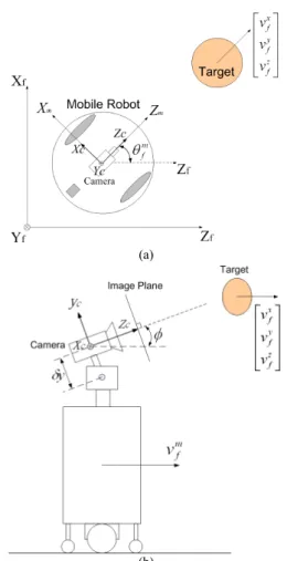
In this paper, we consider the nonholonomic visual tracking control problem such that a wheeled mobile robot with a tilt camera mounted on top of it can track a moving target. The target is supposed to be a well-recognizable object with appropriate dimensions in image plane. Fig. 1 shows an example of the scenario. A tilt camera is mounted on the mobile robot and its

opti-Chi-Yi Tsai and Kai-Tai Song

Department of Electrical and Control Engineering, National Chiao Tung University

1001 Ta Hsueh Road, Hsinchu, Taiwan, R. O. C. e-mail: chiyi.ece91g@nctu.edu.tw; ktsong@mail.nctu.edu.tw

Robust Tracking Control of a Mobile Robot

with a Tilt Camera

2 the model of the wheeled mobile robot and target in the world coordinate frame F , in which the motion of the _f target is supposed to be holonomic. Fig. 1 (b) is the side view of the scenario under consideration, in which the tilt angle

φ

is the relationship between camera coordinate frame F and the mobile coordinate frame _c F . The m

kinematics of the wheeled mobile robot and the target can be described, respectively, by m f m f m f m f m f m f m f m f w v x v z = = = θ θ θ & & & sin cos , 0 = = m f m t y w & & φ _and y f t f x f t f z f t f v y v x v z = = = & & & (1) where ( , , m) f m f m f x y z and ( , , t) f t f t f x y

z are, respectively, the positions of the mobile robot and the target in Cartesian coordinates. ₍θm_,φ₎

f are the orientation angle of the

mo-bile robot and the tilt angle of the camera. ( , m)

f m

f w

v are

the linear and angular velocity of the mobile robot. m t

w denotes the tilt velocity of the camera. ( , , y)

f x f z f v v v are the

target velocity in Cartesian coordinates.

Fig. 2 shows the relationship between the world, camera and image coordinate frames. In Fig. 2,

) , ,

(x_c y_c z_c are the target coordinates with respect to robot coordinates in the camera coordinate frame such that

X m f t f m f c =R(φ,θ )(X −X )−R(φ)δ X , (2) where ⎥ ⎥ ⎥ ⎦ ⎤ ⎢ ⎢ ⎢ ⎣ ⎡ − − − = m f m f m f m f m f m f m f R θ φ φ θ φ θ φ φ θ φ θ θ θ φ cos cos sin sin cos cos sin cos sin sin sin 0 cos ) , ( , ⎥ ⎥ ⎥ ⎦ ⎤ ⎢ ⎢ ⎢ ⎣ ⎡ = c c c c z y x X , ⎥ ⎥ ⎥ ⎦ ⎤ ⎢ ⎢ ⎢ ⎣ ⎡ = t f t f t f t f z y x X , ⎥ ⎥ ⎥ ⎦ ⎤ ⎢ ⎢ ⎢ ⎣ ⎡ = m f m f m f m f z y x X , ⎥ ⎥ ⎥ ⎦ ⎤ ⎢ ⎢ ⎢ ⎣ ⎡ − = φ δ φ δ δ sin cos 0 y y X and

δ

y

is the

distance between the center of robot head and the camera. Because _{R(φ)δX =}

[

_{0 δy 0}

]

T _{is a constant translation}

vector, the derivative of (2) becomes

) )( , ( ) ( ) , ( ) , ( m f t f m f m f t f m f m f m f m f c X X X X

X& & & − + & − & ⎥ ⎥ ⎦ ⎤ ⎢ ⎢ ⎣ ⎡ ∂ ∂ + ∂ ∂ = θ φθ θ θ φ φ φ θ φ R R R , (3) where ) , ( ) , ( 1 m f m f φ φθ θ φ ΨR R ∂ = ∂ , ( , ) ( , m) f m f m f θ φθ θ φ ΨφR R ∂ = ∂ , ⎥ ⎥ ⎥ ⎦ ⎤ ⎢ ⎢ ⎢ ⎣ ⎡ − = 0 1 0 1 0 0 0 0 0 1 Ψ , ⎥ ⎥ ⎥ ⎦ ⎤ ⎢ ⎢ ⎢ ⎣ ⎡ − − = 0 0 cos 0 0 sin cos sin 0 φ φ φ φ φ Ψ .

Substituting (1) and (2) into (3), the kinematics of the interaction between the robot and the target in camera frame is obtained such that

t f m f c c c c =A X +Bu+R(

φ

,

θ

)V X& , (4) where ⎥ ⎥ ⎥ ⎦ ⎤ ⎢ ⎢ ⎢ ⎣ ⎡ − − − = 0 cos 0 sin cos sin 0 t f m f t f m f m f m f c w w w w w w φ φ φ φ A , (a) (b)

Fig. 1. (a) Model of the wheeled mobile robot and target in the world coordinate frame. (b) Side view of the wheeled mobile robot with a tilt camera mounted on its head to track a dynamic target.

Fig. 2. Relationship between coordinate systems, world, camera and image coordinate frames.

⎥ ⎥ ⎥ ⎦ ⎤ ⎢ ⎢ ⎢ ⎣ ⎡ − = y y c δ φ φ φ δ 0 cos 0 0 sin 0 sin 0 B , ⎥ ⎥ ⎥ ⎦ ⎤ ⎢ ⎢ ⎢ ⎣ ⎡ = t f m f m f w w v u , ⎥ ⎥ ⎥ ⎦ ⎤ ⎢ ⎢ ⎢ ⎣ ⎡ = z f y f x f h v v v V .

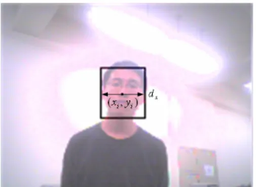
Next, we define the system states in image frame for controller design. Fig. 3 illustrates the definition of ob-served system states in image plane. By the definition of the diffeomorphism on an image plane:

[

]

[

]

T x c y c x T x i i i x y d k x k y k X = = − W , k_x=f_x z_c , c y y z

zontal and vertical position of the centroid of target in image plane; d_x is the width of target in image plane;

) f , f

( x y represent the fixed focal length along the image

x-axis and y-axis, respectively [10]; W denotes the width

of the target. Using direct computation, the kinematic interaction between robot and target in image frame can be obtained by taking the derivative of theexpression in diffeomorphism such that

i i i i i X u C X& =A +B + , (5) where A_i =diag(A₁,A₂,A₁), ) cos cos sin sin cos ( f 1 m f z f y f m f x f x x _{v v v} k A =− φ θ + φ+ φ θ , ) cos cos sin sin cos ( f 2 m f z f y f m f x f y y _{v v v} k A =− φ θ + φ+ φ θ , ⎥ ⎥ ⎥ ⎥ ⎥ ⎥ ⎥ ⎥ ⎦ ⎤ ⎢ ⎢ ⎢ ⎢ ⎢ ⎢ ⎢ ⎢ ⎣ ⎡ + − + + − + + + − + − + = y i y x x x i i x x y i y y i y i i x y y i y y i y i i y y x x x i i x x i y y k d d x d k y y k y y x y k y y k x y y k x x k f ) ( cos f cos f f f ) cos f (sin f f ) cos f (sin f ) ( sin ) ( f f cos ) f f ( cos f 2 2 2 2 δ φ φ δ φ φ φ φ δ φ δ φ φ B , ⎥ ⎥ ⎥ ⎦ ⎤ ⎢ ⎢ ⎢ ⎣ ⎡ − − − = 0 ) cos sin sin sin cos ( ) cos sin ( m f z h m f x h y h y m f x h m f z h x i k v v v v v k C φ φ θ φ θ θ θ , ) , , (abc

diag denotes a 3-by-3 diagonal matrix with

di-agonal element a, b, and c. We observe that the kine-matics of the interaction between the mobile robot and the target in image frame can be modeled as a linear time-varying (LTV) system, in which the system state is

[

]

T

x i

i y d

x and the control signal is

[

m

]

T t m f m f w w v .

In order to control the system state from an initial state to a desired state, we transform the system model into an error-state model. First, define the error coordinates in image plane such that

[

]

[

]

T x x i i i i T e e e e x y d x y d X = = x − y − d − , (6) where

[

]

T x i i f

X = x y d is the fixed desired state in image plane. Second, the dynamic error-state model in image plane can be derived directly by taking the de-rivative of (6). The result is given by

) ( i f i i e i e X u X C X& =A −B − A + . (7) With the new coordinates

[

]

T

e e

e y d

x , the visual

track-ing control problem is transformed into a stability prob-lem. If (x_e,y_e,d_e) converges to zero, then the visual tracking control problem is solved.

III.VISUAL TRACKING CONTROLLER

In this section, a tracking control law based on the proposed error-state model (7) for tracking a static or moving target in image plane is derived exploiting the conventional pole placement approach. First, we choose the feedback control law such that

) ( 1 i f i e i X X C u=_B− _K −_A − _{, (8)}

Fig. 3. The definition of observed system states in image plane.

) β ρ , β ρ , β ρ ( _{1 1} A_{1 2 2} A_{2 3 3} A₁ diag + + + = K ,

in which (ρ1,ρ2,ρ3) are three fixed positive scalar factors,

and (β1,β2,β3) are three positive constants. Substituting

(8) into (7) yields e e i e X diag X X& =(A −K) =− (ρ1β1,ρ2β2,ρ3β3) . (9) Because (ρ1,ρ2,ρ3,β1,β2,β3)>0 are positive constants,

the error-state X_e(t) will decay exponentially to zero. It is clear that the system is asymptotically stable and the visual tracking control problem is solved.

Note that the feedback control law (8) poses a singu-larity problem in matrix B_i. By direct computing, the singularity condition of matrix B_i (detB_i =0) can be found such that

φ tan ) S ( f_y = y_i+ d_x , (10) where S=(fyδy)/(fxW) is a fixed scalar factor. In other

words, if expression (10) is satisfied, then the determinant of matrix B_i will become zero and matrix Bi will

be-come singular. Therefore, expression (10) plays an im-portant role for us to predict the singularity of matrix B_i. More specifically, define a singularity index (SI) such that φ tan ) S ( f_y y_i d_x SI= − + . (11) If SI is smaller than a preset threshold value, we then need to switch to another controller, such as a PID controller, instead of using the proposed one.

Summarizing the above discussions, we obtain the following theorem.

Theorem 1: Suppose the initial position of user’s face is in the camera field-of-view. Let (ρ₁,ρ₂,ρ₃)>0be three fixed positive scalar factors and (β1,β2,β3)>0be three

positive constants. Consider the linear time-varying (LTV) system (5). If the matrix B_i is nonsingular, then the face tracking interaction control problem can be solved using control law

) ( 1 i f i e i X X C u=_B− _K −_A − _{, (12)} where A_i, B_i and C_i are defined in (5). X and _e Xf are

defined in (6). K is a 3-by-3 diagonal matrix such that ) β ρ , β ρ , β ρ ( 1 1 A1 2 2 A2 3 3 A1 diag + + + = K ,

4 in which (A1,A2) are defined in (5).

IV. ROBUSTNESS ANALYSIS

In this section, we investigate the robustness of pro-posed visual tracking controller (12) against the model uncertainties on camera, robot and target parameters. We first define a positive-definite Lyapunov function

) ( 2 1 ) , , ( 2 2 2 e e e e e e y d x y d x V = + + . (13)

Taking the derivative of (13) yields

) ( ] ) ( [X X C X u f u X X V i T e i i i T e e T e =− + + ≡− = & A B & . (14)

In view of Lyapunov theory [11], expression (14) tells us that if f(u)>0 then the equilibrium point of (7) is as-ymptotically stable. Consider the following LTV system with parametric uncertainties:

)] ( ) [( ) ( ) ( ) ( i i f i i i i e i i i f i i e i e C C X u X C X u X X δ δ δ δ − + − + + + + = + − − = A A B B A A A B A & (15) where δA_i=diag(δA₁,δA₂,δA₁) is an unknown bounded

diagonal-matrix-disturbances; δB_i is an unknown

bounded matrix-disturbances; δC_i is an unknown bounded vector-disturbances. Hence, the derivative of (13) with parametric uncertainties becomes

) ( )] ( ) ( [ ] ) ( [X X C X u f u f u f u V T _i e i i i T e + + =− + ≡− − = A B δ & _, (16) where δf(u)=XeT(δAiXi+δCi)+XeTδBiu is unknown. Without loss of generality, let us assume that X_e and u are both bounded vectors. This implies that δf(u) is bounded and there exist a positive definite matrix Q~ such that e T e X X u f( )< Q~ δ , (17)

where Q~=diag(δ₁,δ₂,δ₃)>0; (δ1,δ2,δ3) are three posi-tive unknown upper-bound associated with error-states

) , ,

(xe ye de , respectively. From (21) and (22), it follows that ) ( ~ ) (u X X f u f e T e < − Q . (18)

Expression (18) implies that T _e

e X X u f( )− Q~ is a lower-bound of f(u) . If ( )− T~ _e>0 e X X u f Q can be

guaranteed, then f(u)>0 is satisfied and thus the sys-tem has the robust property w.r.t. the parametric uncer-tainties.

Choose the controller u as in (12) with parametric uncertainties such that

) ( 1 i f i e i X X C u=_B− _K −_A − _{, (19)} where Kg=diag(ρ1β1+A1,ρ2β2+A2,ρ3β3+A1); (A1,A2,A1)

are the diagonal elements of matrix A . Substituting (19) _i into (16) yields e T e e i g T e X X X X u f V& =− ( )=−[ (K −A) ]≡− Q , (20) where Q=K_g−A_i=diag(ρ₁β₁,ρ₂β₂,ρ₃β₃)>0 is a constant

positive definite matrix. From (18) and (20), it is clear that ) ( ) ~ ( ~ ) (u X X X X f u f e T e e T e = − < − Q Q Q , (21)

where Q−Q~=diag(ρ1β1−δ1,ρ2β2−δ2,ρ3β3−δ3).

Expres-sion (21) tells us that if the parameters (ρ1β1,ρ2β2,ρ3β3) are, respectively, larger than the unknown upper-bound

) , ,

(

δ

₁

δ

₂

δ

₃ defined in (22), then Q−Q~ becomes a posi-tive definite matrix and thus f(u)−XeTQ~Xe>0 is satis-fied, which means the proposed visual tracking controller (12) is robust against the unknown parametric uncertain-ties. Therefore, summarize the above discussions, we obtain the following theorem.

Theorem 2: Consider the LTV system (5) with unknown bounded parametric uncertainties δ , A_i δ and Bi δ de-Ci

fined in (15). Let (

δ

₁,

δ

₂,

δ

₃) be three positive up-per-bound defined in (17). Choose the controller u as in the expression (12) with parameters (ρ₁,ρ₂,ρ₃)> and 0

0 ) β , β , β

( 1 2 3 > . Then, the closed-loop visual tracking system is asymptotically stable for all ρ₁β₁>δ₁ ,

2 2 2β

ρ > and δ ρ₃β₃ >δ₃.

V. EXPERIMENTAL RESULTS

Fig. 4 shows two experimental mobile robots devel-oped in the intelligent system control integration (ISCI) Lab, NCTU. Left robot is equipped with a USB camera and tilt platform to track another robot on which a target of interesting was installed. In realization of the control schemes, it was noted that the quantization error in ve-locity commands degrade the performance of the con-troller and might make the system unstable. In order to eliminating the velocity quantization error encountered in practical system, we combined a robust control law pre-sented in authors’ previous work [12] with the proposed visual tracking controller. Table I tabulates the parame-ters used in the experiment.

A. Visual Tracking Control Experiment

In this experiment, the wheel velocities and the initial pose of the target robot are set as ( , t)=(12cm/s ,9cm/s)

l t r v

v

and (140cm ,30cm, π), respectively. This means that the

target would move along a counterclockwise circular path. The initial pose of the tracking robot is (0cm ,0cm ,0).

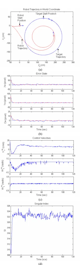
Fig. 5 presents the recorded responses of this experiment. In Fig. 5(a), the robot trajectories were recorded in world coordinates. Because these two robots were face to face in initial state, the tracking robot first moved backward in the beginning and then moved forward to track the target robot. We see that the tracking robot tracked the target robot successfully in a circular motion. These experi-mental results verify the performance of the proposed visual tracking controller and robust control law. Fig. 5(b) depicts the tracking errors in image plane. In Fig. 5(b),

Fig. 4. Two experimental mobile robots Table 1. Parameters used in the experiment

Symbol Quantity Description W 12 cm Width of the target D 40 cm Distance between two _{drive wheels}

) f , f

( x y (294,312) pixels Focal lengths of camera _{in retinal coordinates}

) d , y , x

( _{i i x} (0, 0, 35) Desired state in image plane

) ρ , ρ , ρ

( _{1 2 3} (1/16,1/8,1/16) Three scalar factors ) β , β , β

( 1 2 3 (5,6,4) Three positive constants

the dotted lines illustrate the theoretical result from (9) while the solid lines show the experimental results of tracking errors. We observe that the system state in the experiment converges to the desired state as expected. Fig. 5(c) shows the linear and angular velocities of tracking robot’s centre point. It reveals that the tracking robot’s linear and angular velocities converge to con-stants when the tracking errors decay to zero. Therefore, the tracking robot kept tracking the target robot con-tinuously. Fig. 5(d) illustrates the response of SI value from (11) in the experiment. It shows that the SI value is large enough at every moment, and the matrix B is _i nonsingular during the visual tracking procedure.

B. Extension of the Proposed Method

The visual tracking controller proposed in this paper can be extended to several applications of engineering interest, e.g., wheeled mobile robot motion control for human-robot interaction. In the authors’ previous work [13], the proposed visual tracking controller was com-bined with a real-time face detection and tracking algo-rithm to control the mobile robot to efficiently interact with the human motion for vision-based human-robot interaction.Fig. 6 shows photos of motion sequences of visual interaction between human and the robot during the visual tracking experiment. In Fig. 6(a), the tracking robot detected the user’s face and started visual tracking interaction. In Figs. 6(b) and (c), the tracking robot moved forward automatically to track the user’s face. In Fig. 6(d), the tracking robot tracked the user successfully and stopped moving forward.

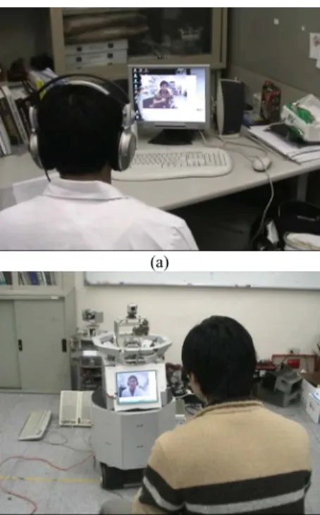
Another application of the proposed visual tracking controller was combined with wireless LAN video and speech communication techniques to implement remote

(a)

(b)

(c)

(d)

Fig. 5. Experimental results. (a) Robot trajectory in world coordinates. (b) Tracking errors in image plane. (c) Control velocities of the center point and tilt camera of tracking robot. (d) Transition of singular index (11) in every moment.

6 (a)

(b)

Fig. 6 Recorded image sequence of human-robot interaction control.

(a)

(b)

Fig. 7 Remote consulting by video and speech communication via wireless LAN. (a) Remote computer (the doctor side) (b) Healthcare robot (the patient side)

consulting function for healthcare robot. Fig. 7 shows the demonstration of remote consulting function. Figs. 7(a) and 7(b) are the picture of remote computer (the doctor side) and healthcare robot (the patient side), respectively. Using this function, the doctor can communicate with the patient directly via the healthcare robot to examine the patient’s health remotely.

VI. CONCLUSION

In this paper, a new visual interaction control model that represents the relationship between a mobile robot and a moving object in image plane has been derived.

Based on this model, a single visual tracking controller has been proposed to effectively resolve visual tracking control design of both static and moving targets with asymptotical convergence. In robustness analysis, we have shown that the proposed visual tracking controller is robust w.r.t. some uncertainties in the model. Experi-mental results validate that the proposed control schemes guarantee asymptotic stability of the visual tracking sys-tem. The proposed controller can be extended to several applications of engineering interest. The proposed con-trol scheme provides a useful solution for visual tracking control of wheeled mobile robots to track a target of in-teresting effectively and interactively.

ACKNOWLEDGMENT

The authors would like to thank Prof. Ti-Chung Lee for his suggestion for the system modeling in this study. This work was supported by the National Science Coun-cil of Taiwan, ROC under grant NSC 94-2218-E-009-008.

REFERENCES

[1] G. López-Nicolás, C. Sagüés, J.J. Guerrero, D. Kragic and P. Jensfelt, “Nonholonomic epipolar visual servoing,” in Proc.

IEEE Intl. Conf. on Rob. and Auto., Orlando, Florida, USA, pp. 2378-2384, 2006.

[2] A. Suluh, K. Mundhra, T. Sugar, and M. McBeath, “Spatial interception for mobile robots,” in Proc. IEEE Intl. Conf. on Rob.

and Auto., Washington, DC, USA, pp. 4263-4268, 2002. [3] A. K. Das, R. Fierro, V. Kumar, J. P. Ostrowski, J. Spletzer, and C.

J. Taylor, “A vision-based formation control framework,” IEEE

Trans. on Rob. And Auto., Vol. 18, No. 5, pp. 813-825, 2002. [4] H. Zhang and J. P. Ostrowski, “Visual servoing with dynamics:

control of an unmanned blimp,” in Proc. IEEE Intl. Conf. on Rob.

and Auto., Detroit, Michigan, USA, pp. 618-623, 1999. [5] F. Conticelli, B. Allotta, and P. K. Khosla, “Image-based visual

servoing of nonholonomic mobile robots,” in Proc. IEEE 38th

Conf. Decision Contr., Phoenix, Arizona, USA, pp. 3496-3501, 1999.

[6] J. P. Barreto, J. Batista, H. Araújo, and A. T. Almeida, “Control issues to improve visual control of motion: applications in active tracking of moving targets,” in Proc.AMC00-IEEE/RSJ Intl. Workshop on Advanced Motion Control, Japan, 2000, pp. 13-18. [7] D. Burschka, J. Geiman, and G. Hager, “Optimal landmark con-figuration for vision-based control of mobile robot,” in Proc.

IEEE Intl. Conf. on Rob. and Auto., Taipei, Taiwan, 2003, pp. 3917-3922.

[8] H. Y. Wang, S. Itani, T. Fukao and N. Adachi, “Image-based visual adaptive tracking control of nonholonomic mobile robots,” in Proc. IEEE Intl. Conf. on Intelligent Rob. and Sys., Maui, Hawaii, USA, pp. 1-6, 2001.

[9] J. Chen, W. E. Dixon, D. M. Dawson, and M. McIntyre, “Ho-mography-based visual servo tracking control of a wheeled mo-bile robot,” IEEE Trans. on Rob., Vol. 22, No. 2, pp. 407-416, 2006.

[10] A. Habed and B. Boufama, “Camera self-calibration: a new ap-proach for solving the modulus constraint,” in Proc. IEEE Intl.

Conf. on Pat. Rec., Cambridge, UK, 2004, pp. 116-119. [11] J.-J. E. Slotine and W. Li, Applied Nonlinear Control.

Engle-wood Cliffs, NJ: Prentice-Hall, 1991.

[12] C.-Y. Tsai and K.-T. Song, “Robust Visual Tracking Control of Mobile Robots Based on an Error Model in Image Plane,” in Proc.

IEEE Intl. Conf. on Mech. and Auto., Niagara Falls, Canada, pp. 1218-1223, 2005.

[13] C. Y. Tsai and K. T. Song, “Face Tracking Interaction Control of a Nonholonomic Mobile Robot,” in Proc. IEEE/SRJ Int. Conf. on