以天花板上多環場攝影機輔助自動車作室內安全監控之研究

(1)

國

立

交

通

大

學

多媒體工程研究所

碩

士

論

文

以天花板上多環場攝影機輔助自動車

作室內安全監控之研究

A Study on Indoor Security Surveillance by

Vision-based Autonomous Vehicle With

Omni-cameras on House Ceiling

研究生：王建元

指導教授：蔡文祥教授

(2)

以天花板上多環場攝影機輔助自動車

作室內安全監控之研究

A Study on Indoor Security Surveillance by

Vision-based Autonomous Vehicle With

Omni-cameras on House Ceiling

研究生：王建元 Student：Jian-Yuan Wang

指導教授：蔡文祥 Advisor：Prof. Wen-Hsiang Tsai

國立交通大學

多媒體工程研究所

碩士論文

A Thesis

Submitted to Institute of MultimediaEngineering College of Computer Science

National Chiao Tung University in partial Fulfillment of the Requirements

for the Degree of Master

in

Computer Science

June 2009

Hsinchu, Taiwan, Republic of China

(3)

以天花板上多環場攝影機輔助自動車

作室內安全監控之研究

研究生：王建元指導教授：蔡文祥教授

國立交通大學多媒體工程研究所

摘要

本論文提出了一個以天花板上多環場攝影機輔助自動車做室內安全監控之方法。我們使用一部以無線網路傳遞控制訊號之自動車，並在其上裝置一部攝影機，用以監視室內環境及拍攝入侵者影像。另外使用兩部裝置在天花板上的魚眼攝影機協助此自動車做導航。在此研究中，我們提出了一種即時對環境中空地和障礙物做定位的技術，並以計算出的位置建立完整的環境地圖及規劃自動車的巡邏路線，使自動車可以在複雜的環境中導航並避開障礙物和牆壁。此外，我們亦提出了一種能夠適應高度變化的空間對映法，利用推導出的公式計算設置在不同高度的魚眼攝影機的對映表，以此對映表配合內插法，為環境中的物體進行定位。因為自動車行走時會產生機械誤差，我們也提出了四個策略，以修正自動車的位置及方向。此外，我們亦提出了一種追蹤入侵者的技術，使用追踨視窗準確地預測及計算人物在扭曲影像中的位置，並在追踨過程中同時記錄人物的特徵。為了擴大可監視的範圍，我們使用了多台裝置於天花板上的攝影機，為此我們也提出了一種在多台攝影機下“交棒” (handoff)的技術，使自動車或入侵者從一台攝影機的視野範圍移動到另外一台時，能夠不間斷的被追蹤。實驗結果證明我們所提出的方法是可行而且有效的。

(4)

A Study on Indoor Security Surveillance by Vision-based

Autonomous Vehicles with Omni-cameras on House Ceilings

Student: Jian-Yuan Wang Advisor: Prof. Wen-Hsiang Tsai, Ph. D.

Institute of MultimediaEngineering, College of Computer Science National Chiao Tung University

ABSTRACT

Vision-based methods for security surveillance using an autonomous vehicle with fixed fish-eye cameras on ceilings in an indoor environment are proposed. An autonomous vehicle controllable by wireless communication and equipped with a camera is used as a test bed and navigates in a room space under the surveillance of multiple fisheye cameras affixed on the ceiling. To learn the information of the unknown room environment in advance, a method is proposed for locating the ground regions, identifying the positions of obstacles, and planning the patrolling paths. The data obtained by the method enable the vehicle to navigate in the complicated room space without collisions with obstacles and walls. Also, a height-adaptive space mapping method is proposed, in which the coordinates of corresponding points in 2-D images and 3-D global spaces are computed by interpolation to form a space mapping table for object localization. Appropriate equations are derived to adapt the table to fish-eye cameras affixed to different ceiling heights. Because the vehicle suffers from mechanic errors, a vehicle location and direction correction method is proposed for correcting the errors according to four strategies. Furthermore, a method for detecting

(5)

be predicted first, and the exact position is then calculated via a tracking window in images. Some useful features of the intruding person are computed for person identification. To enlarge the area under surveillance using multiple cameras, the camera handoff problem is also solved by using information of the overlapping regions of the cameras’ fields of view. Experiments for measuring the precisions of the proposed methods and tracking intruding persons were conducted with good results proving the feasibility of the proposed methods.

(6)

ACKNOWLEDGEMENTS

The author is in hearty appreciation of the continuous guidance, discussions, support, and encouragement received from my advisor, Dr. Wen-Hsiang Tsai, not only in the development of this thesis, but also in every aspect of his personal growth.

Thanks are due to Mr. Chih-Jen Wu, Mr. Che-Wei Lee, Mr. Guo-Feng Yang, Miss Mei-Fen Chen, Mr. Yi-Chen Lai, Miss Chiao-Chun Huang, Miss Shu-Hung Hung, Miss Chin-Ting Yang, and Mr. Chun-Pei Chang for their valuable discussions, suggestions, and encouragement. Appreciation is also given to the colleagues of the Computer Vision Laboratory in the Institute of Computer Science and Engineering at National Chiao Tung University for their suggestions and help during his thesis study.

Finally, the author also extends his profound thanks to his family for their lasting love, care, and encouragement. He dedicates this dissertation to his beloved parents.

(7)

LIST OF FIGURES

Figure 1.1 The flowchart of proposed system. ... 7

Figure 2.1 The vehicle used in this study is equipped with a camera. (a) A perspective view of the vehicle. (b) A front view of the vehicle. ... 10

Figure 2.2 The camera system used in this study. (a) A perspective view of the camera. (b) A front view of the camera. ... 11

Figure 2.3 An Axis 207MW camera is affixed on the ceiling. ... 11

Figure 2.4 A notebook is used as the central computer. ... 12

Figure 2.5 The wireless network equipments. (a) A wireless access point. (b) A WiBox made by Lantronix. ... 12

Figure 3.1 The calibration board used for basic table construction with 15 horizontal lines and 15 vertical lines. ... 18

Figure 3.2 Finding the intersection points in the image of the calibration board. ... 19

Figure 3.3 The mapping of the origins of the ICS and GCS. ... 19

Figure 3.4 Calculating the coordinates of intersection points in the GCS by Wcali. .... 20

Figure 3.5 Calculating the coordinates of a non-intersection point by interpolation... 21

Figure 3.6 Calculating the coordinates of intersection points in the GCS by Wreal. .... 23

Figure 3.7 The imaging process of an object O1. ... 24

Figure 3.8 The imaging process of object O2. ... 25

Figure 3.9 An Image of a specific target board on the ground seen from the first camera. ... 28

Figure 3.10 The position of the target board on the ground seen from the second camera. ... 28

Figure 3.11 Calculating the vectors of the centers. ... 30

Figure 3.12  is the angle between the centerline of two images. ... 30

Figure 3.13 Calculating the adaptive mapping table of camera 2. ... 31

Figure 3.14 Calculating the global coordinates of points in the GCS. ... 32

Figure 4.1 Illustration of calculation of the similarity degree between two image points. ... 37

Figure 4.2 An example of finding the region of the ground. ... 39

Figure 4.3 An example of refining a map. (a) A rough map. (b) A complete map after applying the erosion and dilation operations. ... 41

Figure 4.4 Illustration of computing turning points to construct a new path (composed by blue line segment) different from original straight path (red line segment). ... 42

(10)

some obstacles on it. (b) The calculated new path but still some obstacles on its sub-path. (c) Repeat the algorithm to the sub-path. (d) The

calculated final path. ... 44

Figure 4.6 Steps of correcting the position of vehicle. ... 47

Figure 4.7 The calculating region. (a) with a fixed square mask. (b) with a changeable mask. ... 48

Figure 4.8 Finding the central point of a vehicle. (a) the background image of an environment. (b) The foreground image with a vehicle. (c) The found central point of a vehicle. ... 49

Figure 4.9 Using two consecutive positions to calculate the vector of direction. ... 50

Figure 4.10 False direction caused by the error of finding center. ... 52

Figure 4.11 Separating the path into two segments. ... 54

Figure 4.12 An example of avoiding dynamic obstacles. (a) The background image of an environment. (b) The image with a person stands in the environment. (c) The region of the person is found. (d) A new path is planned to avoid the dynamic obstacle. ... 56

Figure 4.13 Line L separates the region of two cameras. ... 57

Figure 5.1 The rotational invariance property. (a) A real example. (b) A vertical sketch chart... 61

Figure 5.2 Finding the positions of a person. (a)(b)(c) The person stands at several different places in an image. (d) The person stands at the center point in an image. ... 62

Figure 5.3 Prediction of the position of a person. ... 63

Figure 5.4 An example of distortion in the image taken by a fisheye camera. ... 64

Figure 5.5 Calculating p and q. ... 65

Figure 5.6 Situation 1. ... 66

Figure 5.9 An example of hand-off when a person moves from P1 to P2. ... 69

Figure 5.10 The trail of the intruding person drawn on the map. ... 71

Figure 6.1 The camera is affixed at 20 cm from the calibration board. ... 74

Figure 6.6 Finding the position of a person in the image. ... 78

Figure 6.7 The experimental positions of the person. ... 78 Figure 6.8 A real example of following the specific person. (a) The vehicle patrolled

(11)

in the laboratory. (b) through (f) The vehicle followed the person

continuously. ... 80 Figure 6.9 The images taken by the cameras on the ceiling, and the positions of the

person are indicated. ... 81 Figure 6.10 The monitored points selected by a user. ... 82

(12)

LIST OF TABLES

Table 5.1 The record of a person’s trail. ... 70

Table 6.1 The results of calculating the value of Wreal by two ways. ... 77

Table 6.2 Calculating errors of the position of a person. ... 79

Table 6.3 Records of the uncorrected mechanic errors in every segment of path ... 83

(13)

Chapter 1 Introduction

1.1 Motivation of Study

As the technology is progressing nowadays, more and more robots emerge in many applications. An autonomous vehicle is an important and common form of robots. It can move and turn by the control of programs and can take images by cameras equipped on it to increase its abilities. It is convenient to use autonomous vehicles to substitute for human beings in many automation applications. For example, a vehicle may be utilized to patrol in an environment for a long time without a rest. In addition, the video which is taken by a camera can be recorded forever for later search for its contents of various interests. For example, if a certain object in a video-monitored house is stolen, the video can be watched to find out possibly the thief, providing a better evidence of the crime than just the memory of a person.

Using vehicles to patrol in indoor environments automatically is convenient and can save manpower. The images which are taken by the cameras on vehicles may be transmitted by wireless networks to a central surveillance center, so that a guard there can monitor the environment without going to the spots of events, and this is also safer for a guard to avoid conflicts with invaders. Additionally, it is useful for a vehicle to follow a suspicious person who breaks into an indoor environment under automatic video surveillance, and clearer images of the person’s behavior can be

(14)

taken by the cameras on the vehicle. It is desired to investigate possible problems raised in achieving the previously-mentioned goals and to offer solutions to them. Possible problems include:

1. constructing the mapping tables of cameras automatically, so that the positions of vehicles, invading persons, concerned objects, etc. can be computed;

2. detection of concerned objects and humans from images acquired by cameras equipped on vehicles and/or affixed to walls or ceilings;

3. recording of invaders’ trajectories and computation of their walking speeds for later inspection for the security purpose.

We try to solve in this study all these problems for indoor environments with complicated object arrangements in space. But if the environment under surveillance is very large, we cannot monitor the entire environment by using just one omni-camera. So it is desired to use simultaneously several cameras affixed on ceilings to cover large environment areas. In order to achieve this goal, possible problems to be solved include:

1. calculating the relative positions of the omni-cameras whose fields of view (FOV’s) overlap;

2. calculating the rotation angles of the omni-cameras;

3. handling with the hand-off problem among multiple cameras.

By calculating the relative positions and rotation angles of the cameras, we can calculate the position of an object in images which are taken by the cameras. And when a person walks from one region covered by a camera to another region covered by another camera, the system should know which camera should be used to get the image of the person and where in the image should the person be localized. This is the

(15)

camera hand-off problem which we desire to deal with in this study.

Because omni-cameras are highly distorted and are affixed to the ceiling, they cannot monitor the whole environment clearly. On the other hand, autonomous vehicles are mobile and are suitable to remedy this shortness of cameras. Hence, we can utilize the vehicles to drive to the place where should be monitored to take clearer images of concerned objects or humans there as stronger evidences for crime investigations.

Another problem is that the FOV’s of omni-cameras are finite, and the cameras are expensive. If the indoor environment is very large, we will have to use many omni-cameras on the ceiling, as mentioned previously. But if we can utilize the cameras on vehicles to take images of the place which is out of the FOV’s of the cameras, we will not have to use a lot of omni-cameras.

Hence if we want to navigate a vehicle to some spot in the environment, we should calculate the position of the vehicle first, and then we can plan the path for a vehicle from its position to the spot. In most environments, there are a lot of obstacles in them, such as furniture and walls. In order to avoid collisions between vehicles and obstacles, we may gather the information of the environment first. The information may include the positions of still obstacles and open spaces where the vehicles can walk through. Afterward, we may integrate the information to construct an environment map for the purpose of convenience. In short, an environment map is used in obstacle avoidance and path planning in this study. If we want to drive a vehicle to a certain spot out of the FOV’s of the cameras, we should calculate the position and direction of the vehicle at any time and plan a path for the vehicle to drive to that spot. Possible problems in these applications include:

(16)

3. path planning and avoidance of still and dynamic obstacles in the path for the vehicle to navigate to its destination.

As a summary, in this study it is desired to investigate solutions to various problems involved in the following topics of indoor autonomous vehicle navigation:

1. security patrolling in indoor environments by autonomous vehicles;

2. effective integration of the omni-cameras on the ceiling and the cameras on the vehicles.

3. following a suspicious person and taking clearer images of her/him by the cameras on vehicles;

4. using the cameras on vehicles to monitor spots which are out of the FOV’s of omni-cameras and take clearer images.

1.2 Survey on Related Studies

In the study, we will use multiple omni-cameras on the ceiling to locate the position of a vehicle, so the omni-cameras should be calibrated before being used. Traditionally, the intrinsic and extrinsic parameters of the camera should be calculated in order to obtain a projection matrix for transforming points between 2-D image and 3-D global spaces [1, 2, 3]. Besides, a point-correspondence technique integrated with an image interpolation method have been proposed in recent years for object location estimation [4], but it will cause another problem, that is, the calibration data will change according to the environment where the cameras are used. In this study, we will propose a technique to solve this problem for the case of changing the height of the ceiling on which the cameras are affixed.

(17)

Autonomous vehicles in general suffer from mechanical errors, and many methods have been proposed to eliminate this kind of error. The geometric shapes of object boundaries [5, 6] or those labeled by users are utilized frequently [7, 8]. Furthermore, natural landmarks, such as house corners [9, 10] and the SIFT features of images [11], are also used to correct the position of a vehicle. In recent years, techniques of integrating laser range finders with conventional imaging devices have been proposed [12, 13]. Besides, when it is desired to find a specific object in the image, the method of color histogramming is often used [14].

The applications of autonomous vehicles emerge in many aspects, such as house cleaning robots, watchdog systems, automatic guides, etc. In Takeshita [15], a camera was equipped on the ceiling, and a user can control the vehicle to suck garbage on the ground by watching the images taken by the camera. In Yang [16], the vehicles were designed to patrol in an environment, too. He used the vectors of vehicles and obstacles to avoid collisions between them.

1.3 Overview of Proposed System

There are four main goals in this system. First, a vehicle should patrol automatically in an indoor environment whose information has been learned. Second, the vehicle should avoid static and dynamic obstacles, and third it should correct its position automatically. At last, the vehicle should follow an intruding person and take the images of the person.

In order to achieve these goals, the following steps should be done: 1. construct mapping tables for top-view cameras;

(18)

2. acquire environment information by top-view cameras; 3. detect obstacles on the path;

4. correct mechanic errors by top-view omni-cameras;

5. calculate the position of any intruder by top-view omni-cameras continually; 6. initiate the vehicle to follow the intruder and take images of him/her;

7. deal with the hand-off problem of the cameras.

Because we need to convert coordinates between the image coordinate system and the global coordinate system, we have to construct the mapping tables for the cameras we use first. Afterward, the coordinates between the multiple cameras can be transformed correctly. Because the vehicles patrol in the indoor environment, the environment information should be learned in advance. The information learned in this study includes the positions of obstacles and the open space in the environment where the vehicles can walk through. And the information will be used to build an environmental map.

When vehicles patrol in the environment whose information has been learned, the patrolling path can be checked to see if there are obstacles on the path. If so, the vehicles should avoid them automatically. Besides, the vehicles generally suffer from mechanical errors, so it needs to correct their positions and directions continuously, to avoid intolerable deviations from their correct path way.

When a person breaks into the environment, the position of a person will be calculated continually, and then the computer will give orders to guide a vehicle to follow the person. In order to expand the range of surveillance, several omni-cameras are used in the study, so the hand-off problem should be handled. The problem means briefly the need of identifying a person in an image acquired by a camera and passing the information to an image taken by another camera. Figure 1.1 shows a flowchart of

(19)

Figure 1.1 The flowchart of proposed system.

1.4 Contributions

Several contributions are made in this study, as described in the following: 1. A height adaptation method is proposed to construct the mapping tables for

omni-cameras in order to make the cameras usable at different ceiling heights. 2. An integrated space mapping method is proposed to localize objects in real space

using multiple fisheye cameras.

3. A method is proposed to solve the problem of camera hand-off in highly distorted images taken by fisheye cameras.

4. A method is proposed to gather distorted environment images taken by omni-cameras, and convert them into a flat map.

5. A method is proposed to correct dynamically errors of the position and direction of a vehicle caused by mechanical errors.

(20)

time on vehicle navigation paths.

7. A technique is proposed to calculate the position of a person according to rotational invariance property of omni-camera.

8. A method is proposed to predict the position of a person in a highly distorted image.

1.5 Thesis Organization

The remainder of this thesis is organized as follows. In Chapter 2, the hardware and processes of this system will be introduced. And in Chapter 3, the proposed method for constructing the mapping tables for fisheye cameras will be described.

In Chapter 4, the construction steps of an environmental map and the proposed method for obstacle avoidance are described, and four strategies of correcting the positions and directions of vehicles are also described. In Chapter 5, the method of finding specific partial regions in an image to compute the position of a person and the technique for prediction of the person’s next movement are described. The hand-off problem is solved in this chapter, too.

The experimental results of the study are shown in Chapter 6, and some discussions are also included. At last, conclusions and some suggestions for future works are given in Chapter 7.

(21)

Chapter 2 System Configuration

2.1 Introduction

The hardware and software which are used in this study will be introduced in this chapter. The hardware includes the autonomous vehicle we use and the fisheye cameras and wireless network equipments. The software includes the programs for the processes of gathering the information of an environment, constructing an environment map, avoiding obstacles when patrolling in an environment and calculating the position of a person automatically.

2.2 Hardware

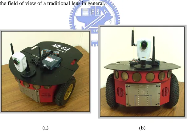
The autonomous vehicle we use in this study is aPioneer 3-DX vehicle made by MobileRobots Inc., and an Axis 207MW camera made by AXIS wasequipped on the vehicle as shown in Figure 2.1. The Axis 207MW camera is shown in Figure 2.2.

The Pioneer 3-DX vehicle has a 44cm38cm22cm aluminum body with two 19cm wheels and a caster. It can reach a speed of 1.6 meters per second on flat floors, and climb grades of 25o and sills of 2.5cm. At slower speeds it can carry payloads up to 23 kg. The payloads include additional batteries and all accessories. By three 12V

(22)

fully charged initially. A control system embedded in the vehicle makes the user’s commands able to control the vehicle to move forward or backward, or to turn around. The system can also return some status parameters of the vehicle to the user.

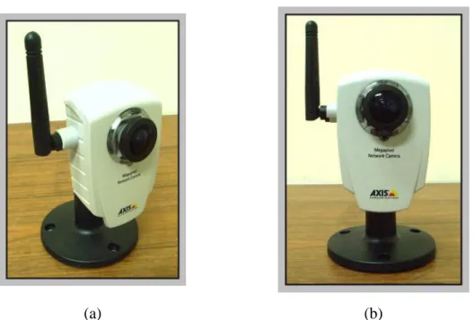
The Axis 207MW camera has the dimension of 855540mm (3.3”2.2”1.6”), not including the antenna, and the weight of 190g (0.42 lb), not including the power supply, as shown in Figure 2.4. The maximum resolution of images is up to 12801024 pixels. In our experiment, the resolution of 320240 pixels is used for the camera fixed on the vehicle and that of 640480 pixels is used for the one affixed on the ceiling. Both of their frame rates are up to 15 fps. By wireless networks (IEEE 802.11b and 802.11g), captured images can be transmitted to users at speeds up to 54 Mbit/s. Each camera used in this study is equipped with a fish-eye lens that expands the field of view of a traditional lens in general.

(a) (b)

Figure 2.1 The vehicle used in this study is equipped with a camera. (a) A perspective view of the vehicle. (b) A front view of the vehicle.

(23)

(a) (b)

Figure 2.2 The camera system used in this study. (a) A perspective view of the camera. (b) A front view of the camera.

The Axis 207MW cameras are fisheye cameras. They are also affixed on the ceiling and utilized as omni-cameras, as shown in Figure 2.3. A notebook is used as a central computer to control the processes and calculate needed parameters from the information gathered by the cameras.

(24)

Figure 2.4 A notebook is used as the central computer.

Communication between the hardware components mentioned above is via a wireless network, a WiBox made by Lantronix equipped on the vehicle, in order to deliver and receive the signals of the odometer as shown in figure 2.5.

(a) (b)

Figure 2.5 The wireless network equipments. (a) A wireless access point. (b) A WiBox made by Lantronix.

(25)

2.3 System Process

In the proposed process of constructing the mapping tables for omni-cameras, we calculate the relative positions and rotation angles between the cameras. Afterward, mapping tables are constructed automatically for every camera, and a point-correspondence technique integrated with an image interpolation method is used to calculate the position of any object appearing in the image.

In the proposed process of environment learning, the information is gathered by a region growing technique first. The information includes the position of obstacles and open spaces where a vehicle can drive through. Afterward, the positions will be converted into the global coordinate system, and an environment map will be constructed by composing the coordinates of all obstacles appearing in the vehicle navigation environment.

In the proposed process of security patrolling in an indoor environment, each vehicle is designed to avoid obstacles on the navigation path. If there are some obstacles on a path of the vehicle, the vehicle system will plan several turning points to form a new path for the vehicle to navigate safely. After the vehicle patrol for a while, it will diverge from its path because the vehicle suffers from mechanical errors. In the proposed process of vehicle path correction, we calculate the position of a vehicle in the image coordinate system by the images taken by the omni-cameras affixed on the ceiling, and then convert the coordinates into global coordinates and modify accordingly the value of the odometer in the vehicle.

In the proposed process of person following, the position of an intruding person’s feet is calculated also by the images taken by omni-cameras on the ceiling, and then

(26)

system will calculate the relative position and the rotation angle between the vehicle and the person, and adjust accordingly the orientation and speed of the vehicle to achieve the goal of following the person.

The major processes of the system are summarized and listed below: 1. Construct mapping tables for every top-view cameras.

2. Acquire environmental information by top-view cameras and construct the environment map.

3. Correct mechanic errors continuously in each cycle. 4. Plan a path to avoid obstacles in the environment.

5. Detect, predict, and compute the position of any intruding person by top-view omni-cameras continuously.

6. Handle the camera hand-off problem to keep tracking any intruding person using a single camera at a time.

(27)

Chapter 3 Adaptive Space Mapping Method for

Object Location Estimation Subject

to Camera Height Changes

3.1 Ideas of Proposed Adaptive Space

Mapping Method

In this study, we use multiple fish-eye cameras affixed on the ceiling to keep an indoor environment under surveillance. The cameras are utilized to locate and monitor the autonomous vehicle, and trace the track of any suspicious person when he/she comes into the environment. When using these omni-cameras, we want to know the conversion between the ICS (image coordinate system) and the GCS (global coordinate system). So we propose a space mapping method and construct a mapping table for converting the coordinates of the two coordinate systems.

Because the indoor environment under surveillance is unknown at first, we propose further in this study another space mapping method by which the cameras can be affixed to different ceiling heights for use, which we call height-adaptive space

mapping method. Besides, multiple fish-eye cameras are used in the mean time to

monitor an environment in this study, so calculating the relative positions and angles between every two cameras which have overlapping fields of view (FOV’s) is needed

(28)

and is done in this study. Finally, a point-correspondence technique integrated with an image interpolation method is used to convert the coordinates between the ICS and the GCS.

3.2 Construction of Mapping Table

In this section, we propose a method of constructing a basic mapping table for use at a certain ceiling height. The mapping table we use contains 1515 pairs of points, each pair including an image point and a corresponding space point. And the data of each pair of points in the table includes the coordinates (x1, y1) of the image

point in the ICS and the coordinates (x2, y2) of the corresponding space point in the

GCS. We use a calibration board which contains 15 vertical lines and 15 horizontal lines to help us constructing the mapping table.

First, we take an image of the calibration board, find the curves in the image by curve fitting, and calculate the intersection points of the lines in the image. Then, we measure manually the width of the real-space interval between every two intersection points, and compute the coordinates of the intersection points in the GCS in terms of the value of this interval width. Afterward, we affix the cameras to the ceiling, and modify the global coordinates in the mapping table by the height of the ceiling. The details of these tasks will be described in Sections 3.2.1 and 3.2.2. The major steps from constructing a space mapping table to calculating the position of a certain object are described below.

(29)

from the floor and take an image of the calibration board under the camera. Step 2. Find the curves in the image of the calibration board by curve fitting, and

calculate the coordinates of the intersection points of the curves in both the ICS and the GCS, forming a basic space mapping table.

Step 3. Attach the camera to the ceiling.

Step 4. Calculate the coordinates of the intersection points of the calibration board in the GCS utilizing the height of the ceiling assumed to be known and the content of the basic space mapping table, forming an adaptive space

mapping table.

Step 5. Calculate the relative positions and rotation angles between the cameras. Step 6. Calculate the position of any object under the camera by a

point-correspondence technique integrated with an image interpolation method using the adaptive space mapping table.

In both the basic and adaptive space mapping tables, we only record the coordinates of the corresponding intersection points between the ICS and the GCS. When we want to calculate the position of a certain object which is not right on the above-mentioned intersection points, a point-correspondence technique integrated with an image interpolation method will be applied (Step 6 above). The detail will be described in Section 3.4. We only have to calculate the coordinates in the GCS and construct the adaptive mapping table once after the cameras are attached to the ceiling (Step 4 above). The adaptive mapping table can be stored in a computer and can be used any time.

(30)

3.2.1 Proposed Method for Constructing A

Basic Mapping Table

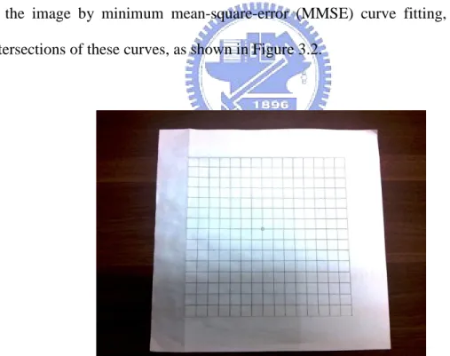
The basic mapping table of a camera should be constructed first before the camera can be used for environment monitoring. Assume that the camera is attached at a fixed height h (not necessarily to the ceiling). To construct the basic mapping table, at first we put a calibration board on the ground right under the camera. The calibration board contains at least 15 horizontal lines and 15 vertical lines, and the intervals between every two lines are all the same, as shown in Figure 3.1. Then, we use the camera to take an image of the calibration board, extract the quadratic curves in the image by minimum mean-square-error (MMSE) curve fitting, and find the intersections of these curves, as shown in Figure 3.2.

Figure 3.1 The calibration board used for basic table construction with 15 horizontal lines and 15 vertical lines.

These intersection points are described by image coordinates, which are recorded in the basic mapping table. And the height h of the camera is recorded, too. We

(31)

to the origin in the GCS, as shown in Figure 3.3.

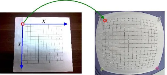
Figure 3.2 Finding the intersection points in the image of the calibration board.

Figure 3.3 The mapping of the origins of the ICS and GCS.

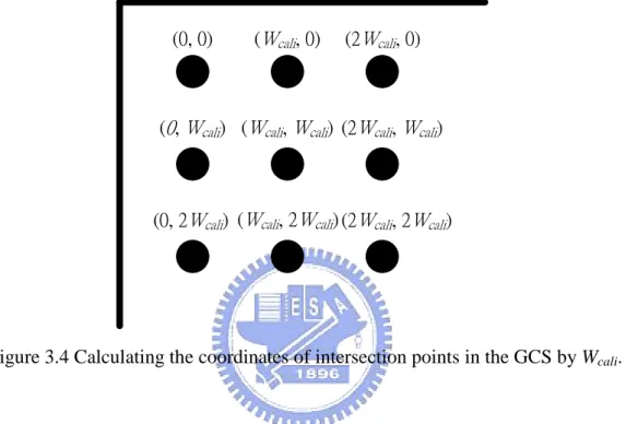
Afterward, we measure manually the width of the real-space interval Wcali between every two intersection points on the calibration board, and the global coordinates of the intersections can be calculated by the following way.

First, assume that the upmost and leftmost point in the image is just the projection of the origin of the GCS. So, the global coordinates of this point are (0, 0). The x-axis is in the horizontal direction, and the y-axis is in the vertical direction.

(32)

Hence the coordinates of the intersection points in the GCS can be calculated simply as a multiple of the value Wcali as shown in Figure 3.4. Or more specifically, the global coordinates of the (i, j)-th intersection point in Figure 3.4 may be computed as (i Wcali, j Wcali), where the origin is regarded to be the (0, 0)-th intersection point.

(0, 0) (Wcali, 0) (Wcali, Wcali) (Wcali, 2Wcali) (0, Wcali) (0, 2Wcali) (2Wcali, 0) (2Wcali, Wcali) (2Wcali, 2Wcali)

Figure 3.4 Calculating the coordinates of intersection points in the GCS by Wcali.

If the cameras are used at a height which is the same as that used during the stage of constructing the basic mapping table, we can then use this table to calculate the position of any object under the camera by a point-correspondence technique integrated with an image interpolation method, which will be described in next section.

But if the camera is used at a different height, the global coordinates in the basic mapping table should be modified. Otherwise, the object position we calculate later will be wrong. The method will be described in Section 3.2.3.

(33)

3.2.2 Using a Point-correspondence

Technique Integrated With An Image

Interpolation Method to Locate

Objects

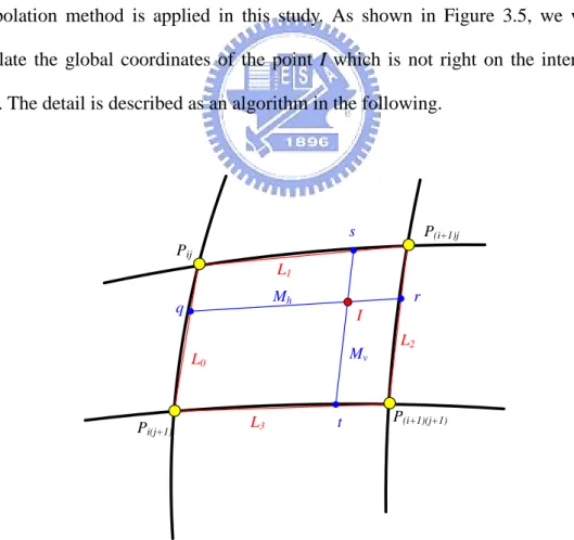
After the basic mapping table is constructed, we can know the corresponding coordinates of the above-mentioned intersection points in the ICS and the GCS. But when we want to calculate the position of a certain object which is not right on any intersection point, a point-correspondence technique integrated with an image interpolation method is applied in this study. As shown in Figure 3.5, we want to calculate the global coordinates of the point I which is not right on the intersection point. The detail is described as an algorithm in the following.

Pij Pi(j+1) P(i+1)j P(i+1)(j+1) L0 L1 L2 L3 t s r q Mh _I Mv

Figure 3.5 Calculating the coordinates of a non-intersection point by interpolation.

(34)

Input: A mapping table and the image coordinates of a non-intersection point I.

Output: The global coordinates of the space point G corresponding to I.

Steps:

Step 1. Derive the equations of the lines L0, L1, L2 and L3 in the ICS by the image

coordinate data of the points Pij, P(i+1)j, P(i+1)(j+1) and Pi(j+1), as shown in Figure 3.5.

Step 2. Derive the equations of lines Mh and Mv in the ICS.

Step 3. Calculate the image coordinates of the intersection points s, r, t, and q. Step 4. Calculate the global coordinates G of point I in the GCS.

The above algorithm is just an outline, whose details are now explained. In Step 1, the image coordinates of Pij, P(i+1)j, P(i+1)(j+1) and Pi(j+1) are known, so the equations of lines L0, L1, L2 and L3 in the ICS can be derived. In Step 2, the slope of Mh is the average of those of lines L1 and L3, and the slope of Mv is the average of those of lines

L0 and L2. The equation of Mh and Mv in the ICS can be derived by these slopes and I. Then, the intersection point s of L1 and Mv can be computed accordingly, so are r, t, and q in similar ways. Finally, the global coordinates (Gx, Gy) of I can be calculated by the following formulas according to the principle of side proportionality under the assumption that the space area enclosed by the four corners Pij, P(i+1)j, P(i+1)(j+1) and

Pi(j+1) is not too large so that the linearity inside the area holds:

) , ( ) , ( r q d I q d W X Gx   ca li ; (3.1) ) , ( ) , ( t s d I s d W Y Gy   ca li , (3.2)

(35)

and d(q, I) means that the distance between points q and I. Note that (X, Y) = (i Wcali,

j Wcali) as mentioned previously in Section 3.2.1 if Pij is the (i, j)-th intersection point in the calibration board.

3.2.3 Proposed Method for Constructing An

Adaptive Mapping Table

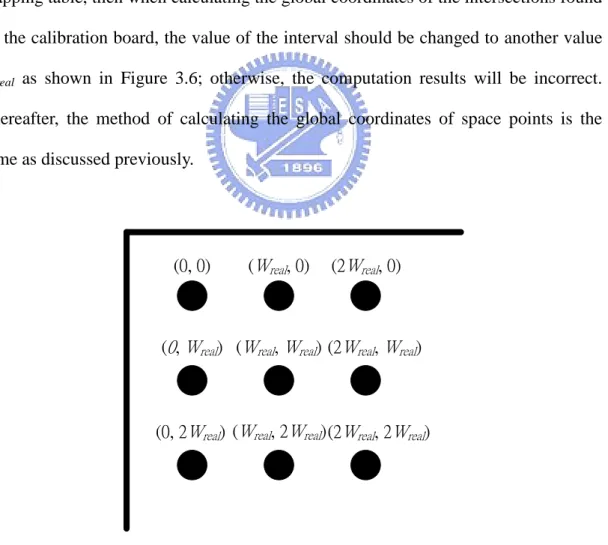
If the camera is used at a height different from that used in constructing the basic mapping table, then when calculating the global coordinates of the intersections found on the calibration board, the value of the interval should be changed to another value

Wreal as shown in Figure 3.6; otherwise, the computation results will be incorrect. Thereafter, the method of calculating the global coordinates of space points is the same as discussed previously.

(0, 0) (Wreal, 0) (Wreal, Wreal) (Wreal, 2Wreal) (0, Wreal) (0, 2Wreal) (2Wreal, 0) (2Wreal, Wreal) (2Wreal, 2Wreal)

Figure 3.6 Calculating the coordinates of intersection points in the GCS by Wreal.

(36)

attached to a lower height, the FOV’s will decrease, and the number of points found in Figure 3.2 is the same, so the value of Wreal will also decrease. On the other hand, when cameras are attached to a higher height, the FOV’s will increase, and the value of Wreal will increase, too. Accordingly, we derive a formula to calculate Wreal in the following. Note that if we use multiple cameras in this study, the global coordinates should be revised additionally, because there may be some rotation between the cameras. The detail of this problem will be described in Section 3.3.

As depicted in Figure 3.7 there is a camera lens and an object O1 with height h1

on the left. Hence, the formation of an image of O1 will be on the right side. The

distance between point B and C is d1, the distance between point C and E is f, and the

distance between E and F is a. The height of the projection of the object on the image is i. Because the two triangles ABC and CFG are similar in shape, we can obtain the following equation from the principle of side proportionality:

a f h i d   1 1 . _(3.3)

Similarly, from the similar triangles DCE and EFG, we can obtain the following equation: a f i d  1 . (3.4) B A D C E F G d1 Calibration board O1 h1 f a i Image plane

(37)

image is on the right side with height i, too. But the distance between O2 and lens is

farther than O1. The lens is the same as in Figure 3.7, and we can also obtain two

equations: b f h i d   2 2 ; _(3.5) b f i d  2 . (3.6) B A D C E F G d2 Calibration board O2 h2 f b i Image plane

Figure 3.8 The imaging process of object O2.

By Equations 3.3 and 3.4, we know

a f a f h  1 . (3.7)

By Equations 3.5 and 3.6, we know

b f b f h   2 . _(3.8) Then, we divide i d₁ by i d₂

according to Equations 3.4 and 3.6 as follows:

b f a f i d i d    2 1 (3.9) a b d d   2 1 (3.10) 2 1 d d a b   . _(3.11) We also derive 2 1 h h

(38)

b bf f a af f h h    ₂ 2 2 1 (3.12) bf f b a af f     2 ₂ . (3.13)

Substituting Equation 3.11 into the above for the value of b, we get

2 1 2 2 1 2 2 1 d d af f d d a a af f h h       (3.14) 2 1 2 1 ) ( d d a f d d a f      (3.15) b f d d a f     2 1 ) ( . (3.16)

Because the focus length of the camera does not change, and if the distance between the lens and the object image is fixed, then f + a will be equal to f + b. Hence, (3.16) leads to the following formulas:

2 1 2 1 d d h h  _(3.17) 1 1 2 2 h d h d    . (3.18)

We may rewrite the formulas above more clearly by other symbols as follows:

ca li ca li rea l rea l H W H W   . _(3.19)

where Wcali is the interval between every two intersection points on the calibration board as mentioned before; Hcali is the height between the camera and the calibration board, alse mentioned previously; Hreal is the real height at which the camera is affixed now; and Wreal is the desired new interval for use now to replace the value

(39)

3.3 Using Multi-cameras to Expand the

Range of Surveillance

Because the range of surveillance of a single camera is finite, we use multiple cameras to expand the range of surveillance in the study. First, the adaptive mapping tables should be constructed for every camera by the method mentioned above. But if there are displacements and rotations between the cameras, then the global coordinates of the mapping table should be modified further. The major steps of constructing a modified mapping table are listed below, and the detail will be described in the rest of this section.

1. Calculate the relative position of two cameras. 2. Calculate the relative rotation angle of two cameras.

3. Calculate the global coordinates of intersection points in the calibration board in the expanded range.

3.3.1 Calculating Relative Position of

Cameras

We design a special target board with a shape of a very small rhombus region on the ground as shown in Figure 3.9, and put it at the upmost and leftmost intersection area of the two cameras as shown in Figure 3.10. Because we want to calculate the global coordinates of all the intersections in the image via the coordinates of the center of this upmost and leftmost intersection area, we need to calculate the global

(40)

coordinates of this center point first.

Then, an image of the target board is taken with the first camera. The target board area in the image are found out by the information of color, and the coordinates (x, y) of the center point of the rhombus shape in the GCS are calculated by the mapping table of the first camera. Accordingly, we can know that the global coordinates of the upmost and leftmost intersection of the second camera are (x, y). More details are described as an algorithm as follows.

Figure 3.9 An Image of a specific target board on the ground seen from the first camera.

Figure 3.10 The position of the target board on the ground seen from the second camera.

(41)

Algorithm 3.2: Calculating the relative position of two cameras.

Input: An images I of a target board with a rhombus shape taken by the first

omni-camera, and the adaptive mapping table of the first camera.

Output: The global coordinates (x, y) of the center of the rhombus shape in the

upmost and leftmost intersection area of the two cameras.

Step:

Step 1. Load the image coordinates of the intersection points of the second camera, as illustrated by Figure 3.10.

Step 2. Put a specific target board on the uppermost and leftmost intersection point of the 2nd camera.

Step 3. Use the first camera to take an image of the target board.

Step 4. Calculate the central point C of the rhombus region on the target board in I taken by the first camera.

Step 5. Convert the image coordinates of C into global coordinates (x, y) by the mapping table of the first camera using Algorithm 3.1 as the desired output.

3.3.2 Calculating Relative

Rotation Angle of

Two Cameras

The relative rotation angle of the two cameras should also be calculated. In this phase we prepare two special target boards and put them on the ground. The target boards should be put on the centerline of the FOV’s of the cameras as exactly as possible. Then, the center points of the target boards in the images can be calculated, and the vectors through the center points can be obtained, as shown in Figure 3.11.

(42)

relative angle  of rotation can be calculated by the following formula: ) ( cos1 q p q p          . _(3.20) (a) (b)

Figure 3.11 Calculating the vectors of the centers.

 actually can be figured out to be the angle between the center lines (the y-axis of the ICS) of the two images as shown in Figure 3.12, and we use this value to modify the global coordinates of adaptive mapping table of the second camera.



(43)

3.3.3 Calculating Coordinates in The GCS

After the relative position and rotation angle are calculated, the adaptive mapping table of the second camera can be calculated by the following method. The black points in Figure 3.13 are represented by the global coordinates in the mapping table of camera 1, and we want to calculate the global coordinates of the blue points in the region of camera 2 to construct the adaptive mapping table of camera 2.

1 5 6 7 2 8 9 10 3 11 12 13 4 14 15 16

Camera 1

Camera 2

Figure 3.13 Calculating the adaptive mapping table of camera 2.

The coordinates (x, y), (x, y) and (x, y) in Figure 3.14 specify three blue points in Figure 3.13. The coordinates (x, y) specify any of the blue points, P1, and the

coordinates (x, y) specify another blue point Ph in the horizontal direction of P1, and

the coordinates (x, y) specify a third blue point Pv in the vertical direction of P1.

(44)

the two cameras. Both p and  are measured in advance. We can obtain four formulas to calculate (x, y) and (x, y) via (x, y) as follows:

p



(

x



,

y



) (

x



,

y



) (

x

,

y

)

P

h

P

v

P

1

Figure 3.14 Calculating the global coordinates of points in the GCS.

Horizontal:  cos 'x p x (3.21)  sin ' y p y (3.22) Vertical:  sin ' ' x p x (3.23)  cos ' ' y p y (3.24)

These four formulas are used to calculate all the global coordinates of points in the FOV of the second camera. First, the coordinates (x, y) of blue point 1 is calculated by the method described in Section 3.3.1. Then we may calculate the coordinates of blue points 2, 3 and 4 in Figure 3.13 via Equations 3.23 and 3.24 because they are on the vertical direction of P1.

(45)

p is 2Wreal, where Wreal is calculated in advance as described previously. Afterward, the horizontal points in every row are calculated by use of the points of the first column. For example, when calculating the coordinates of point 8, because this point is on the horizontal direction of point 2, Equations 3.21 and 3.22 are used and the values of x and y in them will be the coordinates of point 2, and p will be still 1Wreal. The calculating sequence is represented in Figure 3.14 by white numbers in blue circular shapes. In this way, all the coordinates of points in camera 2 can be calculated, and so the adaptive mapping table can be completed.

After all the mapping tables of every camera are constructed, we consider all the mapping tables as a combined one, and so complete the expansion of the range of surveillance.

(46)

Chapter 4 Construction of Environmental

Maps and Patrolling in Learned

Environments

4.1 Introduction

One goal of this study is to make an autonomous vehicle to patrol in an indoor environment automatically. Patrolling points where the vehicles should navigate through for security monitoring are selected by a user freely. In order to achieve this goal, an environment map should be constructed, and the vehicle should have the ability to avoid static and dynamic obstacles, or a crash may happen. Besides, autonomous vehicles usually suffer from mechanical errors, and such errors will cause the vehicle to deviate from the right path, so an automatic path correction process is needed. The process should correct the position and direction of the vehicle at appropriate timings and spots.

4.2 Construction of Environment Maps

For an autonomous vehicle to patrol in a complicated indoor environment, the environment map should be constructed first. An environment map includes a two

(47)

dimensional Boolean array in this study, and each element in the array represents a square centimeter in the global. If the value of an element in the array is true, that means there are some obstacles in this region, and the autonomous vehicle cannot go through this region. On the other hand, if the value of an element in the array is false, that means there is no obstacle in this region, and the autonomous vehicle can go through this region.

Furthermore, in this study we use multiple fish-eye cameras affixed on the ceiling to get the images of the environment, and use these images to construct the environment map. The major steps are described below.

1. Find the region of ground in taken images by a region growing technique. 2. Use the combined space mapping table to transform the image coordinates

of the ground region into global coordinates to construct a rough environment map.

3. Eliminate broken areas in the rough environment map to get the desired environment map.

More details are described subsequently.

4.2.1 Finding Region of Ground by Region

Growing Technique

A region growing method is used in this study to find the region of the ground, as mentioned previously. First, a seed is selected by a user from the ground part in the image as the start point, and the eight neighboring points of this start point are examined to check if they belongs to the region or not. The proposed scheme for this

(48)

belong to the region is used as the seed again, and the connected-component check is repeated, until no more region points can be found. More details of the method are described as an algorithm in the following.

Algorithm 4.1: Finding the region of the ground in an image.

Input: An image taken by a camera on the ceiling.

Output: The image coordinates of the region of the ground in the image.

Steps:

1 Select a seed P from the ground part in the image manually as the start point, and regard it as a ground point.

2 Check the eight neighboring points Ti of P to see if they belong to the region or not.

2.1 Find all the neighboring points Ni of Ti which belong to the region of the ground for each Ti.

2.2 Calculate the value of the similarity degree between Ti and each Ni.

2.3 Decide whether Ti belongs to the ground region according to the similarity values by the following steps.

2.3.1 Compare the values of similarity calculated in Step 2.2 with a threshold

TH1 separately (the detail will be described later).

2.3.2 Calculate the number p of similarity values which are larger than TH1.

2.3.3 Calculate the number q of similarity values which are smaller than or equal to TH1.

2.3.4 Compare p with q, and if the value of p is larger than q, then mark the point Ti as not belonging to the region and go to Step 2 to process the next Ti; else, continue.

(49)

values of all pixels in the region of the ground (the detail will be described later).

2.3.6 Compare the similarity degree d with another threshold TH2, and if d is

smaller than TH2, then mark Ti as belonging to the ground region; else, mark Ti as not.

2.4 Gather the points Bi which belong to Ti and belong to the region of the ground.

3 If there are some points of Bi which are not examined yet, then regard each Bi as a seed P and go to Step 2 again to check if they belong to the ground region or not.

In Steps 2.1 and 2.2, when a point Ti is examined, all the neighboring points Ni of

Ti which have already been decided to belong to the ground region are found out first, and a similarity degree between Ti and each of its eight neighboring points, as shown in Figure 4.1, is computed. The similarity degree between two points A and B is computed in the following way:

similarity between A and B  rA rB  gA gB  bA bB (4.1) where rC, gC, and bC are the color values of point C with C = A or B here.

P

1

(50)

In Step 2.3.1, after the similarity degree is calculated, the degree is compared with a threshold TH1, whose value may be adjusted by a user. If the value is large,

then the scope of the ground region which is found will be enlarged; else, reduced. In Steps 2.3.2 and 2.3.3, the two introduced values p and q are set to zero at first. The value of p represents the number of points whose similarity degree is larger than

TH1, and the value of q represents the number of points whose similarity degree is not

so. Hence, if a degree is larger than TH1, then we add one to p, and if the degree is not

so, then we add one to q. Afterward, in Step 2.3.4, if the value of p is larger than q, the point Ti is marked as not belonging to the region, and then go to Step 2 again to check the next Ti. If the value of p is not so, then an additional iterative process is conducted to examine Ti.

Sometimes the boundary between the region of the ground and obstacles is not very clear in images. So in Step 2.3.5, an average values AVR is calculated first, which contains 3 values, namely, the average values Ravr, Gavr and Bavr of red, green, and blue values, respectively, of all the pixels in the ground region. We use AVR to decide whether the pixel Ti belongs to the ground region or not. The similarity degree d between the point Ti and AVR, as mentioned in the step, is then calculated according to a similar version of Equation 4.1. In Step 2.3.6, d is compared with another threshold TH2. If d is smaller than TH2, then the point Ti is marked as belonging to the region; else, as not.

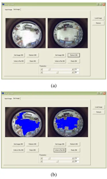
In Step 2.4, the points Bi which belong to Ti and belong to the region of the ground are found, and in Step 3, these points are regarded as seeds and Step 2 is repeated again to check if these points belong to the region or not. No matter whether the point Ti belongs to the region or not, the point will be marked as scanned. An example is shown in Figure 4.2. The two images in Figure 4.2(a) are taken by two

(51)

regions found by the above algorithm.

(a)

(b)

Figure 4.2 An example of finding the region of the ground.

4.2.2 Using Image Coordinates of Ground

Region to Construct a Rough

Environment Map

(52)

can utilize the coordinates to construct a rough environment map by the following method.

Because the mapping tables of the fisheye cameras are constructed in advance, coordinates can be converted between the ICS (image coordinate system) and the GCS (global coordinate system) freely by Algorithm 3.1. And the size of an environment map is defined in advance, so we can convert the global coordinates Gi of each point in the map into image coordinates Ii first.

Also, because all the image coordinates of the ground region Rg have been found

by Algorithm 4.1 in Section 4.2.1, we can check them to see if the image coordinates

Ii specify a point pi belonging to Rg or not. If pi belongs to Rg, then we indicate the

space point Pi of the global coordinates Gi in the map to be an open way otherwise, to be an obstacle. Hence we can obtain the global coordinates of all the obstacles in the environment, and so can indicate the positions of the obstacles in the map to construct a rough environment map.

4.2.3 Eliminating Broken Areas in a Rough

Environment Map

After constructing a rough environment map, there will be a lot of broken areas in the map, so a refining process is applied to eliminate these broken areas. The refining process includes two major operations erosion and dilation. An erosion operation can eliminate the noise in the map, and a dilation operation can mend unconnected areas to make the map smooth.

(53)

of an element E is true, that means there are some obstacles in this region R. A mask with nn size will then be put on R and every element in this mask will be examined

to see if the values of them are true or false. The values of elements in the mask then are gathered to decide the new value of E. If the number of the value of true is larger than half of the number of elements in the mask, then the new value of E will be set

true; otherwise, the value of E will be set false. In another situation, if the value of E

is false originally, the new value of E will be false, too. Because of the property of this erosion operation, the noise in the map will be eliminated.

The dilation operation can expand the region of every obstacle, so if there is a little gap between two regions of obstacles, after doing the dilation operation, the gap will be mended. The dilation operation also scans all of the elements in the map, and if the value of element R is true, another mask with size mm is put on R. Afterward,

the value of every element which is in the mask are set to true, hence every obstacle in the map will be expanded, and the gap will be mended. The degree of expansion depends on the size of mask, that is, if m is large, then the degree of expansion will be high. An example of results is shown in Figure 4.3.

(a) (b)

Figure 4.3 An example of refining a map. (a) A rough map. (b) A complete map after applying the erosion and dilation operations.

(54)

4.3 Avoiding Static Obstacles

After constructing the complete environment map, we can know exactly the positions of the obstacles in an indoor environment. When an autonomous vehicle navigates in the environment, it should avoid all of the obstacles automatically. When there are some obstacles on the original path from a starting point to a terminal point, the system should plan a new path to avoid the obstacles, and the new path will satisfies the following constraints:

1. The shortest path should be chosen.

2. The turning points should be within the open space where no obstacle exists.

3. The number of turning points should be reduced to the minimum.

The method we use in this study is to find several turning points to insert between the original starting point and the terminal point. Here, by a turning point, we mean one where the autonomous vehicle will turn its direction. The lines connecting these points will be the new path. As shown in Figure 4.4, the purple points are the original starting and terminal points, and the red line is the original path.

Figure 4.4 Illustration of computing turning points to construct a new path (composed by blue line segment) different from original straight path (red line

以天花板上多環場攝影機輔助自動車作室內安全監控之研究

國

立

交

通

大

學

多媒體工程研究所

碩

士

論

文

以天花板上多環場攝影機輔助自動車

作室內安全監控之研究

A Study on Indoor Security Surveillance by

Vision-based Autonomous Vehicle With

Omni-cameras on House Ceiling

研 究 生：王建元

指導教授：蔡文祥 教授

以天花板上多環場攝影機輔助自動車

作室內安全監控之研究

A Study on Indoor Security Surveillance by

Vision-based Autonomous Vehicle With

Omni-cameras on House Ceiling

研 究 生：王建元 Student：Jian-Yuan Wang

指導教授：蔡文祥 Advisor：Prof. Wen-Hsiang Tsai

國 立 交 通 大 學

多 媒 體 工 程 研 究 所

碩 士 論 文

以天花板上多環場攝影機輔助自動車

作室內安全監控之研究

研究生：王建元 指導教授：蔡文祥 教授

國立交通大學多媒體工程研究所

摘要

A Study on Indoor Security Surveillance by Vision-based

Autonomous Vehicles with Omni-cameras on House Ceilings

ABSTRACT

ACKNOWLEDGEMENTS

CONTENTS

LIST OF FIGURES

LIST OF TABLES

Chapter 1

Introduction

1.1 Motivation of Study

1.2 Survey on Related Studies

1.3 Overview of Proposed System

1.4 Contributions

1.5 Thesis Organization

Chapter 2

System Configuration

2.1

Introduction

2.2

Hardware

2.3 System Process

Chapter 3

Adaptive Space Mapping Method for

Object Location Estimation Subject

to Camera Height Changes

3.1 Ideas of Proposed Adaptive Space

Mapping Method

3.2 Construction of Mapping Table

3.2.1 Proposed Method for Constructing A

Basic Mapping Table

3.2.2

Using a Point-correspondence

Technique Integrated With An Image

Interpolation Method to Locate

Objects

3.2.3 Proposed Method for Constructing An

Adaptive Mapping Table

3.3 Using Multi-cameras to Expand the

Range of Surveillance

3.3.1 Calculating Relative Position of

Cameras

3.3.2 Calculating Relative

Rotation Angle of

Two Cameras



3.3.3 Calculating Coordinates in The GCS

研究生：王建元

指導教授：蔡文祥教授

研究生：王建元 Student：Jian-Yuan Wang

國立交通大學

多媒體工程研究所

碩士論文

研究生：王建元指導教授：蔡文祥教授