以序的最佳化理論為基礎的多重使用者正交分頻多工系統的適應性次載波指定與位元分配方法

國 立 交 通 大 學

電機與控制工程學系

博 士 論 文

以序的最佳化理論為基礎的多重使用者正交分頻多工

系統的適應性次載波指定與位元分配方法

Adaptive Subcarrier Assignment and Bit Allocation

Methods for Multiuser OFDM System Using Ordinal

Optimization Approach

研 究 生：黃榮壽

指導教授：林心宇 教授

以序的最佳化理論為基礎的多重使用者正交分頻多工系統的適應性次載波指

定與位元分配方法

Adaptive Subcarrier Assignment and Bit Allocation Methods for Multiuser OFDM

System Using Ordinal Optimization Approach

研 究 生： 黃 榮 壽 Student: Jung-Shou Huang

指導教授： 林 心 宇 Advisor: Shin-Yeu Lin

國 立 交 通 大 學

電機與控制工程學系

博 士 論 文

A Dissertation

Submitted to Department of Electrical and Control Engineering College of Electrical Engineering

National Chiao Tung University in partial Fulfillment of the Requirements

for the Degree of Doctor of Philosophy

in

Electrical and Control Engineering October 2008

Hsinchu, Taiwan, Republic of China

以序的最佳化理論為基礎的多重使用者正交分頻多工系統的適應

性次載波指定與位元分配方法

研究生：黃榮壽 指導教授：林心宇 博士

國立交通大學電機與控制工程學系

摘要

下一世代的無線通信系統被期望能夠在無須考慮使用者移動情況與使用者所在位置 的情況下，提供高的資料傳輸率的能力，以符合提供數位影音廣播與無線網際網路等資料 存取服務的需求。要達到此目的會面臨的主要挑戰有幾項: (1)惡劣的無線通道環境，(2) 服務品質，例如資料錯誤率與使用者的資料需求量，(3)通信系統中資源的配置，例如功 率消耗與頻帶資源的管理問題，(4)因為使用者的可移動特性所造成的通信系統狀態變 化。最近，正交分頻多工系統受到熱切的關注且被認為適合被用於下一世代無線通信系統 之中，因為它能夠有效率地傳輸資料，同時能夠抵抗各種傳播通道破壞並克服符間干擾問 題。這個需求趨使我們去發展聰明且有效的資源管理方法，使得在滿足多重使用者的服務 品質需求下，能夠即時的調配整個無線通信系統的功率與頻譜配置，以達到通信系統整體 最有效率的運用。因此在本論文中，我們將提出兩個以序的最佳化理論為基礎的多重使用 者正交分頻多工系統的適應性次載波指定與位元分配方法。 第一個方法採用序的最佳化理論為基礎的四層次演算法來求解一個足夠好的解。在 前三個層次中，我們採用較粗略的模型來從候選的解空間中篩選出一些近似足夠好的可 行解，直到選出 l (=3)個足夠好的解為止。之後的第四個層次中，採用精確的模型來從 這l 個足夠好的解之中篩選出最佳的那一個當做我們所要尋找的足夠好的解。這個四層 次演算法保證能夠獲得一個足夠好的解，但是其中的第一層次耗費很多的計算時間於求 解連續性問題的最佳解，因此我們提出可以採用硬體電路為輔助的方法與架構，利用深 次微米的技術優勢來快速計算出連續性問題最佳解。 在大維度多重使用者正交分頻多工系統問題之中，採用硬體電路來實現第一層次時 會有晶片面積太大的問題，因此在我們提出的第二個以序的最佳化理論為基礎的演算法 中，我們採用一個近似目標函數值的計算模型，配合遺傳演算法來從可能的解空間中， 快速地搜尋出I (=200)個足夠好的解。 經由數值模擬以及與其他現行的方法做比較的結果可知，我們所提出的兩個方法在 解的優質性與計算效率上都很成功，除了有效改善通信系統的功率效益之外，其中的一 個方法可藉由硬體電路的輔助來達到即時應用之需求，而第二個方法很適合用於大維度 多重使用者正交分頻多工系統問題之中。

Adaptive Subcarrier Assignment and Bit Allocation Methods for Multiuser OFDM

System Using Ordinal Optimization Approach

Student: Jung-Shou Huang Advisor: Dr. Shin-Yeu Lin

Department of Electrical and Control Engineering

National Chiao-Tung University

Abstract

The next generation wireless communication systems are expected to provide high rate transmission in the applications of digital audio broadcast, digital video broadcast and wireless internet access but regardless to the users’ mobility and location. The major challenges we are confronted with include the harsh channel conditions, QoS (Quality of Services) requirements such as BER (Bit Error Rate) and users’ data rate request, scarce resources such as power and spectrum, and the knowledge of the most updated state of the mobile users or devices. Orthogonal frequency-division multiplexing (OFDM) technology is recently recognized as one of the leading candidates for supporting the next generation wireless communication systems due to its ability to combat inter-symbol-interference (ISI) over harsh channel conditions. This stimulates the development of both intelligent and efficient resource management algorithms to achieve efficient utilization of power and spectrum while providing QoS requirements in the multiuser OFDM communication system. Therefore in this dissertation, we will present two computationally efficient methods to solve the Adaptive Subcarrier Assignment and Bit Allocation (ASABA) problem of multiuser OFDM system using Ordinal Optimization (OO) approach.

Our first method consists of four OO stages to find a good enough solution to the ASABA problem. In the first three stages, we use surrogate models to select a subset of estimated good

enough feasible solutions from the candidate solution set so as to reduce the search space of

subcarrier assignment until l (=3) good enough subcarrier assignment patterns are obtained. Then in the fourth stage, we use the exact objective function to evaluate the l subcarrier assignment patterns, and the best one associated with the corresponding optimal bit allocation is the good enough solution that we seek. The four-stage OO approach ensures the quality of the obtained solution, however at the cost of solving a continuous version of the considered problem in the first stage. To resolve this computational complexity problem, we propose a hardware implementable Dual Projected Gradient (DPG) method to exploit deep submicron technology so as to obtain the optimal continuous solutionextremely fast.

Due to the large dimension of the ASABA problem, implementing the first stage in hardware is almost impossible for area concern. Therefore in the first stage of our second method, we develop an approximate objective function to evaluate the performance of a subcarrier assignment pattern and use a genetic algorithm to efficiently search through the huge solution space to find I (=200) good solutions.

Numerical results and comparisons with various existing algorithms are provided to demonstrate the potential of the proposed techniques. It is shown that the proposed resource allocation methods substantially improve the system’s power efficiencies and are more computationally efficient. Moreover, the first method can meet the real-time application requirement and the second method is suitable for large dimensional ASABA problems.

誌 謝

首先要感謝我的指導教授林心宇博士在論文研究上給予的細心指導及

鼓勵，且提供優良的研究環境，使我能順利完成博士學位。林心宇教授學

問淵博、涵養深厚，在學術研究上見解精闢、邏輯縝密，研究認真精神與

嚴謹程度實在值得效法。對於本論文的完成，除了林教授的指導外，也要

非常感謝諸位口試委員在百忙之中能抽空指導並給予寶貴的意見，使得本

論文能更臻完善。

其次，要感謝我的學長林啟新博士、林謝興博士與洪士程博士，實驗

室的學弟張紹興、林成梓與詹庭瑜。多年來，因為有你們的參與，使我在

交通大學的求學過程之中，添增了一些多采多姿的回憶。

同時也要感謝我的服務單位，義隆電子公司的長官與同事們多年來的

協助，使我得以順利完成此論文。

最後，感謝作者的父母與妻兒，在求學期間的支持與陪伴，讓我可以

全心全力的專注於論文研究上。僅以此論文獻給我的家人與關心我的師長

與朋友們。

Contents

Abstract (Chinese) i

Abstract (English) ii

Acknowledgement (Chinese) iii

Contents iv

List of Tables vi

List of Figures vii

1 Introduction ……….1

1.1 Motivation ……….1

1.2 Problem Statement ……….2

1.3 Dissertation Outline………..………..2

2 Preliminaries ……….5

2.1 Multiuser Orthogonal Frequency Division Multiplexing System ……..……..5

2.2 Adaptive Subcarrier Assignment and Bit Allocation (ASABA) Problem …....6

2.3 Review of Ordinal Optimization Theory ………..……..……..………..……..9

2.4 Review of Genetic Algorithm .……..……..…..………..……..………..10

2.5 Review of Artificial Neural Network …..…..……..……..……..……..……..11

3 A Real-Time Method for Adaptive Subcarrier Assignment and Bit Allocation problem of Multiuser OFDM System .……….……….13

3.1 The Dual Projected Gradient Method and Its Hardware Architecture ……....14

3.1.1 Reformulation …..……..……..……..…..……..……..……..……..….14

3.1.2 The Dual Projected Gradient (DPG) Method for Solving (3.2) …...15

3.1.3 Hardware Implementable Algorithm of the DPG Method …...17

3.1.4 Hardware Computing Architecture of the DPG Algorithm …...19

3.1.5 Computation Complexity of the DPG Algorithm ……….…...26

3.2 The Ordinal Optimization Theory Based Four-Stage Approach ……...27

3.2.1 Stage 1: Reduce the Search Space of Subcarrier Assignment Using Continuous Optimal Solution Based Model ……..….……..……..….27

3.2.2 Stage 2: Choose s Estimated Good Enough Subcarrier Assignment Patterns Using an Approximate Model .….……..……..…..……....….29

3.2.3 Stage 3: Choose l Estimated Good Enough Subcarrier Assignment Patterns from the SS ……..……..…..……..……..……..……..……....30

3.2.4 Stage 4: Determine the Good Enough Subcarrier Assignment

and Bit Allocation ……..……..…..……..……..……..…….…...….32

3.3 Test Results and Comparisons ……..……..…..……..……..……..…...….32

3.4 Concluding Remarks……..……..…..……..……..……..……….…….38

4 A Computationally Efficient Method for Large Dimension Subcarrier Assignment and Bit Allocation Problem of Multiuser OFDM System …….….39

4.1 Reformulation ..……..…..……..……..…….. ………..…….41

4.2. The Three-Stage Ordinal Optimization (OO) Approach ……….…….43

4.2.1 Stage 1: Using GA to Select Top s Subcarrier Assignment Patterns Based on an Easy-to-Evaluate Approximate Objective Function ..….43

4.2.2 Stage 2: Choose Top l Subcarrier Assignment Patterns From the s Based on an ANN Model .……..…..……..……..……….….….46

4.2.3 Stage 3: Determine the Good Enough Subcarrier Assignment and Bit Allocation .……..…..……..…………..………..…….48

4.3 Test Results and Comparisons …..………...…………..………..…….48

4.4 Concluding Remarks…..……..…………..………...……53

5 Conclusions and Future Work ……….………55

5.1 Conclusions…..……..…………..…………...………...……55

5.2 Future Work…..……..…………..……….………....……56

References…..……..………..……….…...……57

List of Publication…..……..………..……….…..……61

List of Tables

Table 3.1 The characteristics of PEs …..……..…………..………..……22 Table 3.2 Average computation time (ms) for obtaining an abSNR(αi) for

various number of users. …..……..…………..………..……36 Table 3.3 The average − ×100%

d D d

List of Figures

Figure 2.1 Block diagram of a multiuser OFDM system with subcarrier

assignment and bit allocation. ………...5 Figure 2.2 An example of channel gain. ………..………...7 Figure 2.3 The GA procedure to the proposed ………..10 Figure 2.4 Diagram of a simple feed-forward ANN with a single hidden layer. ..11 Figure 3.1 The three types of registers for storing the temporary computed

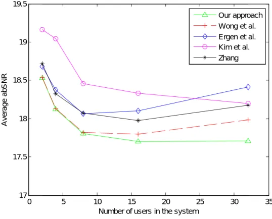
values of the DPG algorithm.………..………..20 Figure 3.2 The three counters.………..………..23 Figure 3.3 The hardware architecture of the DPG algorithm.…..………..25 Figure 3.4 The abSNR for K=2, 4, 8, 16, and 32 obtained by the five methods....34

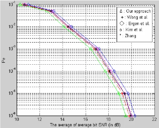
Figure 3.5 Comparison of the performance of the five methods with respect to variousPe for the case of K=7.………..………...35

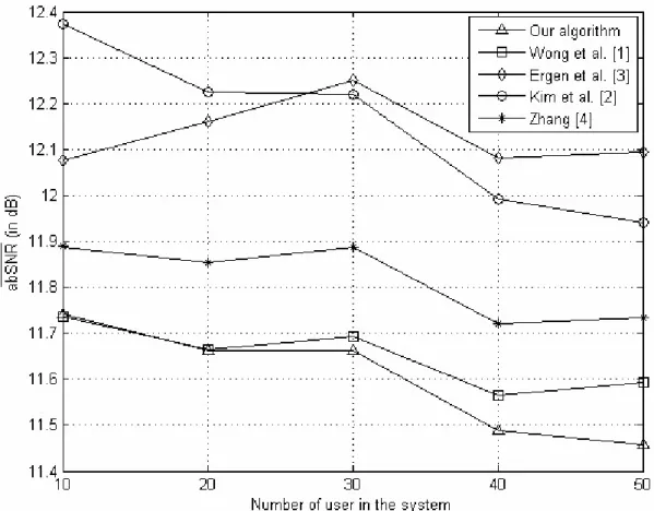
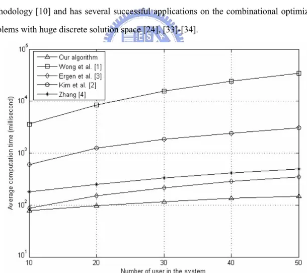
Figure 4.1 The abSNR for K=10, 20, 30, 40 and 50 obtained by the five

algorithms.………..………..………...50 Figure 4.2 The average computation time for obtaining an abSNR by the five

algorithms in cases of K=10, 20, 30, 40 and 50.………..…………...51 Figure 4.3 Comparison of the five algorithms for various Pe in the case of

Chapter 1

Introduction

1.1 Motivation

Due to the increase of mobile users and devices in the wireless communication system, various resource management techniques such as the dynamic channel allocation [1] and the dynamic fair resource allocation scheme [2] had been studied. One of the difficulties for such kind of techniques is to keep track of the most updated state of the mobile users or devices caused by their mobility and portability and provide them the appropriate resources. Therefore, the computational efficiency is the premise of the wireless network resource management methods so as to deal with the high mobility of the dynamic behaviors of mobile users and devices. Among the existing dynamic resource management problem in wireless networks, Adaptive Subcarrier Assignment and Bit Allocation (ASABA) of Orthogonal Frequency Division Multiplexing (OFDM) system is a very fundamental issue in mobile communication. There are two types of formulations on this issue. One is the Margin Adaptive (MA) optimization, which minimizes the total consumed power under a data rate constraint [3], and the other is the Rate Adaptive (RA) optimization, which maximizes the data rate under a power constraint [4]. Kim et al. had shown in [5] that the RA optimization problem can be solved via recursive MA optimization. Therefore, in this dissertation we will focus on the adaptive subcarrier assignment and bit allocation problem of MA optimization with emphasis on the solution quality and the computational efficiency.

In general, to obtain a better solution of a hard optimization problem such as the resource management problem in the wireless communication system usually requires a sophisticated but computationally intensive algorithm. In this dissertation, we will revolt this seemingly correct argument by proposing two methods that will not only obtain a good enough feasible

solution but also be computationally efficient. The first method can meet the real-time

application requirement while with the assistance of hardware. The second method is purely a software but still computationally efficient for solving the large dimension ASABA problem of multiuser OFDM system.

1.2 Problem Statement

The adaptive subcarrier assignment and bit allocation of multiuser OFDM system has been studied for a number of years. This issue is initialized by Wong et al. in [3] and is formulated as a nonlinear integer programming problem to minimize the total power consumption while satisfying the users’ data communication request and system’s constraints. Wong et al. employed a Lagrangian relaxation method in [3] to solve the continuous version of the adaptive subcarrier assignment and bit allocation problem. They then rounded the optimal continuous subcarrier assignment solution off to the closest integer solution. Although the algorithm dramatically enhances the power efficiency, the prohibitively high computational complexity renders it impractical. Since then, various methods, ranging from the more computation-time consuming and global-like mathematical programming based approach [5] to the less computation-time consuming and more local-like schemes [6]-[9] were proposed to cope with this NP-hard constrained combinatorial optimization problem. In [5], Kim et al.

had converted the adaptive subcarrier assignment and bit allocation problem formulated in [3]

into a linear integer programming problem and employed a suboptimal approach to separately

perform the subcarrier assignment and bit allocation. To claim for computational efficiency by

not using mathematical programming approach, Ergen et al. had proposed in [6] a heuristic

two-module scheme, both Kivanc et al. and Zhang had proposed two-step subcarrier

assignment approaches in [7] and [8], respectively, and Han et al. had proposed in [9] an iterative grouping scheme to improve the performance by exchanging subcarrier assignment sets. As a consequence, these approaches cannot yield a better solution while using limited computation time due to the nature of nonlinear optimization.

1.3 Dissertation Outline

The dissertation introduces two computationally efficient methods to solve the ASABA problem of multiuser OFDM system using Ordinal Optimization (OO) approach. Since both methods are multi-stage OO based approaches, there are some overlap. For the sake of completeness in presenting each individual method, the overlapping part will be duplicated. Therefore, we organize this dissertation in the following manner.

These include OFDM architecture based communication system, adaptive subcarrier assignment and bit allocation for multiuser OFDM, OO theory, Artificial Neural Network (ANN), and Genetic Algorithm (GA). The OFDM is a promising technology for high data rate transmission in wide band wireless systems due to its ability to mitigate the effects of frequency selective and combat Inter-Symbol Interference (ISI). The adaptive subcarrier assignment and bit allocation for multiuser OFDM communication system can be formulated as a nonlinear integer programming problem to minimize the total power consumption while satisfying the users’ data communication request and system’s constraints. The OO theory is a new methodology designed to cope with hard optimization problems such as the considered problem. The GA acts as a heuristic method to select a representative set for the search space of the considered problem. The ANN is trained as an easily computed crude model to roughly evaluate the performance of the considered problem.

In chapter 3, we present an OO theory based four-stage approach to deal with the subcarrier assignment and bit allocation problem of multiuser OFDM system. The four-stage OO approach ensures the quality of the obtained solution, however at the cost of solving a continuous version of the considered problem in the first stage. To resolve this computational complexity problem, we propose a hardware implementable Dual Projected Gradient (DPG) method to exploit deep submicron technology. Therefore, our approach can meet the real-time application requirement through the assistance of hardware.

In chapter 4, we present another OO theory based three-stage approach to deal with the

large-dimension ASABA problem of multiuser OFDM system. First of all, we reformulate the

considered problem to separate it into subcarrier assignment and bit allocation problem such that the objective function of a feasible subcarrier assignment pattern is the corresponding optimal bit allocation for minimizing the total consumed power. Then in the first stage, we develop an approximate objective function to evaluate the performance of a subcarrier assignment pattern and use a genetic algorithm to search through the huge solution space and select s best subcarrier assignment patterns based on the approximate objective values. In the second stage, we employ an off-line trained ANN to estimate the objective values of the s subcarrier assignment patterns obtained in stage 1 and select the l best patterns. In the third

stage, we use the exact objective function to evaluate the l subcarrier assignment patterns obtained in stage 2, and the best one associated with the corresponding optimal bit allocation is the good enough solution that we seek.

Some conclusions for the dissertation are drawn in Chapter 5. We also suggest some possible future research issues concerning the methods developed in this dissertation.

Chapter 2

Preliminaries

2.1 Multiuser Orthogonal Frequency Division Multiplexing System

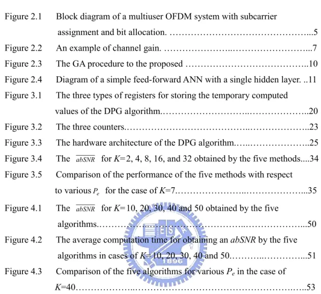
The basic idea of OFDM is to divide the available spectrum into several subcarriers so that the information symbols are transmitted in parallel on the subcarriers over the wireless channel. This allows us to design a system as shown in Figure 2.1 to support high data rates transmission.

We assume that the system has K users to share N subcarriers. Each user’s data rate request will be allocated to a nonoverlapping set of subcarriers and distributed among them. The allocating period in this model is a time interval consisting of several OFDM symbols and is assumed to be short enough so that users’ channel gains will stay approximately constant. It is also assumed that a subcarrier cannot be shared by more than one user.

In the transmitter part of Figure 2.1, the serial data from K users are fed into the block represented by the proposed adaptive subcarrier assignment and bit allocation algorithm. The algorithm will be executed in every allocating period to assign the set of subcarriers to each

Subcarrier assignment and bit allocation Data of user 1 Data of user 2 Data of user K . . . . . . . . Adaptive modulator 1 IFFT Add Guard Interval

Base station transmitter

Remove Guard Interval User k receiver Data of user k Channel information from K users

Figure 2.1. Block diagram of a multiuser OFDM system with subcarrier assignment and bit allocation.

Adaptive modulator 2

Adaptive modulator N

Frequency Selective Fading Channel for

the thk user FFT . . . . Adaptive demodulator 1 Adaptive demodulator 2 Adaptive demodulator N Extract bits for the th k user The resource allocation module

user and the number of bits to be transmitted on each assigned subcarrier based on the updated channel information of all users. For each subcarrier, the adaptive modulator will apply a proper modulation scheme to each symbol depending on the number of bits assigned to the subcarrier, and the modulated symbols are transformed into time domain samples by an Inverse Fast Fourier Transform (IFFT) as indicated in Figure 2.1. The guard interval is then added to ensure orthogonality between the subcarriers provided that the maximum time dispersion is less than the guard interval. Finally, the transmitted signals pass through different frequency selective fading channels to different users.

We assume the subcarrier assignment and bit allocation information is sent to the receivers via a separate control channel. For the sake of simplicity, we only show the receiver part of one user in Figure 2.1. At the kth user’s receiver part, the guard interval is removed to

eliminate the ISI, and the time sample of the kth user is transformed into modulated symbols

using the Fast Fourier Transform (FFT). The modulation information is then used to configure the demodulators while the subcarrier assignment information is used to extract the

demodulated bits from the subcarriers assigned to the kth user.

2.2 Adaptive Subcarrier Assignment and Bit Allocation (ASABA) Problem

In OFDM communication system, the power level needed for transmitting c bits from transmitter to user k receiver using subcarrier n is ₂

, ) ( n k k c f

α , where fk(c) denotes the required

transmission power for c bits of user k when the channel gain is equal to unity and αk ,n

denotes the magnitude of the channel gain of the nth subcarrier as seen by the kth user. Just as an example, we assume that M-ary QAM is used in the communication system, then the required power f_k(c) in ₂ , ) ( n k k c f

α to transmit c bits/symbol can be derived from [3] 1_: )] (2 1) 4 ( [ 3 ) ( = 0 −1 e 2 c− k P Q N c f (2.1)

where Q−1(x) is the inverse function of

1 _{The formula (2.1) is directly borrowed from [3, Sec. V, p.1725], which is an approximation based on the}

bit-error probability, 4Q( d2/(2N₀)), and the average energy, (M−1)d2/6, of a MQAM symbol, where d is the minimum distance between the points in the signal constellation.

Q x e dt x t

∫

∞ − = 2 2 2 1 ) ( π (2.2),

N0 denotes the noise Power Spectral Density (PSD) level, and Pe denotes the BER.

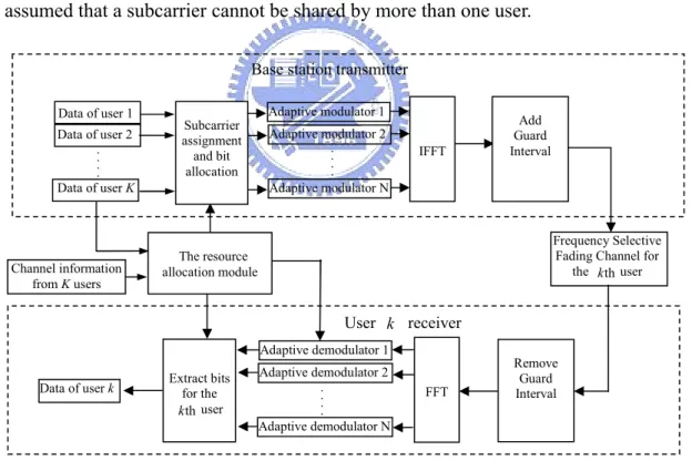
In general, wireless link capacity is generally a scarce resource that needs to be used efficiently. The channel-gain conditions of wireless links between transmitter and mobile users vary in the time domain, and different subcarriers experience different channel gains. Therefore,the subcarriers which appear in deep fade to one user may not be in deep fade for other users. A typical example of channel gains, α_{k ,n}’s, in ₂

, ) ( n k k c f

α can be shown in Figure 2.2,

and a lower magnitude of the channel gain represents a deeper fade channel condition.

Figure 2.2. An example of channel gain.

Therefore, multiuser OFDM communication system can take the advantage of channel diversity among users in different locations to adaptively assign subcarriers and allocate modulation levels. In particular, large subcarrier gains result in higher order modulation to carry more bits/symbol, while subcarriers in deep fade carry one or even zero bits/symbol.

Hence power consumption can be greatly reduced under a good resource allocation scheme. Then, the adaptive subcarrier assignment and bit allocation for multiuser OFDM system can be formulated as a nonlinear integer programming problem as shown in (2.3) to minimize the total power consumption while satisfying the users’ data communication request and system’s constraints2.In this dissertation, we focus on proposing an efficient and effective algorithm to solve (2.3) for a good enough feasible solution.

) ) ( ( min 1 1 , 2 , , , _, ,

∑∑

_{= =} = N n K k n k k n k n k T c_{kn kn}P α f c ρ ρ subject to R N c k K n n k k , 1,..., 1 , = =

∑

= N n K k n k 1, 1,..., 1 , = =

∑

= ρ k,n D c_k,n∈ ,for all ck,n k,n n

k _{1 otherwise}, for all

0 if 0 , ⎩ ⎨ ⎧ = = ρ (2.3)

where P denotes the total transmission power to be minimized; _T ρ is an indicator _{k ,n}

variable, and a subcarrier can be occupied by at most one user as described by the equality constraint on ρ ; _{k ,n} R (bits per OFDM symbol) denotes the requested data rate of the _k

th

k user; c_k,n denotes the number of bits of the kth user assigned to the nthsubcarrier, and M} 2,..., , 1 , 0 { =

D denotes the set of all possible values for c_k,n, thus the first equality constraint in the problem formulated in (2.3) implies that the subcarrier assignment and bit allocation should meet the user’s data rate request.

Clearly, (2.3) is a nonlinear integer programming problem or a constrained combinatorial optimization problem, because ρk,n and ck,n are integers for all k, n, and PT is nonlinear. To

cope with the computational complexity of this problem, we will employ the OO theory based algorithms to efficiently seek a good enough solution with high probability instead of searching the optimal solution.

2.3 Review of Ordinal Optimization Theory

The Ordinal Optimization theory [10]-[12] is a new methodology designed to deal with hard problems such as the lack of structure problems, problems with uncertainties, or problems with huge sample space that grows exponentially with respect to the problem size. The problem considered in this dissertation is of the latter kind. There are two basic tenets of the OO theory. The first is that of order versus value in decision making. Obviously, to determine whether PT(ρ1,c1)<PT(ρ2,c2) is much easier than to determine

? ) , ( ) , ( 2 c2 −P 1 c1 =

P_T ρ _T ρ . In other words, consider the intuitive example of determining which

of the two boxes in two hands is heavier versus identifying how much heavier one is than the other. The second tenet is the goal softening. Instead of asking the best for sure in optimization, it settles for the good enough with high probability. A conclusion drawn from the OO theory is the following.

Suppose we simultaneously evaluate a large set of alternatives very approximately and order them according to the approximate evaluation. Then there is high probability that we can find the actual good alternatives if we limit ourselves to the top n% of the observed good choices.

Firstly, we use only a very rough model to order the goodness of a solution relying on the robustness of ORDER against noise and model error to separate the good from the bad. Second, we soften the goal of the problem and look for a good enough solution, which is among the top n% of the search space, with high probability. These two steps greatly reduce the computational burden and search difficulties of the problem. A summary of these search procedures for obtaining a good enough feasible solution of ASABA problem with high probability can be described in the following: i) Using either a uniform selection or a heuristic method to select a feasible representative set I with size I for the search space. ii) Using an easily computed crude model to roughly evaluate and order the performance of each sample in I and collect the top s samples to form a selected subset (SS), which is the estimated good enough subset. The OO theory guarantees that SS consists of actual good enough solutions with high probability. iii) Evaluating the exact objective value for each sample in SS to obtain the good enough solution.

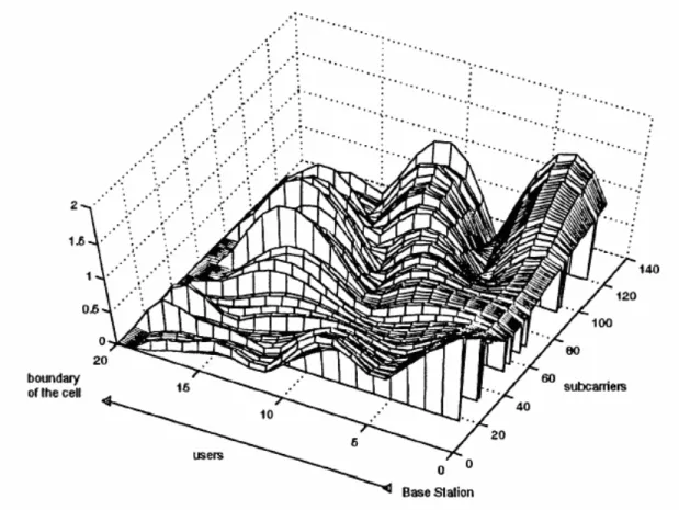
2.4 Review of Genetic algorithm

Genetic algorithm [13]-[16] is population-based searching technique based on the idea of “survival of the fittest”, which repeats evaluation, selection, crossover, mutation and repair after initialization until a stopping criterion is satisfied. In a GA, a set of solutions are analyzed and modified by genetic operations simultaneously, where selection operator can select some “good” solutions as seeds, crossover operator can generate new solutions hopefully retaining good features from parents, mutation operator can enhance diversity and provide a chance to escape from local optima, and repair operator can avoid infeasible solutions during the evolving processes.

In this dissertation, GA is used in the second method to select I good solutions from the search space of the considered problem. The flow chart of the GA used in our approach is shown in Figure 2.3.

Generate an initial generation Set g=0

Start

Calculate estimated objective value using crude

model for each population in the generation

Crossover Roulette wheel selection Mutation pc pm Repair g=g+1 if g<60

Output the evolved generation as the representative set

Figure 2.3. The GA procedure to the proposed method.

2.5 Review of Artificial Neural Network

An Artificial Neural Network [17]-[19] is a mathematical model or computational model based on biological neural networks, which learns from previously prepared input/output data then to determine the output data for a given input data. The key element of ANN is the novel structure of the information processing system. It is composed of a large number of highly interconnected processing elements (neurons) working in unison to solve specific problems. Through a learning process, various types of ANN models can be effectively used for many applications, such as pattern recognition, function approximation or data classification. In this dissertation, a simple feed-forward ANN is employed as a crude model to roughly evaluate the objective value of the considered problem, (2.3).

Figure 2.4. Diagram of a simple feed-forward ANN with a single hidden layer.

A diagram of a simple feed-forward ANN with a single hidden layer is shown in Figure 2.4. The ANN consists of one input layer, one hidden layer, and one output layer. Each layer contains neurons (circles in the figure), and the neurons in each layer are fully connected to the nearest layers above or below by the lines. A weight is associated with each arc line. The neurons in the input layer receive the input vectors, and neurons in the output layer produce the output vectors in response to the input vectors. The layers are connected through the weighted arcs. Neurons in hidden layers and the output layer perform two operations: they sum the products of arc weights and the signals from the previous layer, and pass that sum through a transfer function—often a sigmoid, hyperbolic

∑

_f

∑

_f

∑

_f

∑

_f

∑

_f

∑

_f

Input #1 Input #2 Input #3 Input #4 Output

tangent sigmoid, or linear function.

Supervised learning can be used to train an appropriately configured ANN to implement a mapping. In our methods, an ANN is off-line trained and is employed as a surrogate model to estimate the objective value of the considered problem.

Chapter 3

A Real-Time Method for Adaptive Subcarrier Assignment and Bit

Allocation problem of Multiuser OFDM System

To deal with the high mobility of the dynamic behaviors of mobile users and devices, the real-time application requirement is the premise of the wireless network resource management solution methods. Therefore, in this chapter we will present an OO theory based four-stage approach for the subcarrier assignment and bit allocation problem of multiuser OFDM system with emphasis on the solution quality and the computational efficiency to meet the real-time application requirement.

In the first three stages, we will use surrogate models to select a subset of estimated good

enough feasible solutions from the candidate solution set so as to reduce the search space of

subcarrier assignment until l (=3) good enough subcarrier assignment patterns are obtained. The surrogate models in these three stages are refined from stage to stage, because the required computation time has become less as the size of the candidate solution set diminishes. Then in the fourth stage, we will employ a greedy algorithm [20] for single user on each of the

l subcarrier assignment patterns to obtain the corresponding optimal bit allocation, and the one

achieving the smallest power consumption will be the good enough feasible solution that we seek. The most computationally intensive stage among the four lies in the first stage, in which we need to solve a continuous version of the considered problem. To cope with the computational complexity caused by the nonlinear programming algorithm, we propose a

hardware implementable numerical method to exploit the merit of nowadays integrated circuit technology so as to obtain the optimal continuous solutionextremely fast. Therefore, our OO theory based four-stage approach not only obtains a good enough feasible solution but also meets the real-time application requirement.

We organize chapter 3 in the following manner. In Section 3.1, we will present the Dual Projected Gradient (DPG) method to solve the continuous version of the considered problem. In the meantime, we will also present the hardware architecture of the DPG method. In

Section 3.2, we will present the OO theory based four-stage approach for finding a good enough feasible solution. In Section 3.3, we will present some test results and compare our approach with some existing methods in the aspects of power consumption and computation time. In Section 3.4, we will make a conclusion.

3.1 The Dual Projected Gradient Method and Its Hardware Architecture

3.1.1 Reformulation

Since problem (2.3) is a computationally intractable combinatorial problem, Wong et al. introduced the variable rk,n =ck,nρk,n to transform (2.3) into the following

continuous-variable convex optimization problem over a convex set. ) ( min , , 1 1 2, , ] 1 , 0 [0, ] [ , , , n k n k k N n K k kn n k M r r f n k n k n k α ρ ρ ρ ρ

∑∑

= = ∈ ∈ subject to R N r k K n kn k , 1,..., 1 , = =

∑

= K n N k n k , 1,..., 1 1 , = =

∑

= ρ (3.1) where both ρk,n and rk,n are continuous variables, satisfying 0≤ ρk,n ≤1 , and

n k n

k M

r_{, ,}

0≤ ≤ ρ , respectively. Note: when ρk_,n =0, then rk,n =0, and ₀0 becomes undefined,

therefore, we define ) 0 0 (

f in (3.1) as f(0).

If we apply a typical Lagrangian relaxation method to solve (3.1), there will be a singularity problem in the variable ρ just like that shown in [3]. In order to develop a hardware _{k ,n} implementable dual-type method, we need to eliminate this singularity problem by adding extra terms in the objective function of (3.1) to strictly convexifyρ , for every _{k ,n} k,n, as follows:

∑∑

∑∑

= = = = ∈ ∈ + N n K k n k n k n k k N n K k kn n k M r r f n k n k n k _{1 1} 2 , , , 1 1 2, , ] 1 , 0 [, ] 0 [ ( ) 2 min , , , ρ σ ρ α ρ ρ ρ

subject to R N r k K n n k k , 1,..., 1 , = =

∑

= K n N k kn ,..., 1 , 1 1 , = =

∑

= ρ (3.2) If σ >0, (3.2) is a convex programming problem with strictly convex objective function.

Remark 3.1: (i) Adding the extra terms

∑∑

= = N n K k n k 1 1 2 , 2 ρ

σ _{will help us build the surrogate model}

in Stage 1 of our OO theory based four-stage approach as will be shown later. (ii) The optimal solution of (3.2) is a good approximate solution of (3.1) provided that σ is small enough. 3.1.2 The Dual Projected Gradient (DPG) Method for Solving (3.2)

The DPG method will solve the dual problem of (3.2), as shown in (3.3), instead of solving (3.2) directly. max

φ

(

λ

) (3.3) where T N r K r_{,..., , ,..., )} (λ₁ λ λ₁ρ λρ

λ= is the Lagrange multiplier vector such that r k

λ corresponds to the kth user’s data rate request constraint, and λρ_n corresponds to the nth subcarrier assignment constraint, and the dual function φ(λ) is defined by

) 1 ( ) ( 2 ) ( min ) ( 1 , 1 1 , 1 1 1 2 , , , 1 1 2, , ] 1 , 0 [, ] 0 [ , , , − + − + + =

∑∑

∑∑

∑

∑

∑

∑

= = = = = = = = ∈ ∈ K k n k N n n N n n k k K k r k N n K k n k n k n k k N n K k kn n k M r R r r f n k n k n k ρ λ λ ρ σ ρ α ρ λ φ ρ ρ ρ (3.4) By suitably rearranging the terms, (3.4) can be rewritten in a more compact form as

} 1 1 2 ) ( { min ) ( 2_{, , ,} , , 1 1 2, , ] 1 , 0 [, ] 0 [ , , , ρ ρ ρ ρ λ ρ λ λ λ ρ σ ρ α ρ λ φ kn rk k rk kn n kn n n k n k k N n K k kn n k M r N R r K r f n k n k n k − + − + + =

∑∑

= = ∈ ∈ (3.5)

The DPG method employs the following iterations to solve (3.3):

)) ( ( ) ( ) ( ) 1 (t

λ

t

β

t

φ

λ

t

λ

+ = + ∇ (3.6) where t denotes the iteration index, β(t) is a positive step-size and

T N r K r t t t t t)) ( ( ()),..., ( ()), ( ()),..., ( ())) ( ( 1 1 ρ λρ λ φ λ λ φ λ λ φ λ λ φ λ φ ∂ ∂ ∂ ∂ ∂ ∂ ∂ ∂ =

∇ is the gradient of φ( tλ( )) evaluated at

) (t λ

K k r R t N n n k k r k ,..., 1 , ˆ )) ( ( 1 , = − = ∂ ∂

_∑

= λ λ φ _(3.7) N n t K k n k n ,..., 1 , 1 ˆ )) ( ( 1 , − = = ∂ ∂

_∑

= ρ λ λ φ ρ (3.8)

The (_rˆT_,ρˆT)₌(_rˆ_1,1,...,_rˆ_K,N,_ρˆ_1,1,...,_ρˆ_K,N) _{in (3.7) and (3.8) is the solution of the} minimization problem on the RHS of (3.5) for a given λ . Therefore to obtain (t) ∇φ( tλ()), we need to solve for rˆ and ρˆ first, and the key for making the DPG method hardware

implementable is we use a two-phase strategy to fulfill this task.

The first phase is to solve the minimization problem on the RHS of (3.5) without the inequality constraints on r_k,n andρ_{k ,n} , which is shown in (3.9) and will be called the

unconstrained minimization problem.

} 1 1 2 ) ( { min 2_{, , ,} , , 1 1 2, , σ _{ρ λ λ λ}ρ_{ρ λ}ρ ρ α ρ n n k n n k r k k r k n k n k n k k N n K k kn n k K r R N r f + + − + −

∑∑

= = (3.9)

We denote the optimal solution of the unconstrained minimization problem (3.9) by ) ~ ,..., ~ , ~ ,..., ~ ( ) ~ ~

(_rT_,ρT _{= r1,1 rK,N ρ1,1 ρK,N . (}~_rT_,~_ρT_{)can be obtained from solving the first order}

necessary conditions, which can be fully decomposed into N⋅K independent 2x2 equations as shown below: For n=1,...,N,k=1,...,K,

0 ) ( ) ~ ~ ( 1 , , 2 , = − ′ r t f r k n k n k k n k λ ρ α (3.10) 0 ) ( ~ ] ~ ~ ) ~ ~ ( ) ~ ~ ( [ 1 , , , , , , , 2 , = + + ′ − f r r t r f kn n n k n k n k n k k n k n k k n k ρ λ ρ σ ρ ρ ρ α (3.11)

For each n and each k, the simple 2x2 equations shown in (3.10) and (3.11) can be solved analytically by ) ) ( ( ~ ~ 2 , 1 , ,n kn k rk kn k f t r =ρ ′− λ α (3.12) σ α λ α λ α λ α λ ρ ρ_{( )} 1 _{[ ( ( ( ) )) ( ) ( ( ) )]} ~ 2 , 1 2 , 2 , 1 2 , , n k r k k n k r k n k r k k k n k n n k t f t t f f t − ′− − ′− = (3.13)

the f given in (2.1).

The second phase is to handle the inequality constraints disappearing in (3.9) by projecting (~r_k,n,ρ~_k,n) onto the range [0,Mρk_,n]×[0,1], for each k and each n . The projection can be calculated based on simple geometry as shown in (3.14).

⎪ ⎪ ⎪ ⎪ ⎪ ⎪ ⎩ ⎪ ⎪ ⎪ ⎪ ⎪ ⎪ ⎨ ⎧ − < < < > ≤ ≤ > ≤ < ≤ ≤ ≤ ≤ ≤ − + ≤ ≤ − > + + + + − + > > = n k n k n k n k n k n k n k n k n k n k n k n k n k n k n k n k n k n k n k n k n k n k n k n k n k n k n k n k n k n k M r r M r r r M r r M M M r M M r M r M M r M M M M M M r M r M r , , , , , , , , , , , , , , , , , , , , , , , 2 , , 2 , , , , , ~ 1 ~ , 0 ~ if ) 0 , 0 ( 0 ~ , 1 ~ if ) 1 , 0 ( ~ 0 , 1 ~ if ) 1 , ~ ( 0 ~ , 1 ~ 0 if ) ~ , 0 ( ~ ~ 0 , 1 ~ 0 if ) ~ , ~ ( ~ 1 1 ~ ~ 1 , ~ ~ if )) ~ 1 ~ ( 1 ), ~ ~ ( 1 ( ~ 1 1 ~ , ~ if ) 1 , ( ) ˆ , ˆ ( ρ ρ ρ ρ ρ ρρ ρ ρ ρ ρ ρ ρ ρ ρ ρ (3.14)

The resulted projection will be the optimal solution, (_rˆT,_ρˆT)₌ (_rˆ_1,1,...,_rˆ_K,N,_ρˆ_1,1,...,_ρˆ_K,N)_{, of}

the minimization problem on the RHS of (3.5) as had been proven in [22] and [23].

Convergence of the DPG method using a positive constant step-size βˆ (i.e. setting )

(t

β =βˆ for every t) can be proved like that of the Dual Projected Pseudo Quasi Newton method in [22] and [23]. A typical value of βˆ is 0.5.

As indicated previously, the optimal solution of (3.2) will be an approximate solution of (3.1) if σ is sufficiently small. However, larger σ will speed up the convergence of the DPG method. Thus, we let σ₀(=1),σ₁,...,σ_jmax be a decreasing sequence of σ such that

j

j ησ

σ ₊₁= , where η(<1) is a reducing factor, and j_max is a positive integer that makes )

( max max

j j η

σ = small enough. Then, we can initially set σ =σ₀ in (3.2) and use the obtained optimal solution as the initial guess to solve (3.2) again with σ = . Repeating this process σ₁ until σ =σ_jmax , and the corresponding optimal solution of (3.2) will be a very good approximate solution of (3.1).

3.1.3 Hardware Implementable Algorithm of the DPG Method

implement the DPG method. To do so, we need to put the DPG method in algorithmic steps that can be mapped into the operations of the arrays of Processing Elements (PEs), which are defined as the hardware for carrying out the arithmetic operations in the DPG method. First of all, we should modify the convergence criteria of the DPG method by setting a large enough number of iterations, say t_max, such that if t≥t_max, we assume the DPG method converges. Furthermore, we should predetermine the value of j_max , which is the number of times that

σ will be reduced.

It can be observed that all the computation formulae of the DPG method, (3.7), (3.8), (3.12), (3.13), and (3.14), achieve a complete decomposition property, that is the computations for each k and each n can be carried out independently. Furthermore, all these computations consist of simple arithmetic operations only. These facts imply that the DPG method is very suitable for hardware implementation. However, it is not wise to assign a PE to calculate each individual component, for example calculating ρ~_k,n for every k and every n in (3.13), because this will make the size of the integrated circuit chip too big to be implemented. Therefore, to render the difficulty of chip size we can use N arrays of PEs such that the

th

n PE array will take care of all the K computations corresponding to one n in (3.7), (3.8), (3.12)-(3.14). Although such arrangement seems to degrade the computational speed, in fact it will not affect the purpose of real-time application as shown in Section 3.3. On the basis of using N PE arrays, we can put the DPG method in the following parallel-computation algorithmic steps:

Step 0: Set the values of λ(0), σ(0), η (<1), t_max, j_max; set j =0 and t =0.

Step 1: Set k =1, ( ( ( )))=−1 ∂ ∂ ρ λλ φ n t

R for each n . (Note: ( ( _ρ( )))

λ λ φ n t R ∂ ∂ _{represents a}

temporary memory for the term _ρ

λ λ φ n t ∂ ∂ ( ( )) ).

Step 2: Compute in parallel (~rk,n,ρ by calculating (3.12) and (3.13) for each n . ~k,n)

Step 3: Project in parallel (r~k,n,ρ onto the range ~k,n) ([0,Mρk,n],[0,1]) for each n using

Step 4: Compute

∑

= − = ∂ ∂ N n n k k r k r R t 1 , ˆ )) ( ( λ λ φ _.

Step 5: Compute in parallel _kn

n n t R t R( ( ( ))): ( ( ( ))) ρˆ _, λ λ φ λλ φ ρ ρ _∂ + ∂ = ∂ ∂ _{for each n.} Step 6:Update _r k r k r k t t t λ λ φ β λ λ ∂ ∂ + = +1) ( ) ˆ ( ( )) ( .

Step 7: If k=K, go to Step 8; otherwise, set k = k+1 and return to Step 2.

Step 8: Update in parallel ρ ρ _ρ

λ λ φ β λ λ n n n t t t ∂ ∂ + = +1) ( ) ˆ ( ( ))

( for each n . (Note: the value of

∑

= − = ∂ ∂ K k n k n t 1 , 1 ˆ )) ( ( _ρ λ λ φ ρ is stored in ) )) ( ( ( _ρ λλ φ n t R ∂ ∂ _.)

Step 9: If t≥t_max, go to Step 10; otherwise set t= t+1 and return to Step 1.

Step 10: Set σ(j+1)=ησ (j).

Step 11: If j ≥ j_max , go to Step 12; otherwise, set j = j+1, (0) r(t)

k r k λ λ = for each k, ) ( ) 0 ( n t n ρ ρ _λ

λ = for each n , k =1, t =1, and return to Step 1.

Step 12: Stop.

Remark 3.2: The reason why we execute Step 5 for K iterations to calculate _ρ

λ λ φ n t ∂ ∂ ( ( )) for each n is because we use N instead of N⋅K PE arrays.

3.1.4 Hardware Computing Architecture of the DPG Algorithm

Mapping the DPG algorithm into a hardware architecture needs to consider the following four parts: (i) the data storage, (ii) the computations, (iii) the iteration count and the convergence detection for branching the data flow, and (iv) the interconnections between PEs and data storage elements. In the following, we will present the details of each part.

(i) Regarding the data storage, we employ registers to store the constants, η , t_max, j_max, βˆ _, k R , 2 ,n k α , and 2 , /

1 α_kn, of the algorithm, and the temporary values of the variables, ), (t n ρ λ ( ( _ρ( ))) λ λ φ n t R ∂ ∂ _, r_{(t), k 1,...,K,} k = λ σ( j), (rˆ_k,n,ρˆ_k,n), k =1,...,K, generated in the

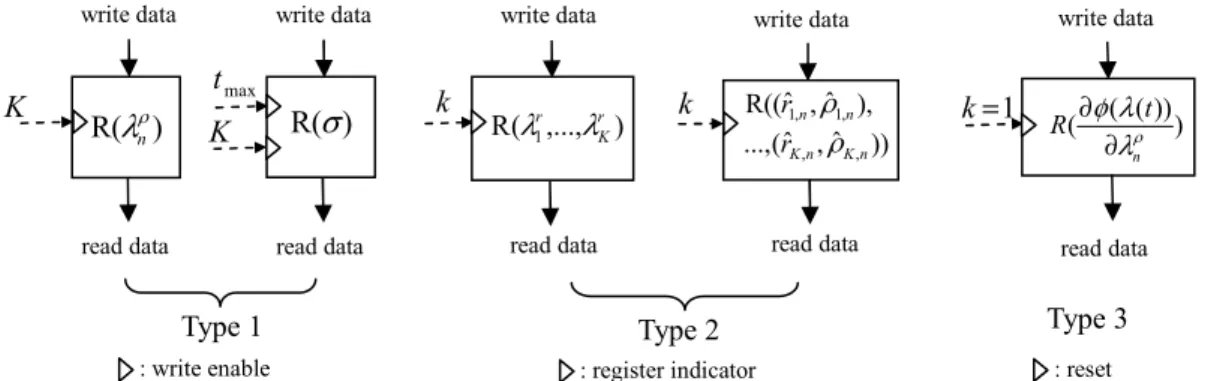
algorithm. For the sake of simplicity in interconnection, the registers for storing the constants are embedded in the PE responsible for the computations that need the constants. However, there are three types of registers denoted by R(∆)for storing the temporary computed-values of the variables ∆ as shown in Figure 3.1. For example, R(λρ_n) denotes the register for storing the computed value of λρ_n. The type 1 registers are for storing the computed values of

ρ

λn and σ ; λρn is updated when k=K, and σ is updated when both k=K and t=tmax

as indicated in Steps 7-8 and Steps 9-10, respectively. Therefore, a write enable controlled by the value of k and t are needed as shown in Figure 3.1. The type 2 registers are K-bank registers for storing the computed values of r ,k 1,...,K,

k =

λ or (rˆ_k,n,ρˆ_k,n), k =1,...,K, such that the kth bank will store the value of r

k

λ or (rˆ_k,n,ρˆ_k,n). Since the iteration index of the innest loop of the DPG algorithm is k, we need a register indicator k to point to the corresponding register bank as shown in Figure 3.1. Furthermore, r

k

λ and (rˆ_k,n,ρˆ_k,n) are computed for every k, thus type 2 registers are always write enabled. The type 3 register is for storing the value of ˆ 1

1 , −

∑

= k l n l

ρ ; therefore type 3 register is always write enabled, however its value has to be reset to -1 when k =1 as shown in Figure 3.1. It should be noted that the action of writing data into the registers occurs at the end of the clock pulse (i.e. at the positive edge of the next clock pulse) when write enable is active. For example, σ in _j R(_σ) is

updated to σ at the end of the clock pulse corresponding to both _j+1 k=K and t=t_max.

Figure 3.1. The three types of registers for storing the temporary computed values of the DPG algorithm. ) ( Rσ max t ) ,..., ( R 1 r K r _λ λ k ) )) ( ( ( _ρ λ λ φ n t R ∂ ∂ 1 = k )) ˆ , ˆ ( ..., ), ˆ , ˆ (( R , , , 1 , 1 n K n K n n r r ρ ρ k ) ( Rλnρ K write data read data write data read data write data read data write data read data write data read data

Type 1 Type 2 Type 3

: write enable : register indicator : reset

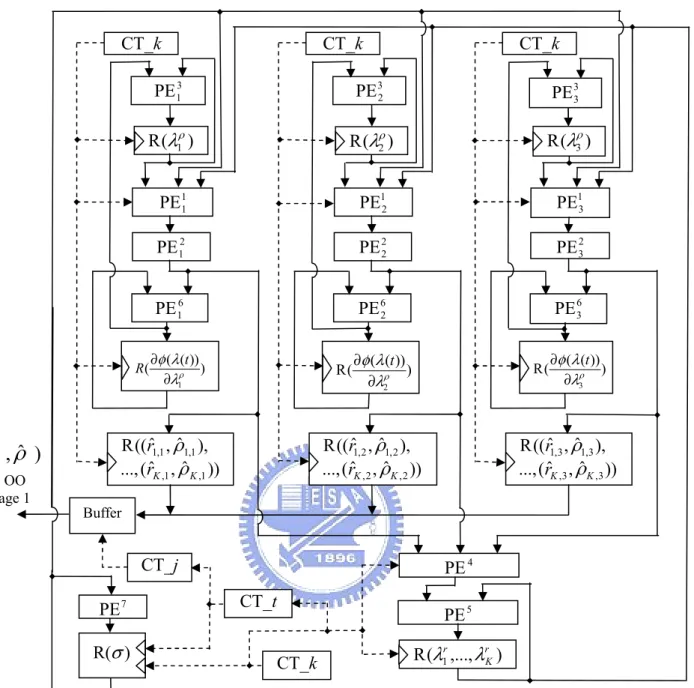
(ii) Regarding the computations, we employ seven types of PE to carry out all the arithmetic operations required in the DPG algorithm. These PEs are named as 1

n PE , 2 n PE , 3 n PE , _PE4_{, PE}5_, 6 n

PE , and _PE7_{, where the superscript denotes the type of PE, the subscript}

denotes the index of the array, and the PE without any subscript means it is single in the N PE arrays. Each type of PE consists of different hardware components needed for calculating a specific step in the DPG algorithm and yields the results needed in other step or steps. We will state the hardware components in a PE and its corresponding algorithmic step in the following. In the nth PE array, 1

n

PE performs Step 2 and outputs the computed (r~_k,n,ρ~_k,n) to 2 n

PE ;

its hardware components depend on the function f_k(c). In addition, 1 n PE consists of registers for storing 2 ,n k α and 2 , /

1 α_kn for all k and a register indicator k used to choose the corresponding register. 2

n

PE consists of six multipliers, four adders, and several comparators to perform Step 3 and output the computed (rˆ_k,n,ρˆ_k,n) to 6

n PE , _PE4 _{, and} ) ,..., 1 ), ˆ , ˆ (( R r_k,n ρ_k,n k = K ; 3 n

PE consists of a register for storing the constantβˆ_{, one adder and} one multiplier to perform Step 8 and output the computed λ_nρ(t+1) to R(λρ_n); 6

n

PE consists of one adder to perform Step 5 and output the computed

_∑

= − K k n k 1 , 1 ˆ ρ to ( ( _ρ( ))) λλ φ n t R ∂ ∂ and 3 n

PE . The single _PE4_{consists of log ( 1)}

2 N + adders to perform Step 4 and output the

computed _r k t λ λ φ ∂

∂ ( ( )) _{to the single PE}5_{. In addition, PE}4 _{consists of registers for storing} k

R

for all k and a register indicator k for choosing the corresponding register. The single _PE5

consists of a register for storing the constant β one adder and one multiplier to perform Step ˆ, 6; _PE5 _{outputs the computed} r_(t+1)

k

λ to R( ₁,..., r )

K

r _λ

λ . The single _PE7 _{consists of a}

register for storing the constant η and a multiplier to perform Step 10; _PE7_{outputs the}

computed σ(j+1) to R(σ).We summarize the characteristics of these PEs in Table 3.1 to

[to], and the computation complexity of a PE, which is shown in the last column and will be analyzed later.

Table 3.1

The characteristics of PEs

PE _{mic Step} Algorith Embedded _Constant Input Data [from] OutputData [to] Computation _Complexity 1 n PE Step 2 αk2,n,1/αk2,n )], ( R [ ) ( ρ ρ _λ λn t n )], ( R [ ) ( σ σ j )] ,..., ( R [ ) ( 1r rK r k t λ λ λ ] PE [ ) ~ , ~ ( 2 n , ,n kn k

r ρ 5⊗& 2⊕& 1ROM§

2 n PE Step 3 - (~r_k,n,ρ~_k,n)[ PE1_n] ˆ [ PE ],ˆ [ PE ], 6 n , 4 ,n kn k r ρ ) ,..., 1 ), ˆ , ˆ (( R [ ) ˆ , ˆ (r_k,n ρ_k,n r_k,n ρ_k,n k= K 2⊗ &1 ⊕ 3 n PE Step 8 βˆ )] ( R [ ) ( ], PE [ 1 ˆ 6 n 1 , ρ ρ _λ λ ρ n n K l ln t

∑

= − )] ( R [ ) 1 ( ρ ρ _λ λn t+ n 1⊗ & 1 ⊕ 4 PE Step 4 R_k ˆ [ PE ],...,ˆ [ PE2] N , 2 1 1 , kN k r r ( ( )) [PE5] r k t λ λ φ ∂ ∂ ) 1 ( log2 N+ ⊕ 5 PE Step 6 βˆ )] ,..., ( R [ ) ( ], PE [ )) ( ( 1 4 r K r r k r k t t λ λ λ λ λ φ ∂ ∂ )] ,..., ( R [ ) 1 ( ₁ r K r r k t λ λ λ + 1⊗ & 1 ⊕ 6 n PE Step 5 - ] PE [ ˆ )], )) ( ( ( [ 1 -ˆ 2 n , 1 1 , n k k l n n l t R ρ λ λ φ ρ _ρ

∑

− = ∂ ∂ ] PE ), )) ( ( ( [ 1 ˆ 3 n 1 , _ρ λλ φ ρ n k l n l t R ∂ ∂ −

∑

= 1⊕ 7 PE Step 10 η σ(j)[ R(σ)] σ(j+1)[ R(σ)] 1⊗

§_{⊗ : operation of a multiplication; ⊕ : operation of an addition; ROM: operation of accessing data of a ROM.}

(iii) There are three loops in the DPG algorithm, and the number of iterations in each loop has been set fixed. A branching will occur when completing the iterations of a loop as described in Steps 7, 9, and 11. Therefore, we need three counters to count the number of iterations consumed in each loop so as to control the branching of the DPG algorithm.

The three counters are the k-counter, t-counter and j-counter, denoted by CT_k, CT_t and CT_j, respectively, and represented by the square blocks shown in Figure 3.2. The values of CT_k and CT_t will be fed into the corresponding registers for proper operation. For example, the value k of CT_k will be used to indicate the iteration index of the innest loop, Steps 1-7, to point to the corresponding register bank in the Type 2 registers. When k=K,

there will be a branching at Step 7, such that the output data of 3 n

will be written into the register R(λρ_n). Similar reason applies to CT_t that when t= , t_max

there will be a branching at Step 9, such that the output data of _PE7_{, which performs Step}

10, will be written into the register R(σ Furthermore, when the value of CT_k changes ). from K to 1, the value of the register ( ( _ρ( )))

λ λ φ n t R ∂

∂ _{will be reset to -1 to perform Step 1. The}

value of CT_j will be used to detect the convergence of the DPG algorithm. Thus, when ,

max

j

j= the DPG algorithm will be stopped and output the approximate solution of (3.1), that is (rˆ_n,ρˆ_n),k=1,...,K ,n=1,...,N.

The counters are designed such that CT_k will circulate from 1 to K and increase by 1 for every clock pulse, CT_t will circulate from 1 to t_max and increase by 1 for every K clock pulses, and CT_j will increase by 1 for every K⋅t_max clock pulses.

(iv) Now, we are ready to interconnect the array PEs, registers and counters so as to execute the DPG algorithm. From the columns of the input data [from] and the output data [to] in Table 3.1, we can use solid lines with arrow heads to indicate the direction of the data flow to interconnect the PEs and registers as shown in Figure 3.3, in which we assume N=3 and do not show the system clock for the sake of simplicity.

The three counters, CT_k, CT_t and CT_j, as described previously, are used to count the number of iterations and control the branching of data flow. Therefore, to distinguish from the regular data flow, we use the dashed lines with arrow heads to indicate the flow of counter values to the corresponding registers as shown in Figure 3.3.

For the sake of simplicity, we will illustrate how the hardware architecture executes the DPG algorithm for one array as follows.

We initialize the values of registers ( ( _ρ( ))) λ λ φ n t R ∂ ∂ _{(Step 1:} ( ( ))_{) 1} ( =− ∂ ∂ ρ λ λ φ n t R ), R(λρ_n)

Figure 3.2. The three counters.