以車流模型為基礎之交通動態預測技術平台開發---子計畫一：動態旅次起訖推估與預測(II)

行政院國家科學委員會專題研究計畫 成果報告

子計畫一：動態旅次起訖推估與預測(II)

計畫類別： 整合型計畫 計畫編號： NSC94-2218-E-009-015- 執行期間： 94 年 08 月 01 日至 95 年 07 月 31 日 執行單位： 國立交通大學統計學研究所 計畫主持人： 周幼珍 報告類型： 精簡報告 報告附件： 出席國際會議研究心得報告及發表論文 處理方式： 本計畫可公開查詢

中 華 民 國 95 年 11 月 5 日

Dynamic Origin-Destination Estimation and Its Parallel

Implementation

Yow-Jen Jou, David Bernstein, Chien-Lun Lan

Abstract —Origin-Destination (O-D) information is important in many transportation

related domains, such as transportation planning, urban and regional planning, traffic

assignment, and so on. Historical studies assumed that the transition matrix is known

or at least approximately known, which is unrealistic for a real world network. To

obtain real-time O-D information in a reasonable way, state space model with Gibbs

sampler and Kalman filter is then introduced by researchers. The Gibbs sampler

method mentioned above requires considerable quantities of iterations and takes

massive computation time, thus parallel computing method has been introduced to

increase the computing power. This paper implements parallel computation for the

O-D estimation algorithm on a Linux cluster and gives a numerical example which

shows a satisfying result.

Keywords — dynamic origin-destination, state space model, Gibbs sampler, traffic,

PC cluster

1. Introduction

such as transportation planning, urban and regional planning, traffic assignment, and

even pedestrian simulation (Bernstein, 1996, 1997, 2001; Chang, 1994, 1999, 2004,

2005; Jou, 2001,2002; Gao 2002; Lee 2001). The O-D matrix provides a planner with

the basic information for planning a transportation system (Nanda, 1993). Traditional

ways of acquire actual O-D information can be obtained by an extensive traffic survey,

including license plate recognizing, automatic vehicle identification, and so on; this is

not only a cumbersome process but also very costly. Real-time O-D information,

which plays an important role in Intelligent Transportation System (ITS), is not

possible to obtain by the traditional method. With real-time O-D information,

numerous high-value ITS applications e.g., just-in-time delivery, time shortest path

emergency vehicle routing and congestion avoidance would be feasible. Due to this

reason, researchers have been seeking estimation methods to derive valuable O-D

flow information from less expensive traffic data, mainly link traffic counts of

surveillance systems. The existing studies on this subject can be roughly divided into

two categories: 1) Assignment-Based Methods and 2) Non-Assignment-Based

Methods (Chang, 1995).

The concept of assignment-based methods is mainly extended from static O-D

estimation method. These methods based on the assumption of reliable descriptive

appears to address the complex time-dependent issues in urban networks effectively,

if the descriptive model mentioned above exists and a time-series set of actual O-D

information is available. Another approach is the non-assignment based method. The

key concept of this approach is to assume that each O-D parameter remains

approximately constant during consecutive intervals of measurements. Researchers

proposed a variety of estimation methods in this subject, and the primary difference

among all recursive algorithms for dynamic O-D estimation lies in their unique way

of computing filter matrix. The main strength of non-assignment-based method is the

capability of providing O-D information from surveillance system which would be

relatively accurate and less expensive cost.

Jou introduced state pace model into dynamic O-D estimation which estimates

both O-D matrices and transition matrix simultaneously without any prior information

of state variables, while most of the aforementioned studies assume that the transition

matrix is known or at least approximately known, which is unrealistic for a real world

network. Gibbs sampler, a particular type of Markov Chain Monte Carlo (MCMC)

method, has been introduced in the solution algorithm to overcome the shortcoming

of the assumption of known transition matrix. The solution algorithm requires

considerable quantities of iterations and takes massive computation time, thus parallel

The remainder of this paper is organized as follows, the dynamic origin-destination

estimation (DODE) by state space model is introduced in section 2, the parallel

implementation of DODE is addressed in section 3, and the conclusion is outlined in

the last section.

2. Dynamic Origin-Destination Estimation

State space model is introduced to estimate O-D flow from link traffic counts.

The standard state space model is coupled with two parts: transition equations and

observation equations. First, the state equation which assumed that the O-D flows at

time t can be related to the O-D flows at time t-1 by the following autoregressive

form, n t u Fx x_t = _t−1 + _t, =1,2,3,..., (1)

wherex is the state vector which is unobservable, F is a random transition matrix, _t

( )

0,Σ ~ _p t N

u is independently and identically distributed noise term, where N _p

denotes the p-dimensional normal distribution, Σ is the corresponding covariance

matrix. x the state variable, is defined to be the path flow belonging to an O-D pair.

Next, the observation equation,

n t

v Hx

y_t = _t + _t, =1,2,3,... (2)

road network. The number of O-D pairs is denoted by p. H is a q× zero-one p

matrix, which denotes routing matrix for a network. v_t is also a noise term that

( )

0,Γ ~ _q t N

v . Both x and F are unobservable, thus Kalman filter is not suitable to

directly estimate and forecast the state vector. Hence, Gibbs sampler is used to tackle the problem of simultaneous estimation of F and x_t by latest available information.

There are two major elements to be incorporated in the solution method, 1)

filtering states by observations, and 2) sampling scheme of F and state variables. Since the observations y_t are not used in the conditional distribution, the Kalman

filter and the Gibbs sampler must be combined.

2.1 Kalman Filter

The Kalman filter is a system of recursions to estimate the state vector before a

new observation arrives, to forecast the observation, and to update the state vector as

the new observation is known. The structure of the filter can be derived in a Bayesian

framework as follows. The first stage (i.e. t =1), there’s no observation exists, thus the state vector x0 must be generated by a prior distribution that x0 ~Normal

(

µ0,V0

)

, where µ0 is the mean and V0 is the covariance matrix. By using equation (1), the

distribution for the state vector in the first stage will be normal with parameters

1 | 1 1

|

t t t t t

1 | 1 | 1

|

t t t t t t

Var x_⎣⎡ y_−⎦⎤=V ₋ =FV ₋F′+ Σ (4)

where µt t| 1− denotes the expect value of xt and Vt t| 1− denotes the variance of xt when yt−1 is observed. By the above information, the forecast observation would be

normal distribution with parameters

1 ˆ | 1 | t t t t t E y⎡_⎣ y₋ ⎤_⎦=y =Hµ ₋ (5) 1 1 | t t t t Var y_⎣⎡ y_{− ⎦}⎤=M =HV₋H′+ ϒ (6)

The above equation (3)-(6) holds for any t.

As the new observation yt become available, the parameter vector would be

updated according to Baye’s rule,

(

t| t

)

(

t| t

) (

t| t 1

)

p x y ∝ p y x p x y₋

by using Baye’s rule and standard Bayesian theory, the posterior will be normal

distribution with parameters

(

)

1 | | 1 | 1 | 1 t t t t Vt t H Mt yt H t t µ µ − µ − − ′ − = + − (7) 1 | | 1 | 1 | 1 t t t t t t t t t V =V ₋ −V ₋H M′ −HV ₋ (8)

The algorithm of Kalman Filter is illustrated as follows,

Algorithm Kalman Filter

Input:µ0, V0, yt:=observation sequence

Output: Filtered µ and V Begin

FOR each time step of the observation sequence Generate prediction of the new observation by

1

ˆ_{t t}

(

1

)

t t

M =H⋅ F V⋅ ₋ ⋅F′+ Σ ⋅H′+ ϒ Update the parameter by

(

)

1 | | 1 | 1 | 1 t t t t Vt t H Mt yt H t t µ µ − µ − − ′ − = + − 1 | | 1 | 1 | 1 t t t t t t t t t V =V ₋ −V ₋H M′ −HV ₋ END FOR END 2.2 Gibbs Sampler

The Gibbs sampler is a technique for generating random variables from a

distribution indirectly, without having to calculate the density. In this paper, we make the following assumptions, 1) The initial x0 ~N

(

µ0,V0

)

, 2) The covariance matrix Σ and ϒ are known, and 3) Given F, the distribution x_t is Gaussian.

The state equation can be written

1 t t t x′=x′₋F′+µ′, t=1,2,…,n that is 1 0 1 1 n n n x x F x x µ µ − ′ ′ ′ ⎡ ⎤ ⎡ ⎤ ⎡ ⎤ ⎢ ⎥ ⎢₌ ⎥ _′+⎢ ⎥ ⎢ ⎥ ⎢ ⎥ ⎢ ⎥ ⎢ ⎥ ⎢′ ′ ⎥ ⎢ ⎥′ ⎣ ⎦ ⎣ ⎦ ⎣ ⎦ M M M

The following notation is used for simplification. 1 n n x X x ′ ⎡ ⎤ ⎢ ⎥ = ⎢ ⎥ ⎢ ⎥′ ⎣ ⎦ M , 0 1 1 n n x X x − − ′ ⎡ ⎤ ⎢ ⎥ = ⎢ ⎥ ⎢ ′ ⎥ ⎣ ⎦ M , 1 n U µ µ ′ ⎡ ⎤ ⎢ ⎥ = ⎢ ⎥ ⎢ ⎥′ ⎣ ⎦ M , F′=

[

F′ _L F′ _L F′

]

Consider the element of the symmetric matrix

( )

{

_ij

(

_i, _j

)

}

(

) (

) (

)

(

) (

) (

)

(

)

( ) 1 ( ) 1 ( ) 1 ( ) 1 1 1 , ? ? ij i j n i n i n j n j n i n i n j n j i i n n j j S F F X X F X X F X X F X X F F F X X F F − − − − − − ′ ′ ′ = ′ − ′ ′ ′ − ′ ′ ′ ′ ′ ′ ′ ′ ′ ′ ′ ′ ′ ′ ′ = − − + − − where Fˆi

(

Xn 1Xn 1

)

1Xn 1Xn i( ) − − − −

′= ′ ′ is the least square estimate of F ′i , and Xn i( ) is

the i-th column vector of Xn. Consequently,

( )

(

i ?i

)

n 1 n 1

(

j j

)

S F′ = +A F′−F′′X − X′− F′−F′

where A is a p×p matrix, A=

{ }

aij with

(

( ) 1?

) (

( ) 1

)

ij n i n i n j n j

a = X′ −X′−F′′ X′ −X′−F′

That means, A is proportional to the sample covariance matrix. From the general

result in the Gaussian model, the posterior distribution of F ′ is then

(

)

( )

(

)

(

)

2 2 1 1 | , ? n n i i n n j j p F X S F F A F F X X F F − − − − ′ ∝ ′ − ∞ < ′< ∞ ′ ′ ′ ′ ′ ′ = + − − (9)

The distribution in equation (9) is a matrix-variate generalization of the t-distribution.

The following sampler for generating F ′ and X is then proposed.

Sampling Scheme Generate from the conditional distributions a. xt|F x, t−1,Σ~N Fx

(

t−1,Σ

)

b. | , ~

(

, ,

)

1 ( ) 2 1 1 2 1 1 2 p n n p n n n n F′ X Σ _⎣⎡k n p p ⎤_⎦− A − X − X′− A+FX − X′−F′−

The above sampling scheme would be the key component of the Gibbs sampler.

The Gibbs sampler is a Markovian updating scheme that proceeds as follows.

Given an arbitrary starting set of values Z₁(0),Z₂(0),Z₃(0),...,Z_k(0), and then draw

[

(0) (0)

]

3 ) 0 ( 2 1 ) 1 ( 1 ~ Z Z ,Z ,...Zk

visited in the natural order and a cycle requires k random variate generations. After i

iterations we have (Z₁(i),Z₂(i),Z₃(i),...,Z_k(i)) . Under mild conditions, Geman and

Geman showed that the following results holds(Robert, 1998).

Result 1 Convergence

[

k

]

i k i i i Z Z Z Z Z Z Z Z , , ,..., ) , , ,...,

( ₁() ₂() ₃() () → _{1 2 3} and hence for each s, ]Z_s(i) →[Z_s

as i→∞. In fact a slightly stronger result is proven. Rather than requiring that each

variable be visited in repetitions of the natural order, convergence still follows any

visiting scheme, provided that each variable is visited infinitely often.

Result 2 Rate

Using the sup norm, rather than the L₁ norm, the joint density of

) ,..., ,

,

(Z₁(i) Z₂(i) Z₃(i) Z_k(i) converges to the true density at a geometric rate in i, under

visiting in the natural order.

Result 3 Ergodic theorem

For any measurable function T of Z₁,Z₂,Z₃,...,Z_k whose expectation exits,

(

)

(

k

)

i l l k l l l i _i T(Z ,Z ,Z ,...,Z ) ET Z ,Z ,Z ,...Z 1 lim _{1 2 3} 1 ) ( ) ( 3 ) ( 2 ) ( 1 →

∑

= ∞ →

As Gibbs sampling through m replications of the aforementioned i iterations produces

k tuples

(

Z₁(i_j),Z₂(i_j),Z₃(i_j),...,Z_kj(i)

)

(

j=1,2,3,...,m

)

, which the proposed density estimate for

[ ]

Z having form _s

[ ]

=

∑

m₌

[

≠

]

j j r s s Z Z r s m Z 1 ) ( , 1 ˆ _.

variable forms the center part of the algorithm. In the process of generate state

variables, Kalman filtering mechanism is added. While a simple monitoring of the

chain (x(g)) can only expose strong non-stationarities, it is more relevant to consider the cumulated sums, since they need to stabilize for convergence to be achieved (Robert 1998). The solution algorithm with the time-complexity of

( )

2

O n is shown

as follows,

Algorithm Gibbs Sampler

Input: H:= path observation incidence matrix− , yt:=observation sequence Output: _Xˆ_{, F}ˆ Begin Initialize (0) : p F =I , Σ =: Ip, ϒ =: IP

{ }

store X = ∅ , Fstore= ∅

{ }

SET GibbsCount (g) to 0 WHILE not Converge

Generate ( )

(

)

~ , g x N µV Append ( )g x to Xstore

CALL Kalman Filter with µ, V , and observation sequence Generate F ′( g) by

{ }

( ) ) ( g ij g a A = ,

(

) (

(1) ( )

)

) ( ) ( ) ( ) ( 1 ) ( ) ( ) ( _{ˆ ˆ} g j g n g j n g i g n g i n g ij X X F X X F a = ′ − ′₋ ′ ′ ′ − ′₋ ′ Generate w~Wishart

(

X_n(₋g₁)X_n′₋(₁g),n−p

)

Generate Z =

(

z1′,z2′,z′3,...,z′p

)

,

(

)

) ( , 0 ~ p g iid k N A z COMPUTE F g w Z 1 2 1 ) ( − ⎟ ⎟ ⎟ ⎠ ⎞ ⎜ ⎜ ⎜ ⎝ ⎛ ′ ⎟⎟ ⎠ ⎞ ⎜⎜ ⎝ ⎛ = ′

APPEND ( )g

F ′ to Fstore

INCREMENT GibbsCount

END WHILE

READ last k items from Xstore and put in Xn

COMPUTE ˆ 1

n

X X

k

=

∑

READ last k items from Fstore and put in Fn

COMPUTE ˆ 1 n F F k =

∑

END

Accurate O-D information is difficult to obtain on a real road network, thus other

O-D information must be considered for validation. A numerical test of the DODE

algorithm with the real data has been conducted by Jou (Jou, 2003). The algorithm is

implemented on the Mass Rapid Transit network in Taipei, which consists of nine

stations. The results are generally satisfactory, showing that also in the unknown

transition matrix case, significant estimates could be obtained.

3. The Implementation of Parallel Computation and its Results

Computation power is crucial to achieve real-time information requirement, thus

the parallel computing technique is then been introduced to satisfy this requirement.

The solution algorithm should be modified to adopt the parallel implementation. It is

different random seed, each computing part will lead to a different solution chain. The

chain in each computing part will then be gathered to check the convergence. In this

situation, communication between computing nodes is minimum, and computing

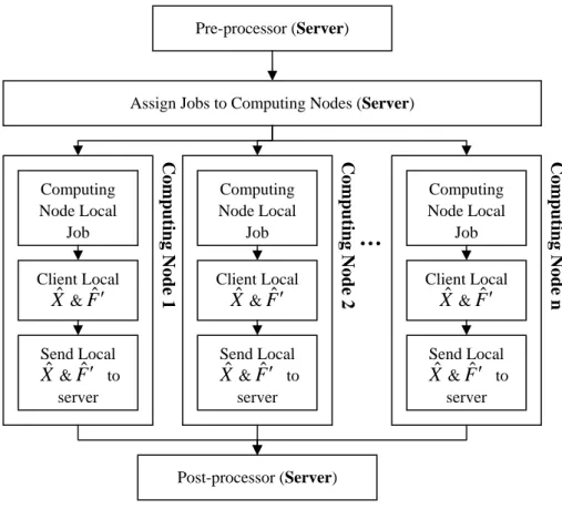
power can be easily increased without communication bandwidth limitation. Figure 1

describes the parallel architecture; a similar architecture had been proposed by Li (Li,

2002). In the pre-processor section, parameters used in our algorithm are initialized,

so does the necessary input data. When assign jobs, these input data are sent to

computing nodes in the cluster through TCP/IP base intranet with Message Passing

Interface (MPI) Library. The computational procedure for the parallel process consists

of:

Step 1. Load input data and parameters. Initialize MPI environment.

Step 2. Count the computing nodes exits in the cluster environment. Decide

the count of samples should be generated by each computing nodes.

Send data to each computing nodes.

Step 3. Each computing nodes generate its own _Xˆ _{and F ′}ˆ _{by given input}

data for given times. And then send the result to server.

Step 4. After all the data been sent to server, the server check the convergence

by each Xˆ and Fˆ ′ . If converge, the server estimate the global Xˆ

Step 5. Stop MPI environment. Output data.

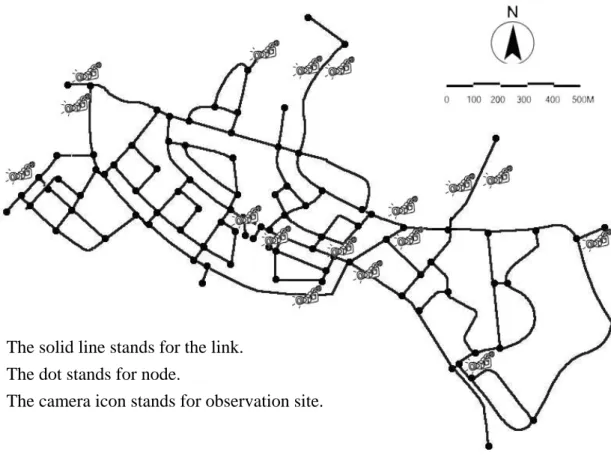
An empirical test is conducted on a part of real network located in Taiwan, the

HsinChu Science-based Industrial Park. The network is a closed network, with 11

entrances, which consists of 91 nodes and 244 links, shown as figure 2. There exist 17

observation sites on the network; the observation site updates traffic count every

minute.

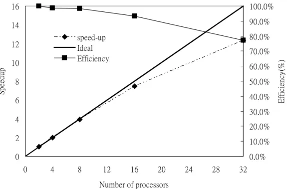
The parallel environment of this research consists of 16 computing nodes; each

contains 2 Intel XEON 3.2GHz processors and 1 GB memory. Nodes are connected

with a 1 Gigabits Ethernet switch for MPI protocol and a 100 Mbits PCI fast Ethernet

switch for Network File System (NFS) and Network Information System (NIS).

Figure 3 shows the speedups and efficiencies, where the speedups is the ratio of the

code execution time on a single processor to that on multiple processors and

efficiency is defined as the speedup divided by the number of processors(Gropp, 1999;

El-Rewini, 1998), of the parallel computing for 100 samples on the 32 CPU

Linux-cluster with MPI library. As shown in Figure 3, a quite good value of the

speedup and efficiency of the parallel scheme is achieved. That means we can

4. Conclusions

This paper introduced a dynamic origin-destination estimation method by state

space model. With Gibbs Sampler and Kalman filter, the algorithm loosens the

assumption of known transition matrix that exists in other studies. To satisfy the

real-time computation requirement of this algorithm, a parallel implementation on a

PC-based Linux cluster is conducted. The parallel implementation shows a good

result of nearly 80% of computing power remains for each CPU under a 32 CPUs

cluster environment. That leads to the conclusion: real-time estimation of O-D

matrices can be achieved by increasing a reasonable amount of CPUs.

Acknowledgement

This research was supported in part by the Ministry of Education of Taiwan, ROC

under Grants EX-91-E-FA06-4-4 and in part by the National Science Council of

Taiwan, ROC under Grants NSC-94-2218-E-009-015 respectively.

Authors

Yow-Jen Jou, Institute of Statistics, National Chiao-Tung University, Taiwan,

[email protected]

David Bernstein, College of Integrated Science and Technology, James Madison

Chien-Lun Lan, Department of Transportation Technology and Management, National

Chiao-Tung University, Taiwan, [email protected]

References

[1] C. K. Cater and R. Kohn, “Markov Chain Monte Carlo in Conditionally

Gaussian State Space Models”, Biometrika, Vol. 83, No. 3, pp.589-601, 1996.

[2] Christian P. Robert, “Discretization and MCMC Convergence Assessment”,

Springer, ISBN: 0-387-98591-3, 1998.

[3] D.A. bader, J. JaJa, R. Chellappa, “Scalable data parallel algorithms for texture

synthesis using Gibbs random fields”, IEEE Transactions on Image Processing,

Vol. 4, Issue 10, 1995.

[4] Daniel Sorensen, “Likelihood, Bayesian and MCMC methods in quantitative

genetics”, Springer-Verlag, 2002.

[5] David Bernstein, T.L. Friesz, Z. Suo and R.L. Tobin, “Dynamic Network User

Equilibrium with State-Dependent Time Lags”, Networks and Spatial Economics,

Vol. 1, pp. 319-347, 2001.

[6] David Bernstein, T.L. Friesz, “Infinite Dimensional Formulations of Some

Dynamic Traffic Assignment Models”, Network Infrastructure and the Urban

[7] David Bernstein, T.L. Friesz and R. Stough, “Variational Inequalities, Dynamical

Systems and Control Theoretic Models for Predicting Time-Varying Urban

Network Flows”, Transportation Science, Vol.30, pp.14-31, 1996.

[8] Gang-Len Chang, Xianding Tao, “Advanced computing architecture for

large-scale network O-D estimation”, Proceedings of the 6th 1995 Vehicle Navigation and Information System Conference, pp.317-327, 1995.

[9] Gnag-Len Chang, J. Wu, “Recursive estimation of time-varying

origin-destination flows from traffic counts in freeway corridors”, Transportation

Research 28B, pp.141-160, 1994.

[10] Gnag-Len Chang, X.D. Tao, “An integrated model for estimating time-varying

network origin-destination distributions”, Transportation Research, Vol. 33A

pp.381-399, 1999.

[11] H. El-Rewini, T. G. Lewis, “Distributed & Paralle Computing.”, Manning,

Greenwich, NY, 1998.

[12] Iljoon Chang, Gang-Len Chang, ”Calibration of Intercity Trip Time Value with a

Network Assignment Model: A Case Study for the Korean NW-SE Corridor”,

Journal of Transportation and Statistics, Vol. 5, 2002.

[13] Jodie Y. S. Lee, William H. K. Lam, and S. C. Wong, “Pedestrian Simulation

International Conference on Intelligent Transportation Systems, pp. 554-558,

2001.

[14] John H. Mathews, “Numerical Methods”, Prentice-Hall, ISBN: 0-13-626656-8,

1987.

[15] Pei-Yih Ting, R.A. Iltis, “Diffusion network architectures for implementation of

Gibbs samplers with applications to assignment problems”, IEEE Transactions

on Neural Networks, Vol. 5, Issue: 4, 1994.

[16] Pei-Wei Lin, Gang-Len Chang, Saed Rahwanji, “Robust Model for Estimating

Freeway Dynamic Origin-Destination Matrix”, Transportation Research Board,

2005.

[17] Pierre Bremaud, “Markov chains: Gibbs fields, Monte Carlo simulation, and

queues”, Springer, 1999.

[18] Raman Nanda, and Shinya Kikuchi, “Estimation of Trip O-D Matrix When Input

and Output are Fuzzy”, Proceedings of the IEEE International Symposium on

Uncertainty Modelling and Analysis, pp. 104-111, 2003.

[19] Song Gao, and Ismail Chabini, “Policy-Based Stochastic Dynamic Traffic

Assignment Models and Algorithms”, Proceeding of the IEEE International

Conference on Intelligent Transportation Systems, pp. 445-453, 2002.

Message-Passing Interface.”, MIT Press, Cambridge, MA, 1999.

[21] Yow-Jen Jou, Ming-Chorng Hwang and Jia-Ming Yang, “A Traffic Simulation

Interacted Approach for the Estimation of Dynamic Origin-Destination Matrix”,

IEEE International Conference on Networking, Sensing and Control, Vol. 2,

2004.

[22] Y. Li, S.M. Sze and T.-S. Chao, “A Practical Implementation of Parallel

Dynamic Load Balancing for Adaptive Computing in VLSI Device Simulation”,

Engineering with Computers, Vol. 18, pp. 124-137, 2002.

[23] Y.J. Jou, M.C. Hwang, Y.H. Wang, and C.H. Chang, “Estimation of Dynamic

Origin-Destination by Gaussian State Space Model with Unknown Transition

Matrix,” 2003 IEEE International Conference on Systems, Man & Cybernetics,

5-8 Oct. 2003, Washington, D.C., USA.

[24] Yow-Jen Jou, Ming-Chorng Hwang, “Rapid Transit System Origin-Destination

Matrix Estimation”, 2002 World Metro Symposium & Exhibition, Taipei, April

2002.

[25] Yow-Jen Jou, “Rapid Transit System O/D Pattern Calculation with Statistical

Gibbs Sampling and Kalman Techniques”, Conference on Computational Physics

Figure 1. The flow chart of parallel algorithm

Pre-processor (Server)

Assign Jobs to Computing Nodes (Server)

Computing Node Local Job Client Local Xˆ &Fˆ ′ Send Local Xˆ &Fˆ ′ to server Computing Node Local Job Client Local Xˆ &Fˆ ′ Send Local Xˆ&Fˆ ′ to server Computing Node Local Job Client Local Xˆ &Fˆ ′ Send Local Xˆ &Fˆ ′ to server

…

Computing Node 1 Post-processor (Server)

Figure 2. The test network.

The solid line stands for the link. The dot stands for node.

0 2 4 6 8 10 12 14 16 0 4 8 12 16 20 24 28 32 Number of processors Sp ee dup 0.0% 10.0% 20.0% 30.0% 40.0% 50.0% 60.0% 70.0% 80.0% 90.0% 100.0% E ffi ci en cy (% ) speed-up Ideal Efficiency