信用傳遞機制, 金融風暴與政府政策之總體經濟意涵

行政院國家科學委員會專題研究計畫 成果報告

信用傳遞機制, 金融風暴與政府政策之總體經濟意涵

研究成果報告(精簡版)

計 畫 類 別 ： 個別型 計 畫 編 號 ： NSC 98-2410-H-004-058- 執 行 期 間 ： 98 年 08 月 01 日至 99 年 10 月 31 日 執 行 單 位 ： 國立政治大學經濟學系 計 畫 主 持 人 ： 黃俞寧 計畫參與人員： 碩士班研究生-兼任助理人員：賴建男 碩士班研究生-兼任助理人員：何佩螢 碩士班研究生-兼任助理人員：林銘峰 博士班研究生-兼任助理人員：陳冠彰 博士班研究生-兼任助理人員：簡義哲 報 告 附 件 ： 出席國際會議研究心得報告及發表論文 處 理 方 式 ： 本計畫可公開查詢

中 華 民 國 100 年 01 月 21 日

行政院國家科學委員會補助專題研究計畫

 成 果 報 告

□期中進度報告

（計畫名稱）

信用傳遞機制, 金融風暴與政府政策之總體經濟意涵

計畫類別： 個別型計畫 □整合型計畫

計畫編號：NSC 98 － 2410 － H － 004 － 058

－

執行期間： 98 年 08 月 01 日至 99 年 10 月 31 日

執行機構及系所：政治大學經濟系

計畫主持人：黃俞寧

共同主持人：無

計畫參與人員：陳冠彰，簡義哲，賴建男，何佩螢，林銘峰

成果報告類型(依經費核定清單規定繳交)：



精簡報告 □完整報告

本計畫除繳交成果報告外，另須繳交以下出國心得報告：

□赴國外出差或研習心得報告

□赴大陸地區出差或研習心得報告

 出席國際學術會議心得報告

□國際合作研究計畫國外研究報告

Macroeconomic Implications of Policies under Financial Crisis

Yu-Ning Hwang1

Department of Economics

National Chengchi University

December 2010

ABSTRACT

The objective of this study is to examine quantitatively the macroeconomic implications of monetary and fiscal policies on the economy under a financial crisis. By using the model in Goodfriend and McCallum (2007) which introduces a banking sector in a dynamic stochastic general equilibrium (DSGE) model, we can investigate the effects of rescue policies in response to shocks to the credit market, the primary cause of the financial crisis. The model with money and banking permits the endogenous determination of various interest rates and the external finance premium, instead of one single interest rate in conventional settings. The calibration results are in line with the consensus recently reached by most economists. A fiscal policy which is large and is implemented rapidly can precipitate economic recovery better than the other way round. In addition, since the external finance premium declines with the implementation of the fiscal policy, it may dampen the crowding-out effects of expansionary government expenditure. On the other hand, the expansion in the high-powered money is more effective as a policy than the interest rate cuts. This is because the expansion in the base money increases bank reserves, facilitates deposits and encourages consumption, a mechanism that is absent from a model that neglects money and banking.

Keywords: Credit channel, Financial crisis, External finance premium

JEL Classifications: F13; F41; E42

1 *_{Yu-Ning Hwang is an Assistant Professor in the Department of Economics at National Chengchi} University, Taipei, 116 Taiwan. Comments are most welcome. Contact details: e-mail to

[email protected]; Tel.: 886-2-29393091 ext. 51641. I am grateful to Professor Tien-Wang Tsaur, Fu-Sheng Hung and all the participants in the Conference for the Financial Crisis and the seminar at the Central Bank of the Republic of China (Taiwan) for helpful comments and suggestions.

1. Introduction

The objective of this research is to examine quantitatively the effects of monetary and fiscal policies

under a financial crisis which was triggered by dysfunctional credit markets. A dynamic stochastic

general equilibrium (DSGE) model that includes the banking sector is established for policy analyses,

following Goodfriend and McCallum (2007). In this model, shocks to the credit markets can

characterize the current financial crisis that initiated from the credit markets. Equipped with the

adequate specification of financial shocks, this study conducts calibrations based on the US data to

evaluate the effects of different monetary and fiscal policies, in line with the current debates on

alternative specifications of rescue policies in reaction to the worst financial crisis since the Great

Depression decades ago. Moreover, while most economists’ arguments are based on earlier theories,

this study examines policies with a structural framework which offers a different angel to analyze

policies’ effects through numerical assessments.

The crisis broke out by the end of 2006 when the subprime mortgage default rates rose sharply after

the housing bubble burst in 2005. Starting from the beginning of this century, consecutive interest rate

cuts allowed banks to make loans to low-income families without the need to exercise prudent control

over the credit risks. These loans were funded by loan-backed securities which were available

worldwide. Aided by an extraordinarily easy monetary policy, investors could easily obtain funds with

high leverage for investments, and even on low-quality asset-backed securities. Therefore, the housing

crunch led to a chain of events: the value of the collateral for the mortgages fell, and this was

immediately followed by mounting default rates, which caused sharp declines in the values of the

underlying securities and in turn the asset markets as a whole. The slump in the values of the

During a financial crisis when markets fail to function normally, governments play an essential role

as Keynesian theory suggests. Initially, central banks all over the world implement expansionary

monetary policies by cutting interest rates, which can be performed both quickly and flexibly. However,

in contrast to normal times, the effects of interest rate rules seem to be limited in the event of a

financial crisis and fail to offset the recession that the crisis brings about. Hence, a massive fiscal

stimulus is needed. However, the specification of the policy is critical. The timing, size and priority

areas of the spending remain an open question.2

In the past decade, the DSGE model has served as the primary platform for the monetary policy

analyses of central banks all over the world. Nevertheless, while various asset market structures,

complete or incomplete, have been examined extensively under this framework, they are not the

primary cause of the current financial crisis. Therefore, it is crucial to include the credit market. It thus

seems to be natural to start from a model with a credit channel, which stresses the credit market’s

imperfections, as initially proposed by Bernanke and Blinder (1988), followed by Bernanke and Gertler

(1989, 1995), Bernanke, Gertler and Gilchrist (1998) and others. Bernanke and Gertler (1988) state that

rising interest rates, which are caused by a tightening of monetary policy, may worsen balance sheets,

raise agency costs and lead to higher loan rates for borrowers. The rise in the loan rate gives rise to a

higher external finance premium (EFP), which is the difference between the loan rate and the cost of

internal funds. As a result, the movement in the EFP can signal the asymmetric information problem in

the credit markets and exacerbate the downturn in economic activities. Therefore, the credit channel

serves as the financial accelerator of monetary policy, as has been illustrated by many studies. Edwards

and Vegh (1997), Kiyotaki and Moore (1997), Carlstrom and Fuerst (1997), Kocherlakota (2000) and

Cooley and Marimon (2004) have made substantial contributions to credit channel studies.

In line with the literature on the DSGE model and credit channels, the model presented in

Goodfriend and McCallum (2007) (henceforth, GM (2007)) offers a good platform to understand the

causes and transmission mechanism of financial crises which initiates from the credit market. The

model is essentially a combination of the DSGE model and the credit channel. While other models on

2

In a presentation at the January 2009 meeting of the American Economic Association, Feldstein (2009) stated that big and quick spending on increasing aggregate activity and employment is required.

the credit channel include real sectors only, GM (2007) highlight the role of money in an economy with

a banking sector. They argue that the omission of money would lead to the role of the demand for

money in facilitating transactions, which may attenuate the effects of the financial accelerator, being

neglected. On the other hand, it is also the first study to introduce the banking sector in a DSGE

model.3 In the model, the loan services that the banking sector offers require monitoring efforts and

collateral consisting of bonds and capital. As a result, the interest rates on the financial services and

assets, namely, the loan rate, bond rate, deposit rate and interbank rate, are endogenously determined.

The external finance premium (EFP) can be generated accordingly.

In this model, two shocks exist in relation to the credit markets, in addition to the productivity shock

to the production sector. One is the efficiency of the monitoring effort and the other is the effectiveness

of the collaterals for loans, which resemble the causes of the current financial crisis. GM (2007)

calibrates the model based on US data and finds that the EFP is generally countercyclical and that the

financial shocks do raise the EFP, thus signaling the rising agency costs in the market, which is

consistent with the credit channel literature. However, the calibration results also show that the EFP

may be procyclical in some cases due to the “financial attenuator” caused by the demand for money.

This model is good for the analyses on policies in response to the current financial crisis for several

reasons. First, the financial shocks they adopt in the model can well characterize the financial turmoil

that occurred since 2007. Second, the calibrations show that the rise in the EFP with the financial

shocks is in line with the data for the EFP since the beginning of this century, as shown below. Third,

this framework allows us to examine alternative fiscal and monetary policies. Differing from GM (2007)

which performs the analyses in order to understand the implications of the monetary policy for the

shocks, this study will focus on the effects of alternative monetary and fiscal policies in the event of a

financial crisis. In line with recent debates on the rescue policies in relation to the financial crises all

Two fiscal policies are proposed: one that involves a small but persistent amount of public spending,

and another that consists of a large amount of government spending that is less persistent. While both

of them are able to help the economy recover from the recession, the first policy causes the economy to

recover sooner than the second at the cost of drastic initial drops in consumption and investment. Due

to the initial decline in consumption, a massive amount of financial spending that takes place quickly

may be more desirable, as Feldstein (2009) points out.

Furthermore, it is worth pointing out that, while the importance of the credit channel to the monetary

policy transmission mechanism has been well recognized in the literature, no studies have performed an

examination of the transmission of fiscal policy based on the credit market paradigm. However, the

banking sector may play a significant role in the transmission of fiscal policy, similar to what it does in

the case of monetary policy. The calibration results in this model show that the EFP declines with the

government expenditure, and thus may offset the crowding-out effect of expansionary fiscal policy. The

decline in the EFP in this model does not imply the existence of a lower asymmetric information

problem (the moral hazard problem which is one of the main concerns in regard to large bailouts) under

fiscal policy, but demonstrates that the fiscal policy alters the demand for and supply of loans and

deposits, causing loan and deposit rates to move divergently.

Two monetary policies are examined as well, namely, the conventional monetary policy on the

control over the high-powered money and the interest rate rule. The calibrations show that the

expansion in the monetary base can boost the economy. The effect essentially comes from its direct

influence on the demand for money to facilitate consumption. The effect of the interest rate rule,

however, strongly depends on the persistence of the financial shock. If the credit market can be restored

quickly and thus more loans can be made out of the same amount of collateral, a small interest rate cut

is good enough for the economic recovery. On the contrary, persistent financial shocks nullify the

interest rate rule. This result may explain the fading effect of the interest rate since the crisis started.

Even if this model can serve as a good platform for policy analyses under a financial crisis, there are

certain restrictions due to the massive model structure. First, there are no defaults. The model

primary concern of bailouts. Thirdly, no study has so far incorporated fiscal policies into this framework.

characterizes the credit market imperfection by the decline in the effectiveness of capital as collateral

for loans, but there are no defaults for loans even if the value of the collateral has been low. While the

crisis may have been triggered by the surging default rates, this assumption seems to be unrealistic and

could be relaxed in future studies. Moreover, there are no investments. The capital in this model is thus

assumed to remain at the steady state level and the movements in investment are completely reflected

by the changes in the value of capital.

The remainder of this paper is organized as follows. In Section 2, we present the data on the EFP

from the beginning of this century, and the analysis illustrates that the EFP surged when the financial

crisis broke out. Section 3 outlines the specifications of the model. The dynamic analyses are listed in

Section 4 to discuss the dynamic responses of the macroeconomic variables in response to shocks to

policies and the financial sector, respectively. Several rescue policies for the financial crisis are

examined in Section 5. This analysis centers on the effects of fiscal policies of different sizes and

speeds as well as on alternative monetary policies. Section 6 concludes.

2. The significant movements in the EFP under financial crises

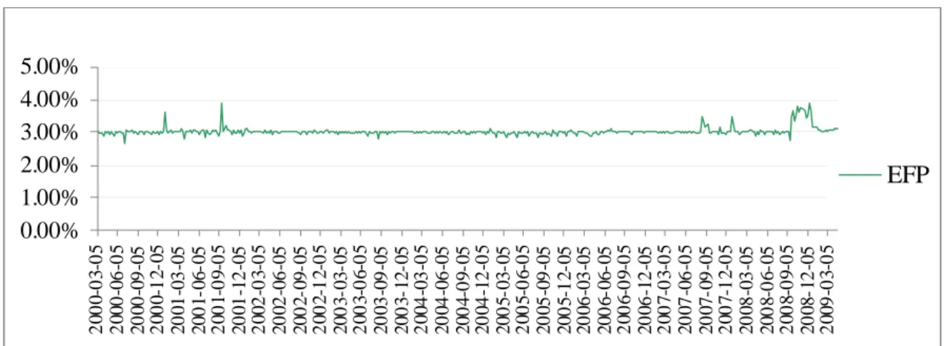
Fig. 1 lists the differences between the prime loan rate and the Federal funds rate5, which constitute the

external finance premium (EFP), in the early part of this century. While the EFP was fluctuating at

around the 3% level, it jumped up significantly in December 2000 and September 2001 after the

Internet bubble burst and the Enron scandal came to the fore. Similarly, the EFP also rose in August

2007 when the subprime crisis started to spread, followed by the sharp rise in mid-September 2008

after Lehman Brothers went bankrupt. While the Fed decided not to bail out Lehman Brothers, the EFP

Figure 1: The External Finance Premium

projects.

It is evident that the EFP rose sharply in times of financial distress, signaling the worsening of the

asymmetric information problem in the credit market. These times were

usually followed by economic recessions and thus were countercyclical as argued by Bernanke and

McCallum (1995). Therefore, it is important to use a model under which the loan and interbank interest

rates can be distinguished and the EFP is determined endogenously to capture the rising EFP after the

financial crisis and the asymmetric information problem that may exacerbate the downturn of the

economy after the financial crisis.

3. Model

The primary difference between this model and a typical DSGE specification is the inclusion of the

banking sector. In this model, consumers need to hold deposits in the bank for their own consumption,

and the bank can make loans. The loan services require real capital and marketable bonds as collateral,

along with labor input for credit monitoring. Therefore, households supply labor in both the goods and

banking sectors, and hold real capital for goods production as well as the collateral for loan services.

3.1 Goods Market 0.00% 1.00% 2.00% 3.00% 4.00% 5.00% 20 0 0 -0 3 -05 20 0 0 -0 6-05 20 00 -0 9 -0 5 20 0 0 -1 2 -0 5 20 01 -0 3 -0 5 20 0 1 -06-0 5 20 0 1 -0 9 -05 20 01 -1 2 -0 5 2 002 -0 3 -0 5 20 02 -0 6 -0 5 20 0 2 -09-0 5 20 0 2 -1 2 -05 20 0 3 -03-0 5 20 0 3 -0 6 -05 20 03 -0 9 -0 5 20 0 3 -12-0 5 20 0 4 -0 3-05 20 04 -0 6 -0 5 20 0 4 -0 9-0 5 20 04 -1 2 -0 5 20 0 5 -03-0 5 20 0 5 -0 6 -05 20 05 -0 9 -0 5 20 0 5 -1 2-0 5 20 06 -0 3 -0 5 20 0 6 -06-0 5 20 0 6 -0 9 -05 20 06 -1 2 -0 5 20 0 7 -0 3 -05 20 07 -0 6 -0 5 20 07 -0 9 -0 5 20 0 7 -1 2 -05 20 08 -0 3 -0 5 20 0 8 -0 6-0 5 20 0 8 -0 9 -05 20 08 -1 2 -0 5 2 009 -0 3 -0 5 EFP

Since the goods market is assumed to be monopolistically competitive, a typical consumption bundle

consists of a variety of differentiated goods, formed according to the Dixit-Stiglitz composite

consumption index with  as the elasticity of substitution. The aggregate consumption index and the associated aggregate price level are shown below:

1 1 ₁ 0 i t t C C di   _   _      



 , 1 1 1 1 0 t i t P P di     _ _ 





Accordingly, the demand function for each individual good is:

i i t t t t P C C P         

where C_ti and P_ti are the consumption and price of good i , and C_t and P_t are the aggregate

consumption and price indices. Goods can be used for consumption, capital investment and government

expenditure. The aggregate capital good, K_t, and government spending, G_t, which are also composed

of a variety of goods, are assumed to follow the same composition as the consumption goods.

The firm employs labor and capital for the production of goods and its productivity is subject to

exogenous shocks. Thus, under monopolistically competitive markets, the goods market clearing

condition for a typical good j can be written as:





1





j P dj j t t t t t t

K  A l  AD P P  (1)

where A_tp denotes the productivity shock and  denotes the share of capital in production. AD_t

represents the aggregate demand in the economy which can be written as C_tq I_{t t} , where G_t  is

the depreciation rate, I_t K_t1 



1 



K_t and q_t is the market price of capital. Therefore, the profit of a typical firm,  , can be stated as: _tFj

1

j

P 

To simplify the model, the capital stock is assumed to remain at the steady-state level, which is

endogenously determined. Therefore, in each period, goods are invested simply for making up

depreciation. While capital remains constant at the steady state level, q_t is the essential factor that

determines the investment movements.

3.2 Households

The representative individual household obtains utility from the consumption bundle and labor supply:

1 

_

_{ }

_





0 0 1 1 log 1 t i si si t t t t E  C    l n     _{    }   



 where s t

l and n are labor supplies in the production and banking sectors, respectively. _ts  is the subjective time preference. The budget constraint for the household can be written as:









_

_





1 1 ₁ 1 1 1 i D di L di i i di di t t t t F i t si si i t i t t t t t t t t t t B t t t t t t t t R D R L B B D L q I w l n r K C T P P P P R P   _   _              (2)

Households hold two types of assets, bonds B and demand deposits _t D . The interest rates associated _t

with the bond and deposit are R and _tB R respectively._tD 6 In addition, they borrow from the bank L _t

at the loan rate R . The superscript _tL d is used to denote the demand of the assets from the households.

t

T is the lump-sum tax.

Here, household faces the deposit-in-advance constraint, which is binding every period: i i t t t D C P   (3) where  is a constant, reflecting the assumed rigidity, and D denotes the nominal deposit. _t

6

As shown below, the balance sheet of the bank shows that H_t D_t in equilibrium, where the central bank acts as L_t

the reserve supplier. Together with the profit functions of the firm and bank, we can obtain the individual budget constraint in GM (2007).

3.3 Bank

The balance sheet for a typical banking sector is:

t t t

H L D (4)

where H is the reserve that the bank holds toward the deposit and _t L represents the bank loans to _t

households. Assume  is the reserve ratio, thus H_t D_t and L_t  



1 



D_t. The loan service is provided by using labor for monitoring and collateral, which consists of the bonds and capital that the

household holds. The loan production function can be written as:



 



1 1 1 , 0 1 k n t t t t t t t t L P F b A mq k A n           (5)

where b_t1B_t1 P_t



1R_tB



and  is the fraction of the collateral takes in the loan production. F characterizes the overall efficiency of the loan production and a higher value of F stands for more

efficient loan making which incurs lower marginal cost. 0 m 1 indicates that real capital embeds higher risk and is less efficient than bonds as collateral.7 A and _tk A are shocks to the collateral and _tn

monitoring efforts, respectively. The negative A indicates the financial distress resembling the _tk

current crisis which was triggered by the decline in the housing price, the collateral for mortgage. A

negative shock to A , on the other hand, describes the lack of monitoring for loans. _tn

3.4 Government

The government budget constraint can be written as:



1



1



1



B

t t t t t t t t t t

3.5 Optimality Conditions

Under the model specifications, household i , as a worker and firm, chooses the variables l , _tsi l , _ti n , _tsi

i t

n , K_ti_1, P and _ti B_ti_1 to maximize her utility, subject to the constraints, Eq. (1) and (2), with the

multiplier _t and _t respectively. The associated first-order conditions are similar to those in GM (2007), except for the nonzero G . With the banking sector, the first-order conditions differ from those _t

in conventional settings in the role of bonds and capital, which function as the collaterals for loans and

thus provide additional liquidity services for households. Let



1 1



k

t Ct bt A mq Kt t t

   (7) Then the Euler equation associated with the bond can be derived as the equation below:





1 1 1 1 1 B 0 t t t t t t t t t C P E R P   _                         (8)

The first term of the Eq. (8) stands for the loans that one unit of the bond can support. Similarly, the

capital also yield similar liquidity service, and thus the condition with respect to capital possesses the

additional term in the front:





1 1 1 1 1 1 1 1 1 1 0 t t t t t t t t t t t t t t C A l m q q E q K    _{ }  _                                  _   _     _   _ (9)

Since all the individuals are assumed to be identical, P_ti  and the superscript i is dropped for all P_t

variables.

3.6 Interest rates

There are four interest rates in the overall credit markets. Because these interest rates are associated

with the consumption, labor supplied, and the costs that the liquidity services incur, these

corresponding interest rates are endogenously determined by the optimizing behaviors of consumers

is the interest rate in the conventional general equilibrium model without banking, is treated as the benchmark rate: 1 1 1 T t t t t t t P R E P  _   (10)

Therefore, the difference between the bond rate and the uncollateralized rate can be obtained by

combining Eq. (8) with Eq. (10)





1 B 1 t 1 1 T t t t t C R R           _{ }  _{ }      (11)

Other interest rates that are associated with the operation of the banking sector will involve the real

marginal costs that the operation incurs. Since the Federal funds market is the primary source of funds

for the bank, the interbank rate R is the cost of the fund for the bank to make loans. Therefore, when _tIB

the bank loans the funds out, uncollateralized or collateralized, the interest rates have to cover the real

marginal cost that the loan process requires. Without certain conditions such as collateral or credit

checks, the uncollateralized rate R has to cover the interbank rate and the real marginal cost that is _tT

associated with the loan process which is w n_{t t}





1



1



C_t



and thus the relationship between the interbank rate and the uncollateralized rate can be expressed as:



1



1

_

_

_



1



1 1 IB t t T t t t w n R R C       _  _      (12)

On the other hand, the real marginal cost of the collateralized loans is w n_{t t}





1



C_t



which is the partial derivative of the loan services with respect to n . The primary difference between the marginal _t

cost of collateralized and uncollateralized loans lie in



1



, the share of monitoring in the loan process which can effectively reduce the marginal cost. Thus, the collateralized rate R can be written _tL

relationship between the interbank rate and the deposit rate can be written as:



1



D IB t t

R R  (14)

Thus, from Eq. (13), we can obtain the EFP, which expresses the spread between the bank’s external

and internal interest rates as a function of endogenous variables9:



1



L IB t t t t t t w n EFP R R C       (15)

The real marginal cost of loan supply, as indicated by GM (2007), is determined by the endogenous

variables C , _t m , _t w , and the parameters associated with the loan production. Therefore, while the _t

government’s monetary and fiscal policies affect consumption, labor and the wage, they also alter the

EFP that the household undertakes.

3.7 Nominal rigidity

While the prices are flexible in the long run, we assume that prices are rigid in the short run and that

firms adopt Calvo staggered pricing as the pricing strategy. Without specifically specifying the firms’

optimal pricing, the price adjustment process is characterized as follows:

 p_t E p_t _t1_t (16) u_t where   and 0 1 log( ) log( ) t t t p P P_    (17)

which stands for the inflation rate of the aggregate price level. _t denotes the real marginal cost of goods production and can be identified as:

t t t

   (18)

3.8 Exogenous shocks

The exogenous shocks, A and _tP A , are assumed to follow a constant growth rate _tn  in the long run

9

Since the interbank rate is only slightly lower than the deposit rate due to small  , here the interbank rate is used for the derivation of EFP.

but to fluctuate in the short run. The shock to the efficiency of capital as the collateral, however, is

assumed to be stationary. Since the cause of the financial crisis is the dysfunctional credit market

caused by lower efficiency in loan production, the following analyses will focus on the impacts of the

unit shocks A and_tk A . The detrended (trendless) shocks are assumed to follow an AR(1) process: _tn

1 k k k t k t t e  e_   1 n n n t n t t e  e_  

where _tk, _tn are iid random variables and _k, _n indicate the persistence of these shocks, both of which are specified as 0.95 for the dynamic analyses to capture the slow recovery speed of the credit

markets that is subject to financial innovations and restoration.10 Since the effects of the shocks A _tk

and A on the economy are quite similar, we will discuss only the cases under the shock to the _tn

effectiveness of collateral e . _tk

3.9 Policies

The crucial part of the calibration is the specification of policies. The government will respond to the

financial shocks through interest rate cuts, expansion in monetary base, or expansionary government

expenditure. As for the monetary policy, we propose two types of monetary rules. The central bank

takes control over the interbank rate R : _tIB



1 3



0



1 1



2 3 1 ,

IB IB k

t t t t R t R t

R   _    p   _ R_ D e e (23)

financial distress on the economy with the magnitude of D in response to a unit shock to _R e . The _tk

interest rate cut implies that the value of D should be negative. _R

In addition to the Taylor rule, an alternative monetary policy that involves controlling the growth rate

of high-powered money is also discussed. Although most central banks all over the world regularly

implement the interest rate rule, the financial crisis has forced governments to adopt the “quantitative

easing” strategy by providing the markets with abundant liquidity. The rule is stated below:

m_t _mm_t1e_{m t,} D e_{m t}k (24)

where m_t log

 

H_t log



H_t1



which is the growth rate of the monetary base. Under this policy, the interbank interest rate is endogenously determined. e_{m t,} is the shock to the stock of money, and D _m

stands for the central bank’s response to the shock which should be positive.

As for the fiscal policy, we assume that the government will respond to the shock by increasing the

government expenditure, which is assumed to be an exogenous process:



1



1 ,

k t g g t g t g t

G   G G_ e D e (25)

where G is the steady state value of the government expenditure, _g states the persistence of the temporary spending, and e_{g t,} is the government spending shock. In a similar fashion, D _g

characterizes the magnitude of the government spending in response to the shock and thus should be

positive. The government can finance the spending by issuing bonds, money or increasing taxes. To

obtain the equilibrium, we will need to exogenously specify one of the fiscal policies, the process of

issuing bonds or levying taxes, leaving the other to be endogenously determined. In the calibrations

below, we assume that the government maintains the ratio of bonds to consumption, _t, stationary: _t  



1    _b



 _{b t1}e_{b t,} (26)

where e is the current shock to the bond-consumption ratio._{b t,} 12

12

In future studies, we may relax this assumption by merely levying the income tax, thereby leaving the quantity of outstanding bonds to be endogenously determined.

3.10 Equilibrium

The sticky-price equilibrium which is constituted by C , _t l , _t n , _t P , _t w , _t q , _t B , _t T , _t D , _t L , _t R , _tB

t

 , _t, _t,  and p_t  can be obtained by solving Eq. (1)-(13), (20)-(22) under exogenous _t

specifications of monetary policy (24) and the fiscal policy (25) and (26). In turn, R along with all _tIB

other interest rates can be determined by Eq. (15)-(18). Nevertheless, the equilibrium of an economy

where the central bank exercises the interest rate rule can be characterized by replacing the monetary

policy rule Eq. (24) with the interest rate rule Eq. (23).

In the calibrations, the steady state is assumed to be deterministic where shocks are absent and can

be obtained by solving the system under flexible prices.13 The dynamic analysis is performed through

loglinearization with respect to the endogenous variables around the steady state, with some parameters

being chosen to match certain features of the steady state values.

4 Dynamics

Before proceeding further with the examination of the policies under the financial crisis, Section 4 lists

the impulse response functions for each shock: _,, _,, k g t m t t

e e e , respectively. The calibration results in this

section illustrate the implications of money and banking for the policies and the financial shocks. The

discussion in this section will help us better understand the implications of the policies for the financial

crisis, how they should be implemented and their effects.

quarterly data in the US.14 Differing from GM (2007) in which case there was an absence of

government expenditure, public spending is assumed to be 0.22 in the steady state in order to capture

the share of government spending in GDP as 20%, following Schmitt-Grohe and Uribe (2002). The

ratio of bonds to consumption in the steady state is assumed to be equal to 0.56.  0.38 is calibrated to obtain the steady state labor supply, which is approximately equal to 1/3 after the government

expenditure is added.15 The steady-state money stock is chosen by letting the aggregate price level be

equal to one. In addition, while the value of capital is allowed to fluctuate in the short run, it is assumed

to be one in steady state, q . The growth rate of exogenous shock is specified as 1  0.005. The elasticity of substitution  is assumed to be equal to 11 to capture the markup of 1.1 for the monopolists. Following the conventional setup, we assume  0.99,  0.36 for the capital share in production and  0.025 to capture the quarterly depreciation rate. The parameters in the banking sector are specified as those calibrated in GM (2007). In the banking sector, GM (2007) calibrate US

data and find that  0.31, 0.65, m0.2 and  0.005. F 9 is calibrated to characterize the inefficient production in the banking sector which results in nonzero marginal costs.  is assumed to be equal to 0.02 as the recent literature indicates.

4.2 Unit shock to the government expenditure

14

The large scale of the model is another reason and thus the choice of parameters is relatively restricted. An alternative specification of the parameters may generate negative steady-state values or multiple equilibria.

15

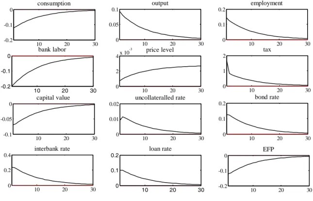
10 20 30 -0.2 -0.1 0 consumption 10 20 30 0 0.05 0.1 output 10 20 30 0 0.1 0.2 employment 10 20 30 -0.2 -0.1 0 bank labor 10 20 30 0 2 4x 10 -3 _{price level} 10 20 30 0 1 2 tax 10 20 30 -0.1 -0.05 0 capital value 10 20 30 0 0.01 0.02 uncollateralled rate 10 20 30 0 0.1 0.2 bond rate 10 20 30 -0.2 -0.1 0 EFP 10 20 30 0 0.1 0.2 loan rate 10 20 30 0 0.2 0.4 interbank rate

Fig. 2: 1% increase in government expenditure, g t_, 0.01.

To examine the effects of fiscal policy on an economy with money and banking and highlight the role

of money and banking in the dynamic responses of macroeconomic variables to expansionary

government spending, here we calibrate the model with a unit shock to the government expenditure. It

is conducted based on the interest rate rule with the policy parameters being specified as:₁0.15,

2 0.5

  and ₃ 0.95.

Fig. 2 shows that employment in the production sector rises by 0.14% in response to a 1% point

increase in the government expenditure, resulting in a 0.09% increase in output, which is slightly lower

than 1%. The rising aggregate demand causes the price level and all the interest rates to increase with

the expansionary government expenditure as the Keynesian theory suggests. The increased interest

rates result in crowding-out effects on output by lowering consumption and the price of capital,

10 20 30 0 0.5 consumpion 10 20 30 0 0.5 output 10 20 30 0 0.5 1 employment 10 20 30 40 -1 -0.5 0 bank labor 10 20 30 0 5 10 price level 10 20 30 0 0.5 1 inflation rate 10 20 30 0 0.5 1 capital value 10 20 30 0 0.5 1 uncollateralled rate 10 20 30 0 2 4 bond rate 10 20 30 0 2 4 interbank rate 10 20 30 0 1 2 loan rate 10 20 30 -0.5 0 0.5 EFP

Fig. 3: 1% increase in the high-powered money, m t_, 0.01.

ˆ _{ˆ ˆ ˆ}

EFP  w m c. While m, w and c are all reduced, the decrease in consumption

dominates. If the investment and consumption in the economy can be financed externally, the lower

EFP will raise the level of investment as well as consumption, thereby offsetting the crowding-out

effect of government expenditure. As a result, the drops in consumption and investment are relatively

moderate, being 0.12% and 0.07%, respectively.

Therefore, a model which neglects banking and money may overstate the crowding-out effect of the

fiscal policy. While the public spending crowds out consumption, the demand for deposits is lowered,

which should be accommodated by the proportionate drop in the loan. However, the lower demand for

the loan is offset partially by the decreases in investment and employment in the banking sector which

are crowded out by the expansionary government spending. The smaller magnitude of the loan rate rise

reduces the EFP.

4.3 Unit shock to the growth rate of high-powered money

accelerator in the transmission mechanism of monetary policy, which is mainly caused by the balance

sheet effect. The exclusion of money in the conventional credit channel literature, however, may

neglect the impact of the demand for money on the EFP that may in turn attenuate the influences of the

financial accelerator, as argued by GM (2007).

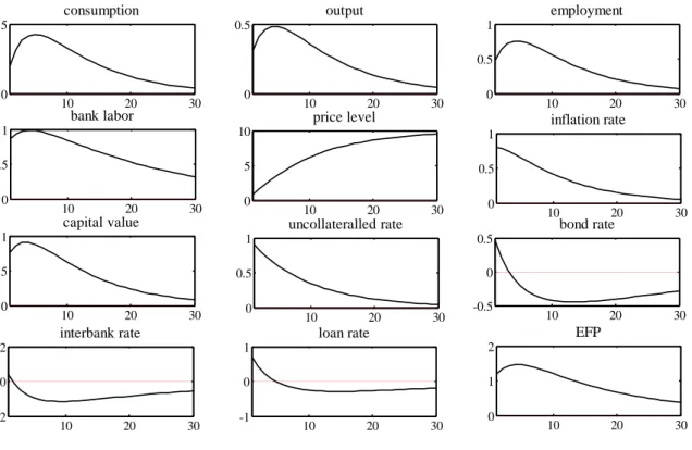
The mixed effects of the expansionary monetary policy on the EFP are evident in Fig. 3. With the

calibration on the high persistent growth of money _m0.9, the 1% increase in the growth rate of money causes the EFP to drop initially, to rise afterward to a level above the steady state value, and

then to decline gradually to the normal level. The initial drop, which is countercyclical, may be viewed

as the “financial accelerator” as in Bernanke & Gertler (1995), but the positive levels in the following

periods represent the “financial attenuator” as referred to by GM (2007).

Except for the movements in the EFP, all other variables are consistent with the results that GM

(2007) report. Consumption increases by 0.44% and output rises by 0.48%. The economic boom drives

up the inflation as well as q , whose effects die away gradually after 2 quarters. _t

4.4 Unit shock to the effectiveness of collaterals

Before implementing policies under the financial shock, we need to understand how the financial shock

impacts the economy. The calibration results are listed in Fig. 4. Most of the results here coincide with

the results that GM (2007) report. Consumption, output and employment decrease upon the impact of

10 20 30 -0.1 -0.05 0 price level 10 20 30 -0.01 -0.005 0 inflation rate 10 20 30 -0.05 0 0.05 capital value 10 20 30 -0.05 0 0.05 uncollateralled rate 10 20 30 -2 -1 0 bond rate 10 20 30 0 1 2 EFP 10 20 30 -1 -0.5 0 loan rate 10 20 30 -4 -2 0 interbank rate 10 20 30 0 1 2 bank labor 10 20 30 -0.1 -0.05 0 consumption 10 20 30 -0.1 -0.05 0 output 10 20 30 -0.1 -0.05 0 employment

Fig. 4: 1% shock to the effectiveness of collaterals, _tk  0.01.

to drop sharply on impact, and then adjust gradually back to the steady state without any

policy assistance. The recession is accompanied by deflation. This is consistent with what is usually

observed after the financial crisis strikes. Most of the interest rates decrease as well, except for the

uncollateralized rate.16 The increase in R may, however, mislead the reactions of governments. In a _tT

model that does not distinguish between interest rates, R is the only interest rate that guides the _tT

consumption and investment decisions of households and firms. In a model where external financing

for private spending is likely, however, R and _tL R are the crucial determinants of consumption and _tB

saving behavior. While their movements diverge, the interest rate rule of the central bank that views

T t

R as the benchmark interest rate may be misleading. This finding illustrates the importance of money

and banking for policy making.

The EFP rises upon the shock, consistent with the statement of Bernanke & Gertler (1995) the EFP is

countercyclical and characterizes the worsening asymmetric information problem under the crisis. The

16

countercyclical EFP will cause the credit to contract, thereby delaying the recovery of the economy.

The value of capital, q , decreases at the outbreak of the shock, but rebounds rapidly to a level that is _t

greater than the steady state in one quarter, because the decline in interest rates raises the discounted

sum of the future marginal product of capital. Notwithstanding the initial decline in capital value is

close to that in the real world, the speed of recovery seems to be too fast. A possible reason that

accounts for the rapid adjustment of q is the frictionless capital market where there is no price _t

stickiness or costs that the capital adjustment may incur.

5 Policies under the financial crisis

Based on the above discussions, the policies under the financial crisis will be examined. In this section,

we let _tk  1% in all cases and policies are allowed to react to the financial shock. Instead of determining the optimal monetary and fiscal policies, this section will investigate the effects of various

policies on the dynamic responses of the economy and whether they can precipitate the economic

recovery. In particular, the assessment in this section will center on the sizes and speeds of various

policies. The results reveal that large and rapid government expenditure performs better than small and

persistent government expenditure. On the other hand, while an expansionary monetary policy will help

the economy recover from the crisis, the effects of the interest rate rule crucially depend on the

persistence of the financial crisis. The results correspond to Feldstein’s suggestions on the format of

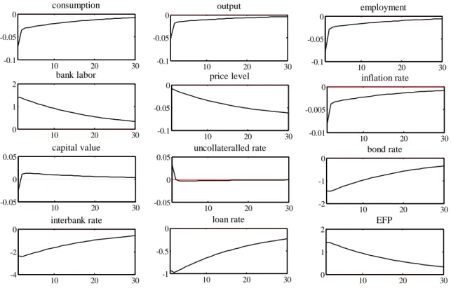
10 20 30 -0.2 -0.1 0 consumption 10 20 30 0 0.05 0.1 output 10 20 30 0 0.05 0.1 employment 10 20 30 0 0.5 1 1.5 bank labor 10 20 30 -0.06 -0.04 -0.02 0 price level 10 20 30 0 1 2 3 tax 10 20 30 -1 -0.5 0x 10 -3 _{capital value} 10 20 30 -0.05 0 0.05 uncollateralled rate 10 20 30 -1.5 -1 -0.5 0 bond rate 10 20 30 0 0.5 1 1.5 EFP 10 20 30 -3 -2 -1 0 interbank rate 10 20 30 -1 -0.5 0 loan rate

Fig. 5: small but persistent government expenditure:D_g 1 and _g 0.9.

rules. As a result, this study can also serve as a justification for the large public spending

policies that most governments all over the world are currently implementing while the effects of

interest rate rules die away quickly or are even not strong enough to offset the impacts of the crisis.

5.1 Fiscal policy

Two fiscal policies are examined in this section: a stable government expenditure plan, which is small

but persistent, and a drastic cure policy, which is large and less persistent. While the first one stands for

normal government expenditure, the second one is conducted to find support or objections to the recent

policy plans that most economists have proposed for the economy to recover from the recession

following the financial distress.

5.1.1 Small and persistent government expenditure

Here we propose a highly persistent government expenditure and allow the public spending to react

100% to the financial shock. Therefore, D_g  and 1 _g 0.9. Similar to Section 4.2, the examination of the fiscal policy is conducted under the persistent interest rate rule. The effects of the expansionary

fiscal policy are evident by comparing Fig. 4 and Fig. 5. As shown, the implementation of the

government spending can successfully help the economy avoid recessions. Output increase by 0.06%

instead of -0.05% when there is no public spending.

However, there is no free lunch. The expansionary public spending makes consumption drop, instead

of increasing, by 0.19% and the investment decline by 0.1%, compared with the earlier levels before

the policy was implemented of -0.07% and 0.013%, respectively. The increase in the aggregate demand

leads to a rise in interest rates and the crowding-out effects.

Nevertheless as output and interest rates rise, the EFP is lowered but remains above the normal level

and thereby becomes procyclical. This may dampen the crowding-out effect of expansionary fiscal

poliy as discussed. Differing from the “financial attenuator” in GM (2007), the procyclical EFP is

caused by the expansionary fiscal policy which drives up the output, but is not strong enough to push

down the EFP to the level below the steady-state value.

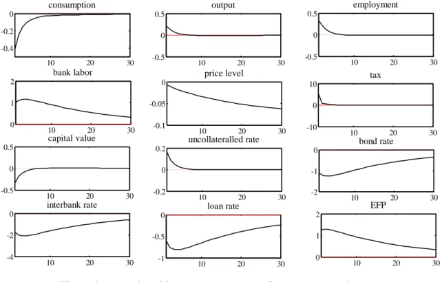
5.1.2 Large and rapid government expenditure

While the more persistent policy can successfully help the economy recover, most economists urge the

10 20 30 -0.4 -0.2 0 consumption 10 20 30 -0.5 0 0.5 employment 10 20 30 0 1 2 bank labor 10 20 30 -0.1 -0.05 0 price level 10 20 30 -10 0 10 tax 10 20 30 -0.5 0 0.5 capital value 10 20 30 -0.2 0 0.2 uncollateralled rate 10 20 30 -2 -1 0 bond rate 10 20 30 -4 -2 0 interbank rate 10 20 30 -1 -0.5 0 loan rate 10 20 30 0 1 2 EFP 10 20 30 -0.5 0 0.5 output

Fig. 6: large and rapid government expenditure:D_g 3 and _g 0.6.

response to the financial crisis when there is no room for further interest rate decreases, the

economy has run into recessions for more than 4 quarters, consumption and investment have fallen

significantly, and there seem to be no signs for the private sector to recover on its own accord.

Therefore, we propose another large and rapid government expenditure by assuming that D_g  and 3 0.6

g

  , which can generate a similar price level path to that under the previous policy. With the low persistence, the 3% increase in government expenditure in response to a 1% financial shock will die out

in 10 quarters approximately. Fig. 6 shows that this policy can stimulate the production immediately to

0.2%, but declines quickly with the less persistent spending. The fast adjustment speed also applies to

other variables. While the large government expenditure causes drastic drops in consumption and

investment initially, they rise back to the normal level in 5 quarters. Similarly, the tax increases greatly

at the beginning, but falls down and remains at the steady-state level after 4 quarters. Interest rates, on

the other hand, do not vary much with policies.

The quick recovery of the economy, 5 quarters before the government expenditure expires, provides

handle the drastic drop in consumption in the early period, without being adversely affected by the

current and future inflationary pressure, this enormous aggregate demand stimulus can help the private

sector to accumulate enough income and capital to restore the credit market as well as the economy to

its normal level before the crisis hit. Compared with the persistent but relatively small fiscal policy, this

policy would be more desirable as people wish to avoid the recession sustaining.

5.2 Monetary policy

Since the monetary policy can be easily implemented, it is usually the first step that the government

will take in response to the financial crisis. While the interest rate rule does not seem to be effective,

control over the base money is also exercised. This finding follows along the same lines as the

development of US policies after the outbreak of the financial crisis. While the Fed has consecutively

cut the Fed fund rate target from 5.25% to 0.25% within 5 quarters, there do not seem to be any signs

of a recovery. In March 2009, the chairman of the Fed, Ben Bernanke, announced that the Fed was

planning to purchase 300 billion in bonds from the markets. While this “quantitative easing” of the

environment seems to be needed for the economy, it is also accompanied by mounting worries over

high inflation after the recession ends. The analysis below may help explain the limited effects of the

interest rate rule, and the possible success of the quantitative easing strategy of the Fed.

5.2.1 Interest rate rule

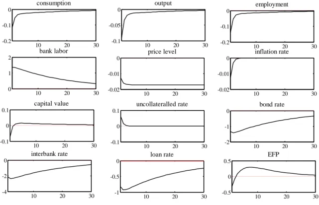
10 20 30 -0.2 -0.1 0 consumption 10 20 30 -0.1 -0.05 0 output 10 20 30 -0.2 -0.1 0 employment 10 20 30 0 1 2 bank labor 10 20 30 -0.02 -0.01 0 price level 10 20 30 -0.1 0 0.1 capital value 10 20 30 -0.1 0 0.1 uncollateralled rate 10 20 30 -2 -1 0 bond rate 10 20 30 -4 -2 0 interbank rate 10 20 30 -1 -0.5 0 loan rate 10 20 30 -0.5 0 0.5 EFP 10 20 30 -0.02 -0.01 0 inflation rate

Fig. 7: interest rate rule under a persistent financial shock: D_R  1, _k 0.95.

collateral effectiveness, and so D_R   . To characterize the persistent interest rate cut in 1

reaction to the prolonged crisis, the persistence of the interbank rate, ₃0.95, is specified. However, compared with Fig. 4, the interest rate cut does not result in much difference under the interest rate

smoothing rule, but causes larger declines in consumption and output as well as slight rises in interest

rates. The interest rate increases lower the discounted value of the marginal product of capital and thus

reduce the value of capital, compared with Fig. 4. The decline in investment worsens the downturn in

output and consumption.

This peculiar result may be caused by the relative magnitude of the interest rate rule’s responses to

the past interest rate and current inflation and output gap. While the 1% cut in the interest rate is not

large enough, the interest rate responds more to the current output gap and inflation rate. Because the

output rebounds to the normal level in only two quarters, the zero output gap prevents further interest

rate cuts. This result is quite robust even under an unrealistic 5% quarterly cut in the interest rate to the

shocks or inflation targeting rule with the assumption that ₁10 and ₂  . The calibrations of the 0 same policies under the

10 20 30 -0.5 0 0.5 consumption 10 20 30 0 0.2 0.4 output 10 20 30 0 0.5 employment 10 20 30 0 1 2 bank labor 10 20 30 0 0.05 0.1 inflation rate 10 20 30 0 0.5 capital value 10 20 30 -0.4 -0.2 0 uncollateralled rate 10 20 30 -4 -2 0 bond rate 10 20 30 0 2 4 EFP 10 20 30 -2 -1 0 loan rate 10 20 30 -4 -2 0 interbank rate 10 20 30 0 0.05 0.1 price level

Fig. 8: interest rate rule under less persistent financial shocks: D_R 1, k 0.7.

shock to the monitoring in the banking sector also generate the same results.

The crucial determinant seems to be the persistence of the shocks. If the persistence of the shock is

lowered to 0.7, instead of 0.95 as in previous cases, a 1% interest rate cut is enough to help the

economy recover regardless of whether it is interest rate smoothing, as shown in Fig. 8. Both

consumption and output rise slightly above the normal level, accompanied by an increase in investment.

This implies that the interest rate rule is not effective unless the credit market efficiency is quickly

restored, which in turn depends on the confidence of the banking sector in the production of loans. In

Fig. 7, we can see that although the banking sector hires more people to monitor the loan making and

the value of the capital goods increases, lower consumption implies that the outstanding loans remain at

a low level. The lower interest rate is not able to stimulate the banking employment or restore the

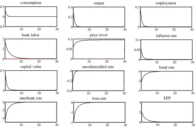
10 20 30 0 0.5 consumption 10 20 30 0 0.5 output 10 20 30 0 0.5 1 employment 10 20 30 0 0.5 1 bank labor 10 20 30 0 5 10 price level 10 20 30 0 0.5 1 capital value 10 20 30 0 0.5 1 uncollateralled rate 10 20 30 -0.5 0 0.5 bond rate 10 20 30 -2 0 2 interbank rate 10 20 30 -1 0 1 loan rate 10 20 30 0 1 2 EFP 10 20 30 0 0.5 1 inflation rate

Fig. 9: expansionary high-powered money: Dm 1.

rapidly recover. Therefore, the effectiveness of the interest rate rule strongly relies on the

reestablishment of the credit market is crucial for the economy to recover but not the other way round.

5.2.2 Expansionary monetary base

While the interest rate rule does not seem to be effective in the face of the crisis, the expansionary base

money seems to work much better. With the persistence of the high-powered money growth equaling

0.9 and responding to a 1% financial shock by a 1% increase in the growth rate of the monetary base,

Fig. 9 shows that the consumption and output can grow without experiencing the initial recession. The

1% increase in the base money will cause the interbank interest rate to fall by 1.14% in each quarter,

which is equivalent to 4.8% per annum. This decline does not seem to be unrealistic because the Fed

has lowered the Federal funds rate by 5% within just one year.17 The essential reason for the

effectiveness of the monetary expansion is the quantitative easing environment. While a larger

high-powered money growth induces a greater demand for consumption followed by higher deposit and

17

loan demand, the interest rates are lowered. A lower interest rate stimulates investments and the capital

stock, and is helpful in restoring the quantity of loans to a higher level.

In particular, from the balance sheet of the bank, H  , we can see that the bank reserves rise L D

with the expansion in high-powered money. Deposits are increased accordingly which can facilitate

consumption. This mechanism is absent from the conventional literature on monetary policy, which

neglects the banking sector, as well as from the studies on credit channels without considering money.

This channel is also absent in an economy with an interest rate rule which crucially depends on the

interest rate elasticity of consumption and investments.

6 Conclusion

This paper investigates quantitatively the macroeconomic implications of monetary and fiscal policies

under the current financial crisis based on the model in GM (2007). By using the DSGE model with the

banking sector, we can successfully characterize the financial crisis that was initiated in the credit

markets in terms of the shock to the loan production of banks and see how the shock impacts other

sectors within the economy. With money and banking, this model allows for the endogenous

determination of various interest rates and the EFP.

The effects of policies are examined quantitatively by means of calibrations based on US data where

the crisis started. The calibration results show that expansionary government expenditure can

successfully help the economy recover, but the timing and size of the policy’s implementation may

matter. When characterized by a 3% increase in government spending in response to a 1% shock to the

effectiveness of collateral with an AR(1) coefficient of 0.6, this policy will enable the economy to

crowding-out effect of fiscal policy due to rising interest rates will be attenuated. Therefore, a model

without distinct interest rates may overstate the crowding-out effects and the effects of the fiscal policy

may be stronger than was thought. While the credit channel literature focuses on the examination of

monetary policies, the implications of credit channels for fiscal policy have not been noted before.

The effects of monetary policy also strongly rely on the way the policy is applied. A 1% expansion in

the growth rate of base money in response to a unit shock to the effective collateral can successfully

stimulate the economic recovery. The increase in the monetary base can raise the demand for

consumption as well as deposits, thereby boosting the economic growth. However, with the high

persistence of the financial shock of 0.9, as in all other cases, a 4% p.a. interbank rate reduction by the

Fed will fail to pull the economy out of the recession, no matter how persistent the interest rate rule is

or how large the initial cut is (interest rate smoothing or inflation targeting). It will only be effective if

the financial shock is less persistent. That is, the effectiveness of the collateral needs to be restored

soon and thus the banking sector will be able or will be willing to provide enough loans for

consumption. This finding coincides with the fading effects of the interest rate rule since the financial

crisis broke out which has led to an emphasis on “quantitative easing” policy or massive government

spending. It shows that it is the effectiveness of the interest rate relies on the credit market restoration,

but not the other way round.

However, the policies in this model are relatively simple: the government expenditure focuses on

goods without contributing to productivity or consumption directly in the economy. There will be

differences if the emphasis is on productive spending or consumables. The way to finance the

government expenditure also matters. Whether the funds for the spending are raised by issuing bonds,

money or by taxes will result in different interest rate movements and the EFP, and these will have

References

Bernanke, B. S. and A. S. Blinder (1988) “Credit, Money and Aggregate Demand” American Economic Review,

78(2), 435-439.

Bernanke, B. S. and M. Gertler (1989) “Agency Costs, Net Worth, and Business Fluctuations” American

Economic Review, 79, 14-31.

Bernanke, B. S. and M. Gertler (1995) “Inside the Black Box: The Credit Channel of Monetary Policy Transmission” Journal of Economic Perspectives, 9, 27-48.

Bernanke, B., Gertler, M. and Gilchrist, S. (1998) “The Financial Accelerator in a Quantitative Business Cycle Framework” NBER Working Papers, No.6455

Carlstrom, C. T. and T. S. Fuerst (1997) “Agency Costs, Net Worth, and Business Fluctuations: a Computable General Equilibrium Analysis” American Economic Review, 87(5), 893-910.

Clarida, R., J. Galí and M. Gertler (1999) “The Science of Monetary Policy: A New Keynesian Perspective”

Journal of Economic Literature, 37, 1661-1707.

Clarida, R., J. Galí and M. Gertler (2000) “Monetary Policy Rules and Macroeconomic Stability: Evidence and Some Theory” Quarterly Journal of Economics, 105(1), 147-180.

Clarida, R., J. Galí and M. Gertler (2002) “A Simple Framework for International Monetary Policy Analysis”

Journal of Monetary Economics, 49(5), 879-904.

Cooley T. and R. Marimon (2004) “Aggregate Consequences of Limited Contract Enforceability” Journal

of Political Economy, 112, 817-847.

Edwards, S. and C. A. Végh. (1997) “Banks and Macroeconomic Disturbances under Predetermined Exchange Rates” Journal of Monetary Economics, 40, 239-278.

Goodfriend, M. and McCallum B. T. (2007) “Banking and Interest Rate in Monetary Policy Analysis: A Quantitative Exploration” Journal of Monetary Economics, 54, 1480-1507.

Kocherlakota, N. (2000) “Creating Business Cycles through Credit Constraints” Federal Reserve Bank of

Minneapolis Quarterly Review, 24(3), 2-10.

Kollmann, R. (2002) “Monetary Policy Rules in the Open Economy: Effects on Welfare and Business Cycles”

Journal of Monetary Economics, 49, 989-1015.

Schmitt-Grohé, S. and Martín Uribe (2002) “Optimal Fiscal and Monetary Policy Under Sticky Prices” NBER

Working Paper No. 9220

Sutherland, A. 2006. “The expenditure switching effect, welfare and monetary policy in a small open economy,” Journal of Economic Dynamics and Control, vol. 30, no. 7, pp. 1159~1182.

國科會補助專題研究計畫成果報告自評表

請就研究內容與原計畫相符程度、達成預期目標情況、研究成果之學術或應用價

值（簡要敘述成果所代表之意義、價值、影響或進一步發展之可能性）

、是否適

合在學術期刊發表或申請專利、主要發現或其他有關價值等，作一綜合評估。

1. 請就研究內容與原計畫相符程度、達成預期目標情況作一綜合評估



達成目標

□ 未達成目標（請說明，以 100 字為限）

□ 實驗失敗

□ 因故實驗中斷

□ 其他原因

說明：

2. 研究成果在學術期刊發表或申請專利等情形：

論文：□已發表



未發表之文稿 □撰寫中 □無

專利：□已獲得 □申請中 □無

技轉：□已技轉 □洽談中 □無

其他：（以 100 字為限）

本研究主題＂macroeconomic implications of policies under financial crisis＂ 一文已刊登於「世紀初金融風暴學術研討會」會議論文集中，並已 準備投稿學術期刊。相關研究 “Implications of Economic Openness for Financial Crisis” 已發表於社會科學論叢中( 第四卷第一期, 51-74 頁)。

3. 請依學術成就、技術創新、社會影響等方面，評估研究成果之學術或應用價

值（簡要敘述成果所代表之意義、價值、影響或進一步發展之可能性）（以

500 字為限）

本研究是在一包括金融中介機構的動態隨機一般均衡模型 (DSGE) 下探討金融部門所造 成的金融危機對於總體經濟的影響，以及貨幣政策與財政政策在這樣的金融衝擊下對於促 進總體經濟復甦的有效性。研究的結果發現，財政政策與量化寬鬆的貨幣政策是有效的， 但降息是無效的。此一研究，可以幫助我們瞭解金融危機對於總體經濟的衝擊，以及金融 風暴下，較為適當的政策措施。於學術面，此一模型可以更進一步幫助我們瞭解貨幣政策 的傳遞效果；於政策面，我們可以更清楚，政府應採取什麼樣的措施來因應金融風暴，協 助總體經濟的復甦。 本人並已將此研究延伸到小型開放經濟體系的架構下來探討金融風暴對於匯率，乃至總體 經濟的影響，亦藉此模型來探討台灣最適的貨幣政策。本次次級房貸風暴發生之後，國際 間對於金融中介機構與貨幣政策的研究於質與量上皆有大幅度的成長，因此，包含了金融 中介機構的 DSGE 模型在未來具有相當大的發展潛力。