不均勻外力作用於層狀半空間內之解析解

行政院國家科學委員會專題研究計畫 期末報告

不均勻外力作用於層狀半空間內之解析解

計 畫 類 別 ： 個別型 計 畫 編 號 ： NSC 101-2221-E-009-172- 執 行 期 間 ： 101 年 08 月 01 日至 102 年 09 月 30 日 執 行 單 位 ： 國立交通大學土木工程學系（所） 計 畫 主 持 人 ： 劉俊秀 計畫參與人員： 此計畫無其他參與人員 報 告 附 件 ： 出席國際會議研究心得報告及發表論文 公 開 資 訊 ： 本計畫可公開查詢

中 華 民 國 102 年 12 月 29 日

中 文 摘 要 ： 本研究主要是要求得埋在層狀半空間中任意分佈外力所造成 之地盤反應。目前能夠將外力加在層狀半空間內部的解，一 般是指 Green Function 的解，但 Green Function 為一集中 載重之解，因此會有奇異點(singularity)之現象。而本文是 以任意分佈載重模擬外力，因此不會有奇異點的現象。這對 目前利用邊界元素法(BEM)求地盤振動與基礎阻抗矩陣將會有 大幅度之改進。 本研究之求解過程中，將假設外力在徑向(r-方向)之分佈 為片段線性(piecewise linear)，在 θ-方向可分解成傅立 葉級數(Fourier Series)。此分佈外力可作用在任何深度。 然後可利用主持人過去所發展之方法直接求圓柱座標系統中 之波動方程式之解，其最後之解將為一 Bessel Function 之 積分式。本文法最大之持點為外力作用位置之位移沒有奇異 的現象。 又由於載重片段線性,因此只要求得一小區域線性分析之 解,即可求得所有片段線性分佈之解。本研究將漸漸縮小分佈 載重面積,以觀察其應力的集中性,及其對位移的影響。 中文關鍵詞： Wave Propagation, Analytic Solution, Green Function 英 文 摘 要 ： The paper is to deal with the problem of the response

of stratified half-space subjected to an arbitrary distributed loading on an axial symmetric area buried in stratified half-space. Except boundary element method, the response to a force buried in a

stratified half-space is rarely dealt with. However, Green function employed in boundary element method will creat singularity situation at the location of source point. The presented method can avoid the singularity situation, since the external loading is not a concentrated load and is arbitrarily

distributed over an axial symmetric area buried in stratified half-space.

In the process of the solution, the arbitrarily distributed loading can be decomposed into a Fourier Series in θ-direction and piecewise linear

distribution in r-direction is assumed for each Fourier component. Then the wave equations in

cylindrical coordinates are directly solved using the technique developed by the author. The solution will be an integral of Bessel function with respect to

wave number. The advantage of the method will be that singularity problem can be avoided.

Since the distributed loading is piecewise linear, one just need to solve the problem for a triangular distribution on an axial symmetric area and then sums up all the solution for all the triangular

distribution .This summation will be the solution for arbitrary distributed loading. Some numerical results for shrinking the distributed area will be given to show the concentrated effect of the distributed loading.

行政院國家科學委員會補助專題研究計畫成果報告

（□期中進度報告/



期末報告）

不均勻外力作用於層狀半空間內之解析解

計畫類別：



個別型計畫 □整合型計畫

計畫編號：NSC 101－2221－E－009－172

執行期間： 101 年 8 月 1 日至 102 年 9 月 30 日

執行機構及系所：

國立交通大學土木工程學系（所）

計畫主持人：劉俊秀

共同主持人：

計畫參與人員：

本計畫除繳交成果報告外，另含下列出國報告，共 _1_ 份：

□執行國際合作與移地研究心得報告



出席國際學術會議心得報告

期末報告處理方式：

1. 公開方式：



非列管計畫亦不具下列情形，立即公開查詢

□涉及專利或其他智慧財產權，□一年□二年後可公開查詢

2.「本研究」是否已有嚴重損及公共利益之發現：



否 □是

3.「本報告」是否建議提供政府單位施政參考



否 □是， （請列舉提

供之單位；本會不經審議，依勾選逕予轉送）

中 華 民 國 102 年 12 月 29 日

國科會補助專題研究計畫成果報告自評表

請就研究內容與原計畫相符程度、達成預期目標情況、研究成果之學術或應用價

值（簡要敘述成果所代表之意義、價值、影響或進一步發展之可能性）

、是否適

合在學術期刊發表或申請專利、主要發現（簡要敘述成果是否有嚴重損及公共利

益之發現）或其他有關價值等，作一綜合評估。

1. 請就研究內容與原計畫相符程度、達成預期目標情況作一綜合評估



達成目標

□ 未達成目標（請說明，以 100 字為限）

□ 實驗失敗

□ 因故實驗中斷

□ 其他原因

說明：

2. 研究成果在學術期刊發表或申請專利等情形：

論文：□已發表



未發表之文稿 □撰寫中 □無

專利：□已獲得 □申請中 □無

技轉：□已技轉 □洽談中 □無

其他：

（以 100 字為限）

投稿 Journal of Earthquake Engineering and Structure Dynamic

3. 請依學術成就、技術創新、社會影響等方面，評估研究成果之學術或應用價

值（簡要敘述成果所代表之意義、價值、影響或進一步發展之可能性）

，如已

有嚴重損及公共利益之發現，請簡述可能損及之相關程度（以 500 字為限）

本研究主要突破為求得小面積內分佈載重之解析解,與 Green function 相較,

本研究之解沒有奇異(singularity)值問題。

中文摘要。

關鍵詞:Wave Propagation, Analytic Solution, Green Function

本研究主要是要求得埋在層狀半空間中任意分佈外力所造成之地盤反應。目 前能夠將外力加在層狀半空間內部的解，一般是指Green Function的解，但Green Function 為一集中載重之解，因此會有奇異點(singularity)之現象。而本文是以任 意分佈載重模擬外力，因此不會有奇異點的現象。這對目前利用邊界元素法(BEM) 求地盤振動與基礎阻抗矩陣將會有大幅度之改進。 本研究之求解過程中，將假設外力在徑向(r-方向)之分佈為片段線性(piecewise linear)，在θ-方向可分解成傅立葉級數(Fourier Series)。此分佈外力可作用在任何 深度。然後可利用主持人過去所發展之方法直接求圓柱座標系統中之波動方程式 之解，其最後之解將為一Bessel Function 之積分式。本文法最大之持點為外力作 用位置之位移沒有奇異的現象。 又由於載重片段線性,因此只要求得一小區域線性分析之解,即可求得所有片 段線性分佈之解。本研究將漸漸縮小分佈載重面積,以觀察其應力的集中性,及其 對位移的影響。

Abstract

Keyword: Wave Propagation, Analytic Solution, Green Function

The paper is to deal with the problem of the response of stratified half-space subjected to an arbitrary distributed loading on an axial symmetric area buried in stratified half-space. Except boundary element method, the response to a force buried in a stratified half-space is rarely dealt with. However, Green function employed in boundary element method will creat singularity situation at the location of source point. The presented method can avoid the singularity situation, since the external loading is not a concentrated load and is arbitrarily distributed over an axial symmetric area buried in stratified half-space.

In the process of the solution, the arbitrarily distributed loading can be decomposed into a Fourier Series in θ-direction and piecewise linear distribution in r-direction is assumed for each Fourier component. Then the wave equations in cylindrical coordinates are directly solved using the technique developed by the author. The solution will be an integral of Bessel function with respect to wave number. The advantage of the method will be that singularity problem can be avoided.

Since the distributed loading is piecewise linear, one just need to solve the problem for a triangular distribution on an axial symmetric area and then sums up all the solution for all the triangular distribution .This summation will be the solution for arbitrary distributed loading. Some numerical results for shrinking the distributed area will be given to show the concentrated effect of the distributed loading.

Introduction

Ground vibration due to near-by sources has been paid attention to over past several decades. Especially, for the sensitive facility and high-tech productions equipment, this vibrations is annoying. Therefore, how to predict the vibrations become an important subject. Wood and Jedele [1] have collected some observed data and deduced them into a simple formula expressing attenuation phenomenon of ground vibrations in term of soil damping and distance between source and

observation locations. From more theoretical aspects, Sheng et al. [2] and Krylou [3] have employed Euler beam theory to model whole track including sleepers and ballast and then to solve the problem of moving train. Kaynia et al.[4] have proposed a more sophisticated analysis model, which takes dynamic interaction into account, to evaluate ground vibration induced by passing trains. Moreover, Karlstrom [5] has employed a refined semi-analytic model to investigate the effect on ground vibration due to accelerating train.

Most of the above analysis model, finite element or boundary element methods are used to model half-space medium or layered half-space medium. Regarding analytical approach to evaluate ground vibration due to a specific source, Apsel and Ruco [6] have calculated the vibrations at the locations on half-space medium due to a point source (Green’s Function). Vostroukhov [7] et al. have employed integral transform method to obtain ground vibration in layered half-space due to a buried uniform load at a circular area.

Also, Kausel and Peer [8] has employ layer elements to obtain Green function for layered medium. Green function has been the fundamental solution for the boundary element method. However, the singularity situation occurs at the location of source point. The major task of boundary element method is to deal with the singularity problem. The paper is trying to obtain the solution for distributing the point

(concentrated) load to a small area. Therefore, the singularity problem will disappears. In the solution process, the distributed loading on an axial symmetric area can be decomposed into an infinite series of Fourier components with respect to azimuth. For each Fourier components, triangular distribution in r -direction is assumed.

To solve the problem mathematically, the whole layered half-space medium is divided into two domains (upper and lower domains), the upper domain is the domain above the level where the external loading is applied, and the other one is the lower domains which is below the level. For each domain, the technique of decomposing the loading, which is developed by Liou [9], is employed. The decomposed loading will automatically match the forms of boundary values of general solutions of three dimensional wave equations in cylindrical coordinates for the layered stratum. Then,

the boundary conditions of free surface , attenuation phenomenon, and the continuity conditions of displacement and stress components at the interface of the two domains (above and below the level) are imposed to obtain the solution .

The analytical expression for vibration at a specific location in a layered medium will end up with a form of semi-infinite intergration with respect to wave number

k

, and Rayleigh singular pole existing in the integration path if there is no material damping in the medium. However, if material damping is always assigned in the medium, the singular pole will move away from intergration path. And, from the decaying nature of the integrand with respect to wave number

k

as proven in Liou’s work [10], the vibration can be calculated by integration only up to a certain upper limit

k

_uwithout losing accuracy.

The numerical results for the cases of equal magnitude of total loading with different distribution areas will be compared each other. This will show the

phenomenon of variation of stress and displacement components around the different distribution areas of the total loading. The solution should be close to Green function solution as the distribution area getting smaller. However, no singularity situation like that in Green function solution at source point will occur in the presented solution.

Analytical Solutions For Dynamic Loadings In Layered Medium

The general solution of the differential equations for wave propagation in

cylindrical coordinates is independently found for each layer in layered medium. The displacement and stress continuity conditions at the horizontal interfaces in layered system are then imposed for further expressing the displacement and stress fields in terms of the prescribed dynamic loadings. The total system of prescribed dynamic loadings applied in layered half-space is shown in Figs.1. In Fig.1(a), the shaded area is the locations where dynamic loading is applied. Fig.1(b) shows the distribution of the dynamic load in r-direction for each Fourier component. The prescribed dynamic loadings on axially symmetric area can be expressed in cylindrical coordinates in terms of Fourier components with respect to azimuth as follows :

t i 0 n n z n zz n rz t i z zz rz e ) n sin( ) n cos( ) r ( ) n sin( ) n cos( ) r ( ) n sin( ) n cos( ) r ( e ) , r ( ) , r ( ) , r (                   



                                                  

r

1



r



r

2

,

z



h

i (1)

where superscript

n

denotes th



2 r

r₁ ₂ .

Since the time variation iωt

e appears on both sides of the equation, it will be omitted hereinafter. For the cases of dynamic loadings applied at arbitrary area, the loading can be expressed by the summation of several axial symmetric areas in Eq.(1) .

Since the external load is applied at level i in Fig1(a), the domain is divided into two domains. One is the domain above level i and the other is the domain below level

i. One can consider the domain below level i first. As show in Fig.1(a), the general

differential equations for wave propagation in a particular layer j with harmonic excitation can be obtained using the technique separating the dilatational wave from the rotational wave . And the technique of separation of variables is employed to solve the independent differential equations for the dilatational wave and the rotational wave. After combining the solutions for the dilatational and the rotational waves, the general solution of the differential equations of wave propagation for n Fourier th

component can be expressed in the matrix form as follows :

r z θ cosnθ cosnθ u (r,z) 0 0 sinnθ sinnθ cosnθ cosnθ u (r,z) = 0 0 sinnθ sinnθ -sinnθ -sinnθ u (r,z) 0 0 cosnθ cosnθ                      _{ }  _{ }   _{  }                 _{ } _{ }    _{ } _{ }            1 Jκ eA (2) or 1 Lu = LJκ eA where n n n n n J (kr) 0 (n/r)J (kr) = 0 kJ (kr) 0 (n/r)J (kr) 0 J (kr)             J (3)

matrix κ1 is defined by Eq. (A-1) in Appendix,

vector A= ( A , B , C , A , B , C )1 1 1 2 2 2 T is unknown coefficient vector determined

from the boundary conditions at the upper and the lower interfaces of the layer, 6 6

diagonal matrix -v zj -v zj -v zj v zj v zj v zj

= diag( e , e  , e  , e , e , e ),

2 2 2 2 2 2

j pj j gj

ν = k - (ω /c ) , ν = k - (ω /c ),

pj

c

and

c

_gj are compressional and shear wave velocities respectively in the layer ( jth layer),

k

is wave number in horizontal direction, J (kr)_n is first kind of Bessel function of order n, and J (kr) = [dJ (kr)/dr]_n _n .

The stress field in the layer can be obtained by differentiating the displacement field of Eq.(2) with respect to the corresponding variables r , z and θ , and then multiplying it with constitutive matrix of elasticity. The stress components on horizontal plane, with the azimuthal variation of matrix L (representing symmetric and antisymmetric Fourier components with respect to θ=0 ) in Eq.(2) factored out, can then be expressed as follows :

rz zz θz τ (r,z) t = σ (r, z) = τ (r,z)           2 Jκ eA (4)

where matrix κ₂ is defined by Eq.(A-2) in Appendix.

Since the unknown coefficients in vector A are determined from the boundary conditions of the layer, the displacement and the stress fields of Eqs.(2) and (4) can be expressed in terms of the unknown displacement and stress components at the lower interface of the layer [9,11]. Moreover, the displacement and stress components at the upper interface can be combined together and written in terms of the displacement and stress components at the lower interface as follows [9,11]:

j 1 j 1 j Ea E Y Y _   (5) where 6 6 matrix Ediag



J J,



in which Bessel matrix J is shown in Eq.(3), transfer matrix a = κej -1(d )_j κ-1 is defined by Eq.(A-3) in Appendix in which matrix

   T1 T2 T κ = κ , κ , diagonal matrix j j z=d (d ) = |

e e in which djis the thickness of the

layer, and Yj1 and Yj are the unknown displacement-stress vectors at the upper

and the lower interfaces of the layer, respectively.

Consider the total lower domain shown in Fig.1. For a given layer in the system, Eq.(5) shows that the displacement-stress vector at the upper interface can be

expressed in terms of the displacement –stress vector at the lower interface. Therefore, by imposing the displacement and stress continuity conditions at the horizontal

interfaces from the first top layer down to the half-space layer, one can obtain the displacement-stress vector at the surface of the total system in terms of the displacement-stress vector at the surface of the half-space layer as expressed by Eq.(6). M 1 M 1 ME Y ETE Y a a Ea Y_i  _{i1 i2}    (6) Consider the half-space layer in Fig.1 alone. The general solutions of differential equations of wave propagation and the stress field in the half-space layer are similar to Eqs.(2) and (4) respectively except that upward propagating reflection waves do not exist. The displacement-stress vector at the surface of the half-space layer can then be written as   _{ }     M M M u Y = = Eκ A t (7)

where matrix κ = κ , κ _ ₁T ₂T_T in which submatrices κ1 and κ2 are defined by

Eqs(A-1a) and (A-2a) in Appendix respectively, and A= (A ,B ,C )_{1 1 1} T is unknown coefficient vector determined from the boundary conditions at the surface of the half-space layer.

Substituting Y_Min Eq.(7) into Eq.(6) , Eq.(6) can be written as

A κ κ T T T T J 0 0 J t u Y 2 1 22 21 12 11 i i i                              ₍₈₎

where T11 ~ T22 are submatrices of matrix T in Eq.(6). After some matrix

manipulations of eliminating the unknown vector A , one can obtain the 

displacement vector

u

_i in terms of the stress vector

t

_i .



11 1 12 2



21 1 22 2



1 1 i 1 i i J T κ T κ T κ T κ J t JQJ t u            (9) i 1 1 i JQ J u t    (9a) If the layered medium has a rigid lower boundary, then uM = 0 in YM of Eq.(6).

This leads to Q = T T_{12 22}-1 for Eq.(9).

Now, consider the upper domain(above level i ). The derivation is similar to the derivation for lower domain (below level i) above (Eqs.4-9). But the boundary condition at is traction free for free surface.

Therefore, the displacement-stress vector at free surface can be expressed as

i 1 i 1 1 i 1 1 0 Ea a E Y ETE Y Y        ₍₁₀₎ or































































 i i 22 21 12 11 0 0

t

u

J

0

0

J

T

T

T

T

J

0

0

J

t

u

1 (10a) Applying the boundary condition of free surface t0=0, one can obtain

i 1 21 1 22 i JT T J u t    (11) i 1 22 1 21 i

J

T

T

J

t

u





  _(11a)

By comparing

t

iin Eq.(11) and

t

itin Eq.(9), one can say that t - i t must be equal i to n component of external load in Eq.(1) due to the stress continuity. This can be th

expressed as n i i

t

t

t





(12) where tn 



τrzn(r), σzzn(r), τnz(r)



T in Eq.(1)

As shown in Fig.1(b), the external loadings are assumed to be triangularly distributed. Thus, the loading distribution in r-direction can be expressed as follow;

h(r)s

τ

and

,

h(r)q

σ

h(r)p

τ

n θz n zz n rz



,





(13) where







































otherwise

0

r

r

r

if

ε

r

r

1

r

r

r

if

ε

r

r

1

h(r)

0 _{0 0} 0 0 0





(13a)

,

2 r r

r₀  1 2 _,

p

_,

q

and

s

are intensities of there kinds of distributed loadings. The technique developed by Liou [9, 11] is employed to decompose the loadings in Eqs.(13). And after some mathematical manipulations as shown in Liou’s work[9], one can obtain the following equation.





                                                 0 1 n 1 n 1 n 1 n n 1 n 1 n 1 n 1 n 0 n z n zz n rz n dk dk s q p D D 0 D D 0 D 0 D D 0 D D JDP J τ     (14) where J ( k r )h ( r ) d r 2 r D 2 r 1 r n 1 1 n 



 D rJ ( k r )h ( r ) d r 2 r 1 r n n 



(14a) and ₂ J (kr)h(r)dr r D r2 1 r n 1 1 n 





Now, one can employed Eq.(12) by substituting Eqs.(9a), (11) and (14) into Eq.(12) ,one can obtain









T κ T κ T κ T κ T T



DPdk J u 1 0 21 1 -22 1 -2 12 1 11 2 22 1 21 i  



        ₍₁₅₎

After displacement vector ui 



ur, uz, uθ



T has been obtained, one can employ

Eqs.(9a) and (11) to calculated the stress components ti 



τrz, σzz, τθz



T and





T

i

t  τ_rz, σ_zz, τ_θz at level i for lower and upper domains in Fig.(1), respectively .

Since the displacement vector u and stress vectors i tiand ti have been

obtained , the displacement components and stress components on every horizontal plane in both domains can be calculated by using the formula similar to Eqs.(10) or (6). These formula can be derived easily.

For the stress components on the vertical cylindrical surface, one can employed the equations derived in references 9 and 11.

                                           u u u z r z zz rz r rz rr 1 2 1 1J J J J ₍₁₆₎ where                0 0 0 (kr) J r n 0 (kr) J 0 (kr) kJ 0 n n n 1 J _(16a)                                   _{ }       _{ }     (kr)) J 2 k r n r (kr) J G( 2 0 (kr) J r n (kr) J r n G 2 0 0 0 (kr) J r n (kr) J r n G 2 0 )) kr ( J r n r ) kr ( J ( G 2 n 2 2 2 n n 2 n n 2 n n 2 2 n 2 J _(16b)

matrix J is expressed in Eq.(3),

G

is shear modulus and u , r u , z u ,  rz, zz

 and



_z are the displacement and stress components at horizontal plane of the same locations where rr,



rzand



r are being calculated.

In Eq.(16b), one may observe that some elements in matrix J is infinite as r→0 2 for n=1. However, if the Bessel functions in the elements are expressed by

polynominal functions, one can conclude that the infinite terms will be cancelled out each other in the elements. This means that there is no infinite element in matrixJ2 for r=0.

Numerical Analysis

The solutions presented in the paper have been verified with Green function solution[10] for the case of distributed loading applied at free surface. To the cases of distributed loadings buried in layered half-space, two types of media have been chosen. One is a layer over rigid bedrock. The other is half-space. For the medium of

one layer over rigid bedrock, the nondimensional layer thickness _{Re( )}

h h Cs 2





 _=0.5,

of the layer. For the two types of media, the distributed loadings are buried at nondimensional depth of ) Re( h h i i Cs 2





 _{=0.15, Poisson ratio is 0.33, and hysteretic} damping ratio is 0.05. In order to investigate the concentration effect of the loadings, three distributed areas are selected. Referring to Fig.1(a), first case is

r

1 =0.125 and

2 r =0.375 (ε=0.125) in which ) Re( 2 r r 1 1 Cs





 _and ) Re( 2 r r 2 2 Cs    _{; second case is}

_r

₁

=0.2 andr2=0.3 (ε=0.05); third case is

r

1=0.225, r2=0.275 (ε=0.025). In order to

keep the magnitude of total load equal among the three cases, the

intensities are 1.0 for case 1 (ε=0.125) , 2.5 for case 2.5 (ε=0.05) and 5.0 for case 3 (ε=0.025). Figs.2 show the real and imaginary parts of stress component σzz

on the horizontal plane at hi=0.15 for the case of one layer system with symmetric

Fourier component n=0. The nondimensional depth hi=0.15 means the horizontal

plane is the interface where external loading is applied. In the figures, one can observe six curves representing the results at the surfaces of both upper and lower domains with ε=0.125, 0.05 and 0.025 respectively. From Fig.2(a), one can see that the differences between upper and lower domain surfaces only occurs at the locations where external distributed loading is applied, and the difference at r =0.25 are 5.0 for case of ε=0.025, 2.5 for ε=0.05 and 1.0 for ε=0.125. These 5.0, 2.5,and 1.0 are the highest intensities of distributed loads for the three cases, respectively. Referring to Fig.2(a), one can observe that stress component in the region, where external load is applied, is smaller for upper domain. Also, from Figs.2(a) and 2(b), one can observe the stress continuity at the interface of upper and lower domains. In Fig.2(b), one can also see that the imaginary part of the stress component is almost the same forr ≧0.4 for the three cases of ε=0.125, ε=0.05 and 0.0025 of both media. Figs.3 shows the stress component



_rz on the horizontal plane of hj=0.15 and for the case of

half-space with symmetric Fourier component n=1. From the figures, one can observe the similar phenomena to that of Figs.2. One just only has to note that the stress component must multiply cosθ, if the location is not on θ=0 axis. Figs.(4) show the displacement uθ for the cases of both one layer system and half-space withhj=0.15

and anti-symmetric Fourier component n=0 . From Fig.4(a), one can see that the maximum displacement occurs around the location where highest intensity of loading

is applied. This phynomenern can also be observe in Figs2.(a)and3(a). The displacement values are getting close to each other as

r

is farther away from the location where the distributed loading is applied for the three cases of ε=0.125, 0.05,and 0.025. Also, the difference between the results for the cases of one layer system and half-space is getting apparent as

r

become farther. Figs.5 show the displacement component u for the cases of both one-layer system and half-space _z

with hi=0.15 and symmetric Fourier component n=1. From Fig.5(a), one can see that

the displacement is getting closer for the case of one-layer system or half-space, if

r

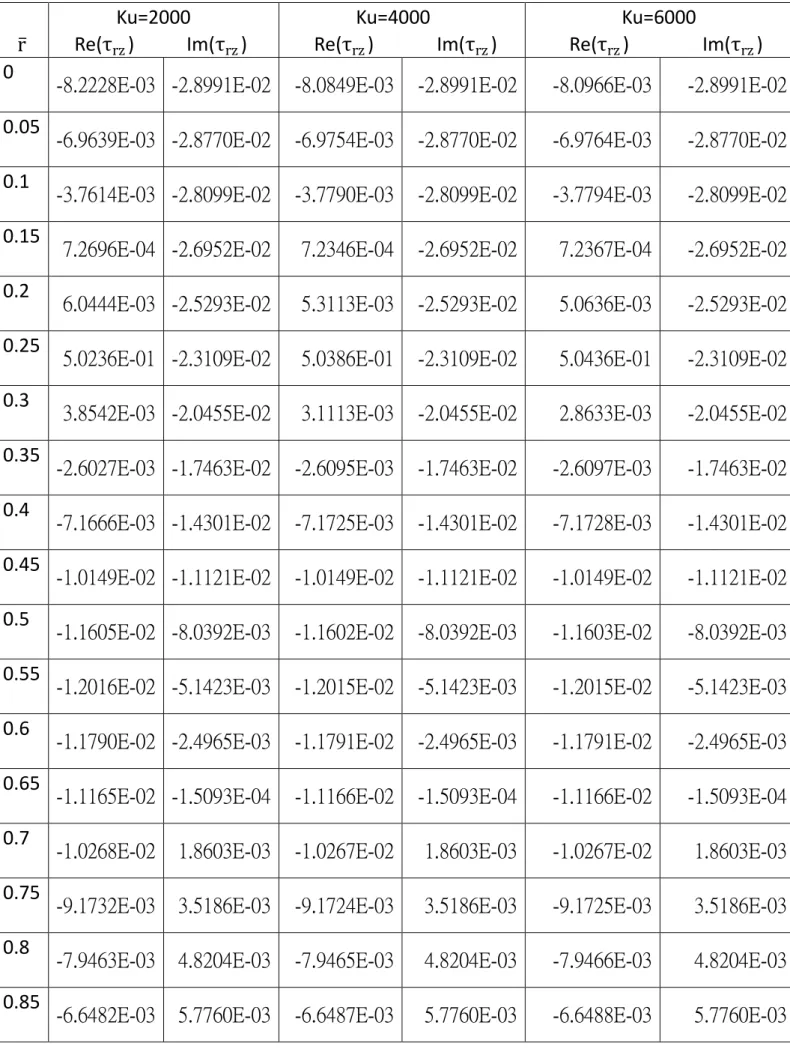
becomes farther. The difference among the cases of ε=0.125, 0.05 and 0.125 only occurs at region where external loading is applied. From Figs 2-5, one also can observe that the peak values is higher as the distributed loading is more concentrated. In order to know the effect of trunction of integrals in equations like Eq.(15), Table 1 shows the results of



rzfor the case of one-layer system with hi=0.15 and ε=0.05.

In the table, nondimensional wave number

k

_u is employed to replace the infinite integration limit (∞) in equations like Eq.(15). The nondimensional wave number is nondimemsionalized by shear wave velocity and frequency; i.e

k

_u=





2

kC

_s

. Table 1 only shows the results at surface of lower domain. From the table, one can observe that the results for

k

_u=2000, 4000 and 6000 are the same up to three figures. This means that

k

_u=2000 to replace infinite integration limit is good enough for

numerical calculations. Although the numerical results for displacement components are not shown, the precision is even much better. For example, in this case, the number of significant figures is five.

Concluding remarks

After thorough numerical investigations , the presented solution is very efficient in computation. The solutions presented in the paper can be easily employed to solve the problem of elastodynamic by fundamental solution method . The advantage of the presented solution is that no singularity situation could occur in the solution process .

The financial support of this research is provided by National Science Council of Taiwan through Contract no.NSC－101－2221－E－009－172

The support is appreciate.

Appendix

The matrix κ₁ in Eq. (2) can be expressed as follows :



 



1 1 1 κ = κ κ (A-1) where j j k -v 0 = -v k 0 0 0 1       _{ }     1 κ (A-1a) and j j k v 0 = v k 0 0 0 1             1 κ (A-1b)

The matrix κ₂ in Eq. (4) can be expressed as follows :



 



2 2 2 κ = κ κ (A-2) where j j 2 2 j j j β 2 2 j β j j j jj -2kG v G (2k - k ) 0 = G (2k - k ) -2kG v 0 0 0 -G v      _  _        2 κ (A-2a) and

j j 2 2 j j j β 2 2 j β j j j j 2kG v G (2k - k ) 0 = G (2k - k ) 2kG v 0 0 0 G v      _  _  _     2 κ (A-2b) in which j 2 2 β 2 gj ω k = c , j

G is shear modulus of jthlayer.

The transfer matrix aj in Eq. ( 5 ) can be expressed as follows :

      11 12 j 21 22 a a a = a a (A-3) where j j j j j j 2 2 2 β j 2 2 j β β 2 2 2 j β 2 2 j β β 2k k SH (CH - CH )+ CH (2k - k ) - 2v SH 0 v k k k SH 2k = -2v SH + (2k - k ) CH - (CH - CH ) 0 v k k 0 0 CH          _ _           _{  }   _{ } _     _       11 a (A-3a)     j j j j 2 j 2 2 j j β j β 2 j 2 2 j j β j β j j 1 SH -k v SH - k CH - CH 0 v G k G k k 1 SH = CH - CH v SH - k 0 v G k G k SH 0 0 -G v         _ _           _{  }   _{ } _     _  _     12 a (A-3b) j j j j j j j j j j 2 2 2 2 β j 2 2 j 2 2 2 β j β β β 2 2 2 ₂ β j 2 2 β j j 2 2 2 j β β β j j (2k - k ) -2kG -4k SH G v SH +_j (2k - k )(CH - CH ) 0 v k k k (2k - k ) 2kG SH 4k = (2k - k )(CH - CH ) G - v SH 0 v k k k 0 0 -G v SH   _    _ _    _{ }             _{ }   _{ }   _{ }         21 a (A-3c)

j j j j j j 2 2 2 j β 2 2 j β β 2 2 2 j β 2 2 j β β 2k k SH (CH - CH ) + CH 2v SH - (2k - k ) 0 v k k k SH 2k = 2v SH - (2k - k ) CH - (CH - CH ) 0 v k k 0 0 CH  _{ }     _{ } _           _{  }     _ _     _       22 a (A-3d)

in which SH = sinhν d_{j j}, SH = sinhν d j j, CH = coshν dj j, and CH = coshν d j j.

References

[1] R. D. Woods, P. J. Larry, “Energy-Attenuation Relationships from Construction Vibrations,” Proceedings of Vibration Problems in Geotechnical Engineering Convention, Detroit, Michigan(1985), 229-246.

[2] X. Sheng, C. J. C. Jones, M. Petyt, “Ground vibration generated by a load moving along a railway track ”, Journal of Sound and Vibration, 228(1) (1999), 129-156.

[3] V. V. Krylov, “Vibrational impact of high-speed trains. I. Effect of track dynamics. ”, Journal of the Acoustical Society of America, 100(5) (1996), 3121-3134.

[4] Amir M. Kaynic, Christian Madshus, Peter Zackrisson, “Ground vibration from high-speed train: prediction and countermeasure.”Journal of Geotechnical and Geoenvironmental Engineering , 126 (6) (2000), 0531-0573.

[5] Anders Karlstrom , “An analytical model for ground vibrations from accelerating trains” Journal of Sound and Vibration, 293 (2006), 587-598.

[6] R. J. Apsel, J. E. Luco, “On the Green’s functions for a layered half-space, partⅡ” Bulletin of Seismological Society of America 73 (4) (1983) 931-951.

of a stratified half-space subjected to a horizontal arbitrary buried uniform load appied at a circular area”Soil Dynamics and Earthquake Engineering 24 (2004) 449-459.

[8]Eduardo Kausel, and Ralf Peek, “Dynamic Loads In The Interior Of a Layered Stratum: An Explicit Solution ”Bulletin of the Seismological Society of America Vol.72 , No.5, (1982), 1459-1481

[9] G.-S. Liou, “Analytical solution for soil-structure interaction in layered media. ” J. of Earthquake Engineering. And Struct. Dynamics, 18(5), (1989)

,667-686

[10] G.-S. Liou,“Vibrations induced by harmonic loadings applied at circular rigid plate on half-space medium.”Journal of Sound and Vibration, 323 (1-2), (2009) 257-269.

[11] G.-S. Liou, I-L Chung. “Impedance matrices for circular foundation embedded in layered medium.”Soil Dyn Earthquake Eng, 29 (4), (2009), 677-692.

Table 1:Comparisons for different upper limits to replace infinite limit

r

Ku=2000

Re(τ

rz

) Im(τ

rz

)

Ku=4000

Re(τ

rz

) Im(τ

rz

)

Ku=6000

Re(τ

rz

) Im(τ

rz

)

0

-8.2228E-03 -2.8991E-02 -8.0849E-03 -2.8991E-02

-8.0966E-03

-2.8991E-02

0.05

-6.9639E-03 -2.8770E-02 -6.9754E-03 -2.8770E-02

-6.9764E-03

-2.8770E-02

0.1

-3.7614E-03 -2.8099E-02 -3.7790E-03 -2.8099E-02

-3.7794E-03

-2.8099E-02

0.15

_{7.2696E-04 -2.6952E-02}

_{7.2346E-04 -2.6952E-02}

_7.2367E-04

_-2.6952E-02

0.2

6.0444E-03 -2.5293E-02

5.3113E-03 -2.5293E-02

5.0636E-03

-2.5293E-02

0.25

5.0236E-01 -2.3109E-02

5.0386E-01 -2.3109E-02

5.0436E-01

-2.3109E-02

0.3

3.8542E-03 -2.0455E-02

3.1113E-03 -2.0455E-02

2.8633E-03

-2.0455E-02

0.35

-2.6027E-03 -1.7463E-02 -2.6095E-03 -1.7463E-02

-2.6097E-03

-1.7463E-02

0.4

_{-7.1666E-03 -1.4301E-02 -7.1725E-03 -1.4301E-02}

_-7.1728E-03

_-1.4301E-02

0.45

-1.0149E-02 -1.1121E-02 -1.0149E-02 -1.1121E-02

-1.0149E-02

-1.1121E-02

0.5

-1.1605E-02 -8.0392E-03 -1.1602E-02 -8.0392E-03

-1.1603E-02

-8.0392E-03

0.55

_{-1.2016E-02 -5.1423E-03 -1.2015E-02 -5.1423E-03}

_-1.2015E-02

_-5.1423E-03

0.6

-1.1790E-02 -2.4965E-03 -1.1791E-02 -2.4965E-03

-1.1791E-02

-2.4965E-03

0.65

-1.1165E-02 -1.5093E-04 -1.1166E-02 -1.5093E-04

-1.1166E-02

-1.5093E-04

0.7

-1.0268E-02 1.8603E-03 -1.0267E-02

1.8603E-03

-1.0267E-02

1.8603E-03

0.75

-9.1732E-03 3.5186E-03 -9.1724E-03

3.5186E-03

-9.1725E-03

3.5186E-03

0.8

_{-7.9463E-03 4.8204E-03 -7.9465E-03}

_4.8204E-03

_-7.9466E-03

_4.8204E-03

0.85

z 0 h_i z r_{1 r} 2 o 1 i j M Half-space

£n

_£cz

e

i£ st

£n

rz

e

i£ st £mzzei£ st

Figs.1:

total system of layered half-space and

triangular load distribution at depth h

_i

(a)

Figs.2: stress component σ

zz

for the case of one layer over rigid

bedrock,



0

.

15

i

h

and n=0

-3.0 -2.0 -1.0 0.0 1.0 2.0 3.0 0 0.1 0.2 0.3 0.4 0.5 0.6 0.7 0.8 0.9 ε=0.125 upper domain ε=0.05 upper domain ε=0.025 upper domain ε=0.125 lower domain ε=0.05 lower domain ε=0.025 lower domain -1.4 -1.2 -1.0 -0.8 -0.6 -0.4 -0.2 0.0 0.2 0 0.1 0.2 0.3 0.4 0.5 0.6 0.7 0.8 0.9 ε=0.125 upper domain ε=0.05 upper domain ε=0.025 upper domain ε=0.125 lower domain ε=0.05 lower domain ε=0.025 lower domain

Figs.3: stress component τ

rz

for the case of half-space,



0

.

15

i

h

and n=1

-3 -2 -1 0 1 2 3 0 0.1 0.2 0.3 0.4 0.5 0.6 0.7 0.8 0.9 ε=0.125 upper domain ε=0.05 upper domain ε=0.025 upper domain ε=0.125 lower domain ε=0.05 lower domain ε=0.025 lower domain -0.08 -0.07 -0.06 -0.05 -0.04 -0.03 -0.02 -0.01 0 0 0.1 0.2 0.3 0.4 0.5 0.6 0.7 0.8 0.9 ε=0.125 upper domain ε=0.05 upper domain ε=0.025 upper domain ε=0.125 lower domain ε=0.05 lower domain ε=0.025 lower domain

Figs.4: Displacement component u

θ

for the cases of one-layer

system and half-space,



0

.

15

i

h

and n=0

-0.1 -0.05 0 0.05 0.1 0.15 0.2 0 0.1 0.2 0.3 0.4 0.5 0.6 0.7 0.8 0.9 ε=0.125 h ̅=0.5 ε=0.05 h ̅=0.5 ε=0.025 h ̅=0.5 ε=0.125 halfspace ε=0.05 halfspace ε=0.025 halfspace -0.1 -0.08 -0.06 -0.04 -0.02 0 0.02 0.04 0 0.1 0.2 0.3 0.4 0.5 0.6 0.7 0.8 0.9 ε=0.125 h ̅=0.5 ε=0.05 h ̅=0.5 ε=0.025 h ̅=0.5 ε=0.125 halfspace ε=0.05 halfspace ε=0.025 halfspace

Figs.5: Displacement component u

z

for the cases of one-layer

system and half-space,



0

.

15

i

h

and n=1

-0.1 -0.05 0 0.05 0.1 0.15 0.2 0 0.1 0.2 0.3 0.4 0.5 0.6 0.7 0.8 0.9 ε=0.125 h ̅=0.5 ε=0.05 h ̅=0.5 ε=0.025 h ̅=0.5 ε=0.125 halfspace ε=0.05 halfspace ε=0.025 halfspace -0.15 -0.13 -0.11 -0.09 -0.07 -0.05 -0.03 -0.01 0.01 0.03 0 0.1 0.2 0.3 0.4 0.5 0.6 0.7 0.8 0.9 ε=0.125 h ̅=0.5 ε=0.05 h ̅=0.5 ε=0.025 h ̅=0.5 ε=0.125 halfspace ε=0.05 halfspace ε=0.025 halfspace

國科會補助專題研究計畫出席國際學術會議心得報告

日期：102 年 12 月 29 日

一、參加會議經過

本人於九月一日到達開普敦,當天下午報到。及聽一位 Keynote speaker 之演講。本人之 oral presentation 被安排在九月二日下午。全部論文之 oral presentation 發表的時間共三天(九月二 日至九月四月),同時有八箇平行 sessions,故論文發表超過五百篇。九月五日後本人自行在 Cape Town 旅行數天。

二、與會心得

本次會議超過 600 多個工程師、學者參與，其成員主要來自歐、美各國，來自台灣只有數人參與， 因此與各國學者互動良好。參加此次會議後，本人發現我們雖有國際知名的台北 101 大樓，但在 建築結構方面的會議卻很少參加。如此將會造成我們國內對國際建築結構的形式及其發展的概念 了解甚少，而國外之學者與工程師除了知道台北 101 大樓外，也甚少了解國內的發展情形，因此 類似此方面的會議，應鼓勵國內學者與工程師參加。

三、發表論文全文或摘要

計畫編號

NSC 101－2221－E－009－172

計畫名稱

不均勻外力作用於層狀半空間內之解析解

出國人員

姓名

劉俊秀

服務機構

及職稱

國立交通大學土木工程學系（所） 教授

會議時間

102 年 9 月 1 日至

102 年 9 月 4 日

會議地點

Cape Town, South Africa

會議名稱

(中文)

(英文) SEMC 2013 International Conference

發表題目

(中文)

1 INTRODUCTION

Due to urban development and economic necessi-ty, tall building becomes an solution for the con-centration of population. As the building is getting taller, the technique to withstand the horizontal loadings induced by earthquake and wind is more demanding. To resist the horizontal loading, many structural systems are available such as large-scale bracing, core, diagrid, outrigger, framed tube structures and others as explained by Ali and Moon(2007).

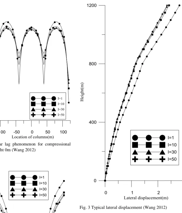
Among these structure forms, framed tube structure has the advantage of arranging all the re-sisting component at the perimeter of the building. This makes the components more efficient to re-sist the overturning moment caused by horizontal loading. The concept of tubular structure was first proposed by Khan and Amin (1973). However, the disadvantage of tubular structure is the shear-lag problem. The shear shear-lag will reduce the effi-ciency of the components . Therefore, bundle tub-ular structure is introduced as explained by Ali and Moon (2007) in order to relieve the problem of shear lag. Wang (2012) has presented the typi-cal shear lag phenomenon in Fig. 1 for a 3x3 bun-dle tubular structure with some modular tubes curtailed at the heights of 400 m and 800 m. In the figure, symbol I is relative moment of inertia of cross sections of spandrel beam. However, for the higher story, Singh and Nappal (1994) have shown that negative shear lag will occur. The typ-ical negative shear lag phenomenon is shown in Fig.2 for the 3x3 bundle tubular structure by Wang ( 2012 ). This means that the axial stress of

the interior column in the flange frame is larger than that of the exterior column. By observing Figs. 1 and 2,one can conclude that as the moment of inertia of cross section of spandrel beam ( I ) becomes larger, the effect of shear lag will be re-duced .As the effect of shear lag is diminishing, the tubular phenomenon becomes more apparent. This can be observed in Fig. 3. In the figure, the vanishing of shear lag effect, as seen in Figs.1 and 2, will make the horizontal stiffness of the building larger. This means the lateral displacement of the building subjected to horizontal loading is re-duced.

In order to mitigate the shear lag problem, a pyramid-like tubular structural form is suggested for tall buildings. The pyramid-like tubular struc-ture is defined as the tubular strucstruc-ture with gradu-ally reduced floor area through the height of floor. Since the floor area is reduced through the height, the periphery columns have to be inclined accord-ingly. The inclined columns can balance part of horizontal load directly. This could also mitigate the shear lag problem.

The paper will investigate the behavior of the pyramid-like tubular structure by changing the rel-ative stiffness of spandrel beams to periphery col-umn, and the effectiveness of the structure type for withstanding horizontal load. Also, the shear lag phenomenon for the structural type will be discussed. The analysis program SAP 2000 will be employed to model and analyze the structures. In the analysis model, only 3-D beam elements are used and rigid zone at beam-column joints is as-sumed.

Parametric Study of Pyramid-like Tubular Structure

Gin-Show Liou & Heng-Chih Kuo

Department of Civil Engineering, National Chiao Tung University, Hsin-Chu, Taiwan 30049

ABSTRACT: Framed-tube structure is a generally used structural type for tall buildings. Its basic form is closely spaced columns connected with deep spandrel beams at the periphery of building structure. This structural type is very efficient for resisting horizontal ( wind ) load. However, Shear lag phenome-non is the main cause to reduce the effectiveness of tubular structure. Therefore, reducing shear lag ef-fect become a challenge to design a framed-tube structure. The paper will study the behaviors of pyra-mid-like tubular structure, which could effectively soothe the shear lag problem.

Fig. 1 Typical shear lag phenomenon for compressional flange frame at height 0m (Wang 2012)

Fig. 2 Typical negative shear lag phenomenon for com-pressional flange frame at height 200m(Wang2012)

Fig. 3 Typical lateral displacement (Wang 2012)

2 NUMERICAL ANALYSIS

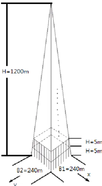
In order to study the behavior of pyramid-like tubular structure, the building structure shown in Fig. 4 is assumed. In the figure, the base of the structure is 240 m × 240 m and the height is 1200 m. This means the inclination of columns at pe-riphery of the structure is 1/10 in the horizontal x and y directions. The story height is 5 m. This leads to 240 stories for the structure. The building code of Taiwan (2006) is adopted to calculate the horizontal wind load. The wind pressure on the building is shown in Fig. 5. In the figure, the wind pressure is calculated by assuming 5% damping ratio for the structure.

Computer program SAP2000 is employed to model the pyramid-like structure. In the model, only beam element is used to model columns and spandrel beams, rigid diaphragms for all the floors are assumed, and the option of rigid zones at beam-column connections is selected. The members for the four corner columns are circular tubes with 200 cm in diameter and 6 cm, 8 cm or 10 cm in thickness. The members for the other periphery columns are 100cm × 50cm rectangular tube with 6 cm, 8 cm or 10 cm in thickness. In order to keep total area of corss sections of columns constant at periphery of the structure, the spacing of the columns is 3 m for the thickness 6 cm, the spacing of the columns is 4 m for the thickness 8 cm, and the spacing of the columns is 5 m for the thickness 10 cm. Three types of member are selected for the spandrel beams. The cross sections of the three types of beams are shown in Fig. 6. Therefore, one totally has 9 cases ( 3 different cross sections of spandrel beams times 3 different spacing of periphery columns ) to be studied. In the study, the vertical loading ( gravity loading ) is not taken into account. Therefore, only periphery columns and spandrel beams are modeled in Fig. 4 to resist the horizontal wind pressure shown in Fig. 5.

Fig. 4 Pyramid-like tubular building structure

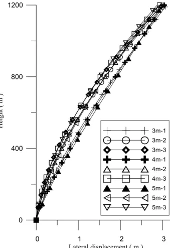
The lateral displacement due to the wind load of Fig. 5 is shown in Fig. 7. In the figure, the symbol 3m-1 represents the case with 3 m column spacing and spandrel beam type No. 1 of Fig. 6,

and the other similar symbols ( 3m-2 … etc. ) rep-resent the corresponding cases. From Fig. 7, one can observe the phenomenons as follow :

( 1 ) Stiffer spandrel beam will make the lateral displacement smaller. For examples, the sways for the cases 3m-3, 4m-3 and 5m-3 are smaller, while compared to the corresponding cases 3m-2, 4m-2 and 5m-2, and 3m-1, 4m-1 and 5m-1, respective-ly.

Fig.5 Design wind pressure by building code of Tai-wan(2006)

( 2 ) If the column area is more evenly distributed around the periphery, the sway is smaller. For ex-amples, results for the case 3m-1 is smaller than that for the cases 4m-1 and 5m-1.

( 3 ) However, the maximum lateral displacement at top of the building structure seems entangled for the 9 cases.

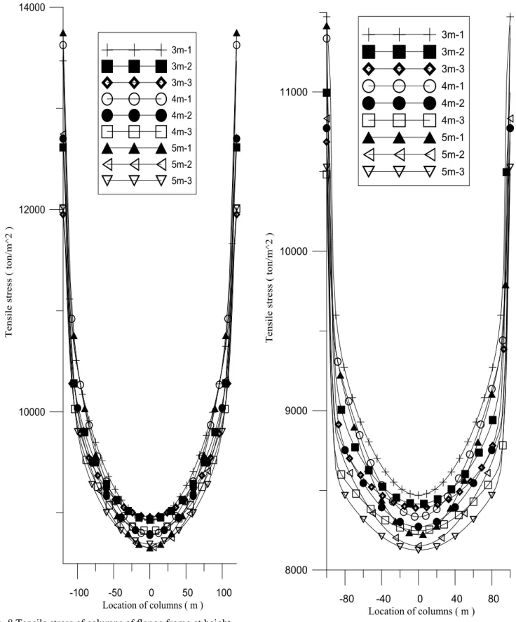
Fig. 8 shows the tensile stress of the columns of flange frame at height 0 m. In the figure, one can see that the curves for shear lag phenomenon can be divided into 3 groups for the 3 types of spandrel beams shown in Fig. 6 respectively. For stronger spandrel beam, the shear lag effect is lesser. For example, the shear lag phenomenon is lightest for the strongest spandrel beam ( Type No. 3 in Fig. 6 ). However, the effect of evenly distributed column area seems not so obvious to reduce shear lag phenomenon. This can be ob-served by comparing the results for cases of 3 m spacing to that for the corresponding cases of 4 m and 5 m spacings.

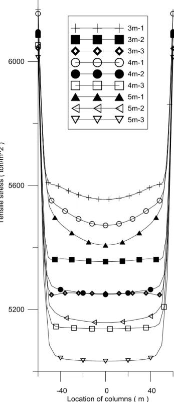
Figs. 9 and 10 show the tensile stress of col-umns at heights 200 m and 600 m respectively. From these two figures, one can observe that neg-ative shear lag phenomenon does not occurs for all 9 cases. As a matter of fact, there is no nega-tive shear lag observed along the height of the building, as one examines all the column stress. This could be the effect of inclination ofcolumns.

3 CONCLUDING REMARKS

The pyramid-like structural type is suitable for super tall building. It has the advantages to effec-tively reduce shear lag phenomenon along periph-ery columns and lateral displacement along the height of building. Also, this structural type can be easily combined with other structural forms, e.g. large scale bracing and outrigger structures, to re-sist horizontal wind load.

4 ACKNOWLEDGMENTS

The work is partly sponsored by National Science Council of Taiwan. The support is greatly appre-ciated.

5 REFERENCES

Ali, Mir M. & Kyoung, Sun Moon 2007. Structural Devel-opments in Tall Buildings : Current Trends and Future Prospects, Architectural Science Review Vol 50.3 : 205-223.

Building code of Taiwan. 2006.

Connor, J.J. & Pouangare, C.C. 1991. Simple Model for Design of Framed-Tube Structures, Journal of Struc-tural Engineering, ASCE, 117(12) : 3623-3644. Khan, F.R. & Amin, N.R. 1973. Analysis and design of

framed tube structures for tall concrete buildings, The Structural Engineer, Vol.51 : 85-92.

Singh, Y. & Nagpal, A.K. 1994. Negative Shear Lag in Framed-Tube buildings, Journal of structural Engi-neering, ASCE, 120(11) : 3105-3121.

User's manual of SAP 2000. 2000.

Wang, C.C. 2012. Parametric study of bundle tubular structures, Master Thesis ( In Chinese ).

Fig. 8 Tensile stress of columns of flange frame at height

0 m( 1st story) Fig. 9 Tensile stress of columns of flange frame at height 200 m

Fig. 10 Tensile stress of columns of flange frame at height 600 m

四、建議

參加國際會議不一定只參加大型會議，如小型且專門某一領域之會議，反而與國際知名的學者互動機 會較多。所以有些專門領域之會議亦應鼓勵參加。

五、攜回資料名稱及內容

(1)Conference Proceedings(此為每篇文章只有二頁之長摘要(long abstract)) (2)CD 之 Conference Proceedings(此為每篇完整之文章)

六、其他

無

國科會補助計畫衍生研發成果推廣資料表

日期:2013/12/29

國科會補助計畫

計畫名稱: 不均勻外力作用於層狀半空間內之解析解 計畫主持人: 劉俊秀 計畫編號: 101-2221-E-009-172- 學門領域: 結構應力

無研發成果推廣資料

101 年度專題研究計畫研究成果彙整表

計畫主持人：劉俊秀 計畫編號： 101-2221-E-009-172-計畫名稱：不均勻外力作用於層狀半空間內之解析解 量化 成果項目 實際已達成 數（被接受 或已發表） 預期總達成 數(含實際已 達成數) 本計畫實 際貢獻百 分比 單位 備 註 （ 質 化 說 明：如 數 個 計 畫 共 同 成 果、成 果 列 為 該 期 刊 之 封 面 故 事 ... 等） 期刊論文 0 0 100% 研究報告/技術報告 0 0 100% 研討會論文 0 0 100% 篇 論文著作 專書 0 0 100% 申請中件數 0 0 100% 專利 已獲得件數 0 0 100% 件 件數 0 0 100% 件 技術移轉 權利金 0 0 100% 千元 碩士生 0 0 100% 博士生 0 0 100% 博士後研究員 0 0 100% 國內 參與計畫人力 （本國籍） 專任助理 0 0 100% 人次 期刊論文 2 1 100% 研究報告/技術報告 0 0 100% 研討會論文 1 1 100% 篇 論文著作 專書 0 0 100% 章/本 申請中件數 0 0 100% 專利 已獲得件數 0 0 100% 件 件數 0 0 100% 件 技術移轉 權利金 0 0 100% 千元 碩士生 2 2 100% 博士生 1 1 100% 博士後研究員 0 0 100% 國外 參與計畫人力 （外國籍） 專任助理 0 0 100% 人次

其他成果

(

無法以量化表達之成 果如辦理學術活動、獲 得獎項、重要國際合 作、研究成果國際影響 力及其他協助產業技 術發展之具體效益事 項等，請以文字敘述填 列。) 無 成果項目 量化 名稱或內容性質簡述 測驗工具(含質性與量性) 0 課程/模組 0 電腦及網路系統或工具 0 教材 0 舉辦之活動/競賽 0 研討會/工作坊 0 電子報、網站 0 科 教 處 計 畫 加 填 項 目 計畫成果推廣之參與（閱聽）人數 0

國科會補助專題研究計畫成果報告自評表

請就研究內容與原計畫相符程度、達成預期目標情況、研究成果之學術或應用價

值（簡要敘述成果所代表之意義、價值、影響或進一步發展之可能性）

、是否適

合在學術期刊發表或申請專利、主要發現或其他有關價值等，作一綜合評估。

1. 請就研究內容與原計畫相符程度、達成預期目標情況作一綜合評估

■達成目標

□未達成目標（請說明，以 100 字為限）

□實驗失敗

□因故實驗中斷

□其他原因

說明：

2. 研究成果在學術期刊發表或申請專利等情形：

論文：□已發表 □未發表之文稿 ■撰寫中 □無

專利：□已獲得 □申請中 ■無

技轉：□已技轉 □洽談中 ■無

其他：（以 100 字為限）

投稿 Journal of Earthquake Engineering and Structure Dynamic

3. 請依學術成就、技術創新、社會影響等方面，評估研究成果之學術或應用價

值（簡要敘述成果所代表之意義、價值、影響或進一步發展之可能性）（以

500 字為限）

本研究主要突破為求得小面積內分佈載重之解析解,與 Green function 相較,本研究之解 沒有奇異(singularity)值問題。