總體經濟變數宣告日與非宣告日報酬差異之研究 - 政大學術集成

全文

(1)國立政治大學財務管理碩士班碩士論文. 治. 政總體經濟變數宣告日與非宣告日報酬差異之研究大. 立. ‧. ‧ 國. 學. A Tale of Two Days: Investor Sentiment or Risk ?. n. er. io. sit. y. Nat. al. Ch. engchi. i Un. v. 指導教授：湛可南教授研究生：連振廷撰. 中華民國 103 年 6 月.

(2) Abstract The returns of the days that macroeconomic news scheduled for release (announcement days) are extremely higher than those of other trading days. This paper reveals that investor sentiment is positively related to the excess returns difference and it predicts the difference of the returns. Also, investor sentiment is a significant factor to explain the excess returns difference during high sentiment period, whereas it is not significant during low sentiment period. Finally, we reconcile risk factor and sentiment. 政治大 important role in the excess returns difference between announcement days and other 立 factor toward the excess returns difference, suggesting that investor sentiment plays an. ‧. ‧ 國. 學. io. sit. y. Nat. n. al. er. days.. Ch. engchi. i Un. v.

(3) Content 1. INTRODUCTION....................................................................................................... 3 2. DATA AND METHODOLOGY .................................................................................. 7 2.1 ANNOUNCEMENT DAYS ..................................................................................................... 7 2.2 AGGREGATE MARKET RETURNS ........................................................................................ 7 2.3 INVESTOR SENTIMENT ....................................................................................................... 8 2.4 EXPECTED VARIANCE ........................................................................................................ 8 2.5 SUMMARY STATISTICS ........................................................................................................ 9 3 EMPIRICAL RESULTS .............................................................................................. 9 3.1 RETURN DIFFERENCE AND INVESTOR SENTIMENT .............................................................. 9 3.2 RETURN DIFFERENCE DURING HIGH SENTIMENT AND LOW SENTIMENT PERIOD ............... 12. 政治大 I S ? ........................................... 14. 3.3 THE PREDICTABILITY OF INVESTOR SENTIMENT ............................................................... 13. 立. 3.4 WHICH FACTORS MATTERS: RISK OR NVESTOR ENTIMENT. 4 ROBUSTNESS CHECKS .......................................................................................... 15. ‧ 國. 學. 4.1 USING VIX AND CLOSED-END FUND DISCOUNT FACTORS AS THE PROXY OF INVESTOR SENTIMENT ........................................................................................................................... 15. ‧. 4.2 TESTING VARIOUS PORTFOLIOS ....................................................................................... 17 4.3 CONTROLLING THE POTENTIAL EFFECT FROM FUNDAMENTAL INFORMATION .................. 18. y. Nat. sit. 5. CONCLUSION ......................................................................................................... 20. n. al. er. io. REFERENCE ............................................................................................................... 21. Ch. engchi. i Un. v. 1.

(4) LIST OF FIGURES: FIGURE 1. INVESTOR SENTIMENT INDEX FROM 1966 TO 2010.............................................................. 23. LIST OF TABLES: TABLE 1 SUMMARY STATISTICS OF DAILY STOCK MARKET EXCESS RETURNS ..................................... 24 TABLE 2 MONTHLY EXCESS RETURNS DIFFERENCE AGAINST INVESTOR SENTIMENT: ........................ 28 TABLE 3 MONTHLY EXCESS RETURNS DIFFERENCE AGAINST THE SIGN OF INVESTOR SENTIMENT .... 30 TABLE 4 MONTHLY EXCESS RETURNS DIFFERENCE AGAINST INVESTOR SENTIMENT DURING PERIODS OF HIGH AND LOW INVESTOR SENTIMENT.................................................................................... 32. TABLE 5 INVESTOR SENTIMENT AND MONTHLY EXCESS RETURNS DIFFERENCE: PREDICTIVE. 政治大. REGRESSIONS FOR INVESTOR SENTIMENT ON LONG-SHORT STRATEGY RETURNS. .................... 33. 立. TABLE 6 MONTHLY EXCESS RETURNS AGAINST CONDITIONAL VARIANCE AND INVESTOR SENTIMENT DURING EACH HIGH- AND LOW- SENTIMENT PERIODS ................................................................. 35. ‧ 國. 學. TABLE 7 MONTHLY EXCESS RETURNS DIFFERENCE AGAINST INVESTOR SENTIMENT: USING VIX AS PROXY OF INVESTOR SENTIMENT ................................................................................................. 36. ‧. TABLE 8 MONTHLY EXCESS RETURNS DIFFERENCE AGAINST INVESTOR SENTIMENT: USING THE CLOSED-END FUND DISCOUNT AS A PROXY OF INVESTOR SENTIMENT ........................................ 38. y. Nat. TABLE 9 MONTHLY EXCESS RETURNS DIFFERENCE AGAINST INVESTOR SENTIMENT DURING PERIODS. sit. OF HIGH INVESTOR SENTIMENT ................................................................................................... 40. al. er. io. TABLE 10A MONTHLY EXCESS RETURNS DIFFERENCE AGAINST INVESTOR SENTIMENT. v. n. (ORTHOGONAL): ........................................................................................................................... 42. Ch. i Un. TABLE 10B MONTHLY EXCESS RETURNS DIFFERENCE AGAINST INVESTOR SENTIMENT DURING. engchi. PERIODS OF HIGH AND LOW INVESTOR SENTIMENT (ORTHOGONAL). ......................................... 44. TABLE 10C MONTHLY EXCESS RETURNS AGAINST CONDITIONAL VARIANCE AND INVESTOR SENTIMENT (ORTHOGONAL) DURING EACH HIGH- AND LOW- SENTIMENT PERIODS .................. 45. 2.

(5) 1. Introduction Savor and Wilson (2012) document that the returns are extremely different between the days macroeconomic news scheduled for release (the following we use term “announcement-day” or “announcement days” ) and other trading days (the following we use term “non-announcement-day” or “non-announcement days”). Their study reveals that during period from 1963 to 2011 announcement-day earns 11 bps average daily excess returns whereas non-announcement-day earns only 1.1bps average daily excess returns, and that the sharp ratio in announcement-day is ten times to the ratio in non-announcement-day.. 政治大. Stocks returns should perform poorly when the news suggest that the market will. 立. turn to be bear, making the announcement days is risky than other days. For example,. ‧ 國. 學. recent studies document that interest rate, unemployment rate, and inflation rate strongly predict stock returns (Bernanke & Kuttner 2005; Ioannidis & Kontonikas. ‧. 2008; Bjørnland & Leitemo 2009; Birz & Lott 2011). When those indicators show. y. Nat. io. sit. good (bad) news, the market turns to be bull (bear). Also, when the indicators shows. n. al. er. weak (strong) signal about fundamental economics, investors tend to require higher. Ch. i Un. v. (lower) compensation of systematic risk. While economic announcements presumably. engchi. release important information about economy, the risk of such announcement days should be higher than that of other days so that higher returns on announcement days should be compensation for investors who bear macroeconomic risks. While several studies (Black 1972; Fama & French 1992; Black 1995; Polk et al. 2006) suggest no direct relation between the beta and the excess returns in most stocks, Savor and Wilson (2013), following intuition of macroeconomic risk on announcement days, explore the risk-returns trade off relation on such days. That is, they employ conditional variance to forecast the next period returns, showing that in announcement days beta successfully predicts the excess returns and that excess 3.

(6) returns holds traditional asset pricing theories. But as SW(2013) present, risk factor is possibly not the only factor to explain the difference excess returns between announcement-day and non-announcement-day because there exist much difference between these two types of days. For example, both individual investors and institutional investors extremely focus on the announcement of macroeconomics news, and the composition of those investors will be different between announcement days and other days (Pastor & Veronesi 2012). Once macroeconomic news announced monthly, analysts will write the analysis, comments, and expectation about the future, and then these contexts distribute by TV, magazine and several social media to lots of. 治政 investors, including professional investor and noise traders 大 (Kumar & Lee 2006). That 立 is, unlike in other days, in announcement days not only informative investor but also ‧ 國. 學. noise traders buy and sell in the market to hold their own portfolio (Black 1986).. ‧. Tetlock (2007) finds that the future market is less informative when Wall Street. sit. y. Nat. Journal releases news, this fact account for an increase in noise traders in that time.. io. al. er. Podolski–Boczar et al. (2009) reveal that noise traders will affect not the returns but the volatility. Those evidences suggest that the composition of investors is different. n. iv n C between announcement days and non-announcement U The different level of noise h e n g c h i days. trader, who affected by investor sentiment, should account for excess returns difference between two days. Follow this intuition, we propose two hypotheses. First, in the announcement days both sentiment driven noise traders and rational investors participate in the stock market, whereas less noise traders participate in non-announcement days. The different level of sentiment driven noise traders leads to different influence on excess returns (De Long et al. 1990; Shleifer & Summers 1990). We anticipate that investor sentiment will predict difference excess returns between two days because these noise traders are strongly affected by investor sentiment. Also, Brown and Cliff (2004) 4.

(7) reveal that changes in investor sentiment predicts future returns. Shleifer (2012) and Figlewski (1981) documents that investors usually follow “System 1” thinking, which means they decide to buy or to sell simply depends on first expression, to decide their strategy. This action links to the nearest feeling, changes in sentiment (Lee et al. 2002). That is, returns of announcement days will positively relate to changes in sentiment. On the other hand, the noise traders were also affected by status, weak or strong, of the market (Stambaugh et al. 2012). We define high and sentiment periods that depend on using sentiment index. During high sentiment period, noise traders will much strongly mispricing than in low sentiment. We expect that in high sentiment. 治政 investor sentiment positively related to returns of announcement 大 days whereas it does 立 not exist in low sentiment. ‧ 國. 學. In our research, we first present summary statistics of each announcement days. ‧. and non-announcement days. We use both equal-weighted portfolio and value-. sit. y. Nat. weighted portfolios. During 1966 to 2010 period, the monthly average excess daily. io. al. er. returns of value-weighted portfolio is 1.46% in announcement days versus only 0.28% in non-announcement days. The difference excess returns is significant with t-. n. iv n C statistics 2.10 of value-weighted portfolio. Then we regress the different excess heng chi U. returns on the changes in investor sentiment index, reporting that investor sentiment is a significant factor both in controlling and non-controlling equations with at least tstatistics 2.19. Also, we test different proxies of investor sentiment, such as VIX and closed-end fund (Lee et al. 1991) discount, revealing strong significance as well as above. Besides, we use time series regression to test predictability of investor sentiment on long-short strategy, a strategy that long announcement day and short non-announcement day, and we show that investor sentiment successfully predicts the returns of strategy in time t+1. These results suggest investor sentiment is positively correlated to difference excess returns between announcement days and non5.

(8) announcement days, and it also predict future returns. We then examine the second hypothesis: investor sentiment works during high sentiment period rather than does during low sentiment. We classified high- and lowinvestor sentiment periods based on the median level of the index of Baker and Wurgler (2006), and we regress equations during each high- and lowsentiment periods. Our reports show that each of t-statistics of sentiment estimate is significant during high investor sentiment, and that none of t-statistics of estimate of sentiment is significant during low investor sentiment. To show that our result is strongly robust, we use various portfolios, which include portfolios formed by industry, size, book-to-. 治政 market(Fama & French 1992), momentum, to test, suggesting 大 the results still hold on 立 most of such different portfolio in high sentiment, especially in small firms (Lemmon ‧ 國. 學. & Portniaguina 2006). These results suggest investor sentiment is positively. ‧. correlated to difference excess returns between announcement days and non-. sit. y. Nat. announcement days during high sentiment period rather than in low sentiment period.. io. al. er. “A tale of two days” leads different patterns, the patterns account not only for the risk story that SW proposed but, significantly, for the sentiment driven factors such as. n. iv n C noise trader and investor sentiment.hAs Lakonishok etU e n g c h i al. (1994) suggests, we. consider the factors other than risk as explanation when we find that risk-returns trade off relation does not always hold. We adapt the methodology that proposed in Savor and Wilson (2012). In our methodology, we regress –by each high- and lowsentiment – announcement-day aggregate excess returns in quarter t+1 on expected variance, which is in quarter t, and on investor sentiment, which is also in quarter t. Our report suggests that the expected variance predicts the returns only during low sentiment period, and instead investor sentiment predicts the returns during high sentiment. This fact implies investor sentiment plays an important role in the difference excess returns between announcement days and non-announcement days. 6.

(9) In this papers, we provide investor sentiment explanation toward a tale of two days puzzle. We show that investor sentiment empirically accounts for difference excess returns between announcement days and predicts returns on long-short strategy portfolio, and that different excess returns interact with investor sentiment index during high sentiment period. Finally, we reconcile the relation between risk factors and sentiment factors. The rest of the paper is organized as follows. Section 2 describes data and introduces methodology. Section 3 reports the main empirical results and Section 4 gives the result robust test. Section 5 concludes.. 立. 政治大. 2. Data and Methodology. ‧ 國. 學. 2.1 Announcement Days. ‧. We define, following definition of Savor and Wilson (2012), macroeconomic. y. Nat. sit. news announcement day, including scheduled announcement days of Consumer Price. n. al. er. io. Index(CPI), unemployment rate, and FOMC meeting that releases interest rate. i Un. v. decision. We obtain Consumer Price Index and Producer Price Index (PPI) data from. Ch. engchi. the Bureau of Labor Statistics’ website as the inflation rate announcement. Consumer Price Index start from 1958 to 1972 and Producer Price Index (PPI) start from 1972. FOMC scheduled meeting of the interest rate started from 1978. Unemployment rate started from 1958. 2.2 Aggregate Market Returns We obtain stock returns data from CRSP. Our main stock market proxy is the CRSP NYSE/AMEX/NASDAQ value-weighted index and equal-weighted index of all listed shares. We also obtain 5 industry portfolio, 18 size-sorted portfolios, 18 7.

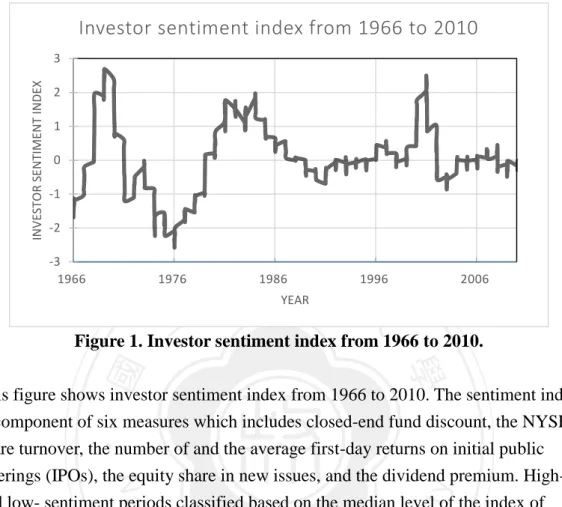
(10) book-to-market-sorted portfolio, 2*3 size/book-to-market portfolios, 2*3 size/momentum portfolio from Kenneth French website. All proxies start from 1966 to 2010. 2.3 Investor Sentiment We use the changes in investor sentiment index that Baker and Wurgler (2007) formed. The sentiment index composite of six measures: closed-end fund discount, the NYSE share turnover, the number of IPOs, the average first-day returns of IPOs, the equity share in new issues, and the dividend premium. The sentiment index is. 政治大. from 1966 to 2010.. 立[Figure 1 INSERT HERE]. ‧ 國. 學. Using the index, we identify the late 1960s, mid-1980s, and late 1990s, and early. sit. y. Nat. & Wurgler 2006), and identify others as low sentiment period.. ‧. 2000s as high sentiment period in which investor sentiment more than median(Baker. io. al. er. Besides, we consider closed-end fund discount(Chopra et al. 1993), VIX(Simon & Wiggins 2001) as another measures of investor sentiment to do robust tests. Closed-. n. iv n C end fund discount start from 1966 to start from 1990 to 2010. h2010, e n gandcVIX hi U 2.4 Expected variance. We use expected variance that follows rolling window model (French et al. 1987)to exam risk-returns trade off. The conditional variance use realized variance of the current month for next month’s returns.. 8.

(11) 2.5 Summary Statistics Using the time series data, we first identify announcement days and other days. We set dummy as 1 if there is either inflation rate, unemployment rate, or interest rate announcement scheduled, and other sent dummy as zero. Then we set time series tag monthly: calculate average daily returns of each type of days monthly and times 22, the approximate number of trading days in one month. The descriptive statistics of each day and pair T test shows below: [Table 1 INSERT HERE]. 治政 We document 539 samples from 1966 to 2010 monthly, 大 exclude July in 1968 in 立 which no announcement occurs. This result shows that value-weighted market returns ‧ 國. 學. average earn 1.45% in announcement days versus 0.27% that earned in other days,. ‧. suggesting a significant difference within two type of days. Like value-weighted. sit. y. Nat. market returns, equal-weighted market returns similarly average earn 2.65% in. io. al. er. announcement days versus 1.05% in other days, suggesting difference with t statistics. n. equal 3.66. Either value-weighted or equal-weighted stock returns imply the. i n C days difference between announcement and other days. U hengchi. v. 3 Empirical Results 3.1 Return difference and investor sentiment The investor sentiment has been intensively analyzed in the following two equations A𝑖,𝑡 − N𝑖,𝑡 = a𝑖 + bSENT𝑡 + cRMTRF𝑡 + ϵ𝑖,𝑡. (1). A𝑖,𝑡 − N𝑖,𝑡 = a𝑖 + bSENT𝑡 + cRMTRF𝑡 + dSMB𝑡 + + ϵ𝑖,𝑡. (2). A𝑖,𝑡 − N𝑖,𝑡 = a𝑖 + bSENT𝑡 + cRMTRF𝑡 + dSMB𝑡 + eHML𝑡 + ϵ𝑖,𝑡. (3) 9.

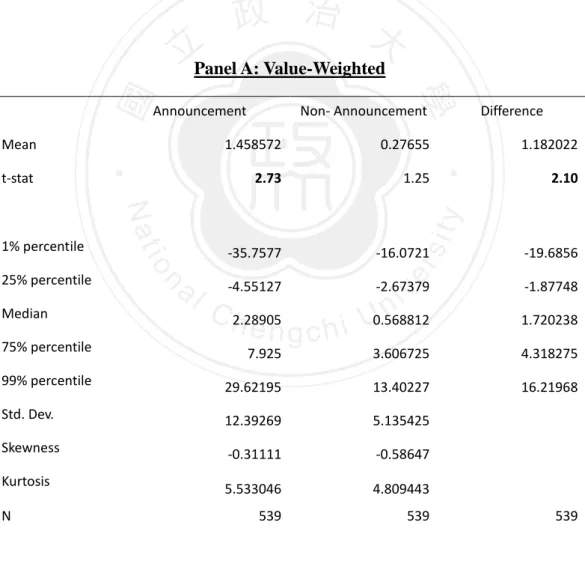
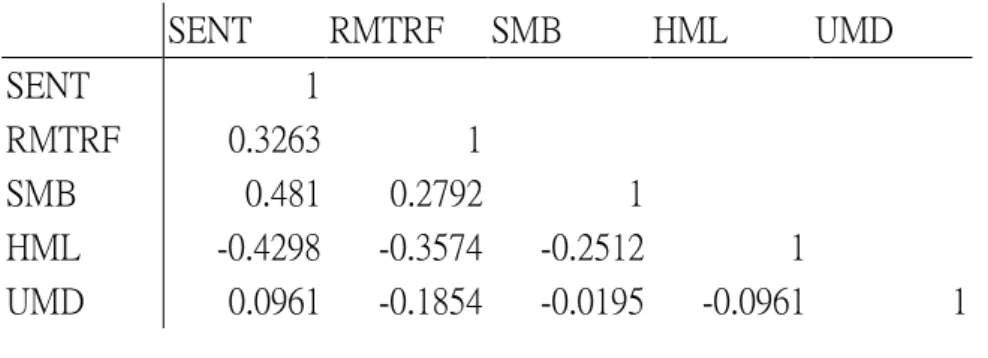
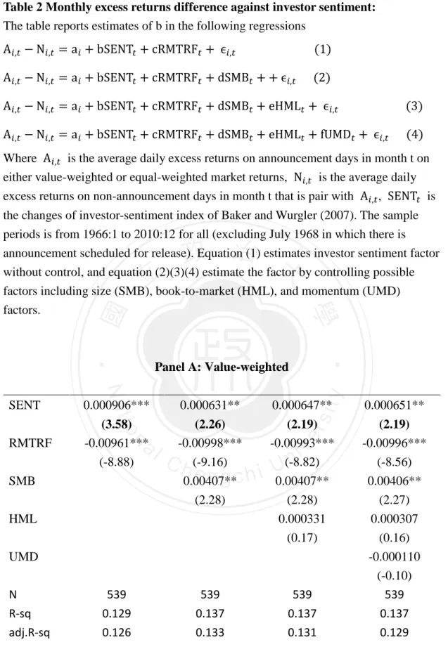
(12) A𝑖,𝑡 − N𝑖,𝑡 = a𝑖 + bSENT𝑡 + cRMTRF𝑡 + dSMB𝑡 + eHML𝑡 + fUMD𝑡 + ϵ𝑖,𝑡. (4). Where Ai,t is the monthly excess returns in announcement days and Ni,t is the monthly excess returns in non-announcement days. Where RMTRFt represents market risk premium. In the second equation, we use SMBt and HMLt to control the size effect and value effect(Fama & French 1996). Where SENTt represent changes in investor sentiment at time t. We examine the correlation and VIF between factors as below [Table1B&1C INSERT HERE] The empirical result shows below: [Table 2 INSERT HERE]. 治政 In the value-weighted panel, result reveal that sentiment 大 factor is significant with 立 coefficient 0.000906 and t-ratio 3.58, suggesting investor sentiment positive ‧ 國. 學. correlated spread between announcement days and other days. The R-square. ‧. represents 0.126. Next, we consider size effect and value effect so that we regress. sit. y. Nat. with control SMB and HML factor. We find that investor sentiment factor is still. io. al. er. significantly positively related spread with t-ratio 2.26 and 2.19 each model. The Rsquare about those equations is 0.137. Even, we consider possible factor momentum. n. iv n C (UMD), investor sentiment still plays role to explain spread with t-ratio h eannimportant gchi U 2.19 and R-square 0.137. We then use the same model to test in equal-weighted panel. The result reveal that investor sentiment factor significantly positively related to spread. In the full equation, investor sentiment factor is significant with coefficient 0.00062 and t-ratio 3.09. The R-square is 0.105. After control size effect and value effect, sentiment factor is still significant with coefficient 0.000637 and 0.000596, and with t-ratio 2.86 and 2.54. Even we control momentum factor, the investor sentiment factor is still significant with coefficient 0.00059 and t-ratio 2.50 Following our hypothesis, we then use dummy to represent changes in investor 10.

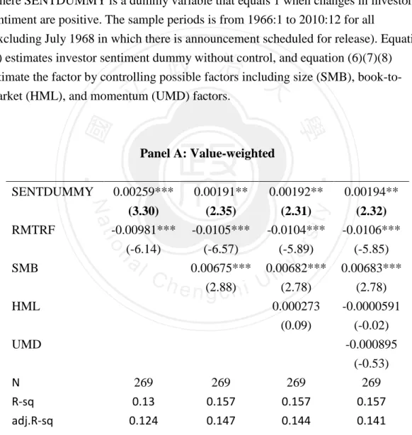
(13) sentiment. As we proposed in the Section 1, when investor feels better, they tend to buy in and overprice (Kaniel et al. 2008), leading to high spread between announcement days and other days, these days exist different level of noise trader. We use dummy variable. The variable equals 1 when changes in sentiment is positive, and variable equals zero when changes in sentiment is negative or zero. Run the regression A𝑖,𝑡 − N𝑖,𝑡 = a𝑖 + bSENTDUMMY𝑡 + cRMTRF𝑡 + ϵ𝑖,𝑡. (5). A𝑖,𝑡 − N𝑖,𝑡 = a𝑖 + bSENTDUMMY𝑡 + cRMTRF𝑡 + dSMB𝑡 + ϵ𝑖,𝑡. (6). A𝑖,𝑡 − N𝑖,𝑡 = a𝑖 + bSENTDUMMY𝑡 + cRMTRF𝑡 + dSMB𝑡 + eHML𝑡 + ϵ𝑖,𝑡 𝑖,𝑡. 𝑖. 𝑡. 𝑡. 𝑡. [Table 3 INSERT HERE]. 𝑡. 𝑡. 𝑖,𝑡. (7) (8). 學. ‧ 國. A𝑖,𝑡. 治政 − N = a + bSENTDUMMY + cRMTRF + dSMB + 大eHML + fUMD + ϵ 立 The empirical reports shows below: ‧. In the report, we find value weighted spread positively related to investor. sit. y. Nat. sentiment dummy variable with t-ratio 3.30. After controlling size effect, investor. io. al. er. sentiment dummy is positive and significant with t-vale 2.35. Controlling both size effect and value effect, investor sentiment dummy is still positive and significant with. n. iv n C t-vale 2.31. We obtain same result by all the possible factor. In the equalh econtrolling ngchi U weighted panel, the table shows similar result as those in value-weighted panel, a. result that investor sentiment positively related to spread between announcement days and other days. From the empirical result, it strongly indicate that investor sentiment strongly positively related to the spread, suggesting that investor influenced by sentiment so that mispricing stocks. When investors feel better in the period, they overpricing the stocks whereas investors feel worse, they underpricing the stock price.. 11.

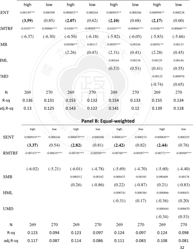
(14) 3.2 Return difference during high sentiment and low sentiment period We proposed that noise traders in the high sentiment period will perform much strongly than in the low sentiment period. We test the how sentiment affect spread during each period. [Table 4 INSERT HERE]. 治政 In table 4, in the high sentiment panel, as we proposed, 大 investor sentiment 立 influent spread significantly. Investor sentiment positively related to spread with ‧ 國. 學. coefficient 0.0013 and t-ratio 3.59 in the full equation of value-weighted market. ‧. returns. After controlling size effect, we find that the coefficient of investor sentiment. sit. y. Nat. factor is still significant with t-ratio 2.07. Even we control value factor, and. io. al. er. momentum factor from factor model, investor sentiment factor is still significant with t-ratio 2.10 and 2.17, suggesting that investor sentiment factor explains the spread of. n. iv n C two types of days. Like value-weighted returns, equal weighted returns h e market ngchi U. reported consistent result that investor sentiment positively related to market returns with coefficient 0.000919 and t-ratio 3.37 in the full equation, and that sentiment factor is still significant with t-ratio at least 2.42 in the controlling equation. Whereas investor sentiment impacts strongly on spread of two types of days during high sentiment period, there exist no relation, as we proposed in the Section1, in low sentiment period. In the table 4, we find in the value-weighted panel that investor sentiment has positive coefficient with spread but t-ratio is only around 0.6 in controlling equation. Even we use full equation to regress, the result still, consistently reveal insignificantly with t-ratio 0.85. On the other hand, our test on equal-weighted 12.

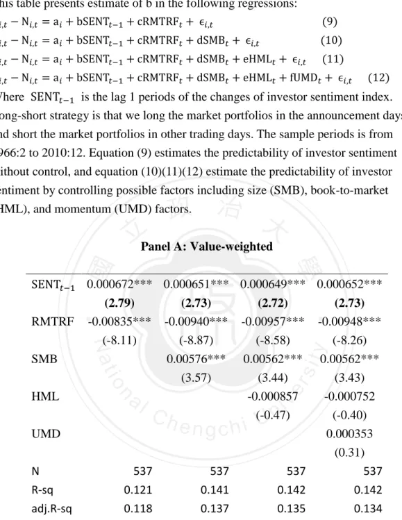
(15) reveal similar result that investor sentiment factor, no matter control or not, did not plays a role in the spread between each types of days. These results are strongly consistent with our expectation: sentiment driven noise traders act strongly during high sentiment period rather than during low sentiment period. In the above empirical test, value-weighted market returns and equal-weighted returns show similar result. Moreover, both controlling equations and full equation show same result. 3.3 The predictability of investor sentiment. 治政 Whereas the sentiment factor explains the spread 大 between each types of days, we 立 proposed, basing on autocorrelation of investor sentiment, exam the predictability ‧ 國. 學. toward spread of market returns. Intuitively, it is unusual that investor sentiment. ‧. changes frequently between continued months, and instead the investor sentiment. y. Nat. exists a high autocorrelation with itself between months. Test the follow regresses. n. al. Ch. er. io. A𝑖,𝑡 − N𝑖,𝑡 = a𝑖 + bSENT𝑡−1 + cRMTRF𝑡 + dSMB𝑡 + ϵ𝑖,𝑡. (9). sit. A𝑖,𝑡 − N𝑖,𝑡 = a𝑖 + bSENT𝑡−1 + cRMTRF𝑡 + ϵ𝑖,𝑡. n engchi U. iv. (10). A𝑖,𝑡 − N𝑖,𝑡 = a𝑖 + bSENT𝑡−1 + cRMTRF𝑡 + dSMB𝑡 + eHML𝑡 + ϵ𝑖,𝑡. (11). A𝑖,𝑡 − N𝑖,𝑡 = a𝑖 + bSENT𝑡−1 + cRMTRF𝑡 + dSMB𝑡 + eHML𝑡 + fUMD𝑡 + ϵ𝑖,𝑡. (12). We use the lead 1 month investor sentiment to predict the spread between each types of days. [Table 5 INSERT HERE] In the report, using 537 samples, we find that investor sentiment strongly predict the next period returns with t-ratio 2.79 in full equation. Then, we test model that control size effect, investor sentiment factor still reports good predictability with tratio 2.73 and coefficient 0.000651. Controlling the value effect and momentum factor, we find that investor sentiment successfully predict spread of market returns. 13.

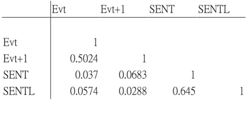
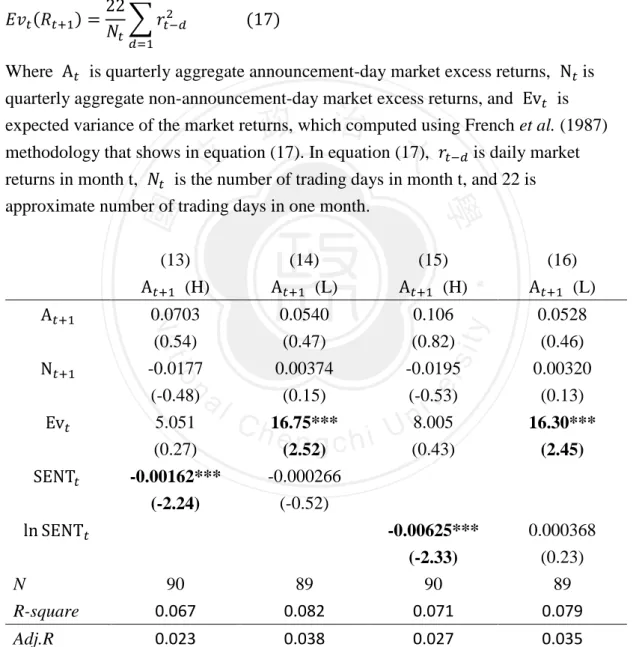
(16) Like value-weighted market returns, equal-weighted returns shows the similar result. In the full equation, investor sentiment predict significantly spread of each types of days with t-ratio 0.217 and coefficient 0.000414. After controlling each possible factors, we find that investor sentiment still significantly predict spread of returns with t-vale at least 2.12 and coefficient around 0.0004. These result strongly indicated that investor sentiment has significant predictability to spread of each types of days. 3.4 Which factors matters: Risk or Investor Sentiment? While Savor and Wilson (2012) suggest risk and returns trade off in the. 治政 announcement days, our result strongly indicate that investor 大 sentiment plays an 立 important role in the abnormal returns between announcement days and other days. ‧ 國. 學. Follow our result, because of existence of noise trader, unlike other days,. ‧. announcement days affected by investor sentiment, especially in high sentiment. That. sit. y. Nat. is, we here test the risk and sentiment factor in each period to exam the property of sentiment-driven noise trader.. n. al. (13)(ℎ𝑖𝑔ℎ 𝑠𝑒𝑛𝑡𝑖𝑚𝑒𝑛𝑡). er. io. A𝑡+1 = A𝑡 + N𝑡 + Ev𝑡 + SENT𝑡 A𝑡+1 = A𝑡 + N𝑡 + Ev𝑡 + SENT𝑡 A𝑡+1 = A𝑡 + N𝑡 + Ev𝑡 + ln SENT𝑡 A𝑡+1 = A𝑡 + N𝑡 + Ev𝑡 + ln SENT𝑡. (14)(𝑙𝑜𝑤 𝑠𝑒𝑛𝑡𝑖𝑚𝑒𝑛𝑡) iv n C h (15)(ℎ𝑖𝑔ℎ i U e n g c h𝑠𝑒𝑛𝑡𝑖𝑚𝑒𝑛𝑡) (16)(𝑙𝑜𝑤 𝑠𝑒𝑛𝑡𝑖𝑚𝑒𝑛𝑡). Here we use aggregate quarterly log excess returns to test. Where At+1 means returns of announcement days at time t+1. At means quarterly aggregate log excess returns in announcement days, and Nt means quarterly aggregate log excess returns in non-announcement days. The correlation and VIF showed below: [Table 1D&1E INSERT HERE]. The result shows below [Table 6 INSERT HERE] 14.

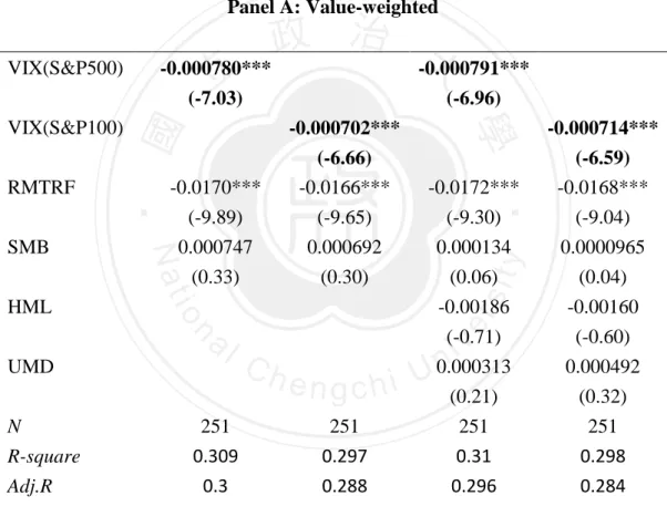
(17) We find from equation (13) that during high sentiment period, expected variance will not predict returns, and instead investor sentiment do so , and from equation (14) that during low sentiment period, the returns and expected variance exist risk returns trade off with insignificant investor sentiment factor. To precisely check the result, we use log sentiment index to test again, suggesting that during high sentiment period, investor sentiment successfully predicts the future returns, although there is risk returns trade off during low sentiment period. These results suggest that, besides risk factor, investor sentiment factor plays an important role to explain abnormal returns spread between each type of days. It was. 治政 true that it exist risk returns trade off relation between 大 expected variance and future 立 returns. However, our empirical indicate that it only exist in low sentiment period, ‧ 國. 學. when there is less noise trader, and that investor sentiment significantly explain the. ‧. excess returns difference between announcement days and non-announcement days.. y. Nat. sit. 4 Robustness checks. n. al. er. io. In this chapter, we present the results of robustness checks. In section 4.1, we. i Un. v. investigate how different investor sentiment proxy affect result. In section 4.2, we. Ch. engchi. break down our sample, testing with as much as 55 portfolio formed by size, value, and other factors. 4.1 Using VIX and closed-end fund discount factors as the proxy of investor sentiment In section 3 we show analyze and show that investor sentiment explain and predict spread of each types of days by using the index provided by Baker and Wurgler (2006). Does other investor sentiment indicator show similar ability? First, we examine with VIX index, an index also known as fear indicators. Here we regress the return difference on the change of VIX index. 15.

(18) A𝑖,𝑡 − N𝑖,𝑡 = a𝑖 + bVIX 𝑡 + cRMTRF𝑡 + ϵ𝑖,𝑡. (18). A𝑖,𝑡 − N𝑖,𝑡 = a𝑖 + bVIX 𝑡 + cRMTRF𝑡 + dSMB𝑡 + eHML𝑡 + fUMD𝑡 + ϵ𝑖,𝑡. (19). [Table 7 INSERT HERE] In the value-weighted full equation, both VIX index significantly explained the spread between each types of days with -0.00079 coefficient and t-ratio at least -6.59. We then use the highest adjust R-squared controlling equation, which was the equation controlling size effect, to examine, suggesting consistently that VIX negatively related to spread of each types of days with at least t-ratio -5.56. Besides, in the value-weighted market returns, the report reveal the similar. 治政 result: both VIX shows significantly relation with spread 大of two types of days. In full 立 equation, VIXS&P100 negatively related to equal-weighted market returns, with ‧ 國. 學. coefficient -0.0007 and t-ratio -6.59. In equation that controls size effect, VIXS&P100. ‧. still negatively related to equal-weighted market returns, with coefficient -0.0007 and. sit. y. Nat. t-ratio -6.66. We find similar result by replacing with VIX of S&P500. That is, VIX of. io. controlling.. al. er. S&P500 is significantly to explained market returns both in the full equation and. n. iv n C The negative sign of coefficient the definition. The higher the VIX h result e n gfrom chi U. index is, the lower sentiment belongs investor. Closed-end fund discount is also a popular proxy as investor sentiment. That is, when investor sentiment of individual investor is high, the discount of close-end fund will increase because individual investor buy the stocks directly from market(Fisher & Statman 2000). We examine by these equations A𝑖,𝑡 − N𝑖,𝑡 = a𝑖 + b𝑐𝑒𝑓𝑑𝑡 + cRMTRF𝑡 + ϵ𝑖,𝑡. (20). A𝑖,𝑡 − N𝑖,𝑡 = a𝑖 + b𝑐𝑒𝑓𝑑𝑡 + cRMTRF𝑡 + dSMB𝑡 + ϵ𝑖,𝑡. (21). A𝑖,𝑡 − N𝑖,𝑡 = a𝑖 + b𝑐𝑒𝑓𝑑𝑡 + cRMTRF𝑡 + dSMB𝑡 + eHML𝑡 + ϵ𝑖,𝑡. (22) 16.

(19) A𝑖,𝑡 − N𝑖,𝑡 = a𝑖 + b𝑐𝑒𝑓𝑑𝑡 + cRMTRF𝑡 + dSMB𝑡 + eHML𝑡 + fUMD𝑡 + ϵ𝑖,𝑡. (23). Where cefd is the closed-end fund discount. Table 8 is the empirical results: [Table 8 INSERT HERE] In the value-weighted market returns, the results suggest that the closed-end fund discount positively related spread of each types of days with t-ratio 2.19 in full equation, and that closed-end fund discount is also significant to explain spread with t-ratio at least 2.15 in the controlling equations that control size effect, value effect and momentum effect. Use equal-weighted market returns, we find similar result that closed-end fund discount strongly related to spread of each types of days with positive sign.. 立. 政治大. robustly consistent with our main result.. 學. ‧ 國. We test three index as investor sentiment proxy, suggesting that those results are. ‧. 4.2 Testing Various portfolios. sit. y. Nat. io. al. er. In this chapter, we test the power of each type of portfolio. During all portfolio test, we find 37 out of 55 portfolio shows that investor sentiment positively related to. n. iv n C spread of two types of days. Precisely, about investor sentiment that work h ewenconsider gchi U extremely on small size firm and low book-to-market ratio firm (Value stock), and then we find result that suggest 22 out of 23 portfolio with those feature are strongly significant. That is, investor sentiment holds on market, especially in small firm and growth firm, those firm that were difficult to value. Table 9 is the empirical results. [Table 9 INSERT HERE] Panel A shows the result of size-formed portfolio. We use three subgroup including trisections, quintile, and 10 equal size-form portfolio. In the first row, it shows that small firms is significant with t-ratio equals 2.8 versus 1.97 in big firm portfolio. In the second role, it reports that small firms is significant with t-ratio 17.

(20) equals 2.84 versus 1.90 in big firm portfolio. In the third row, it indicates that small firms is significant with t-ratio equals 2.69 versus 1.80 in big firm portfolio. Generally, in small firms investor sentiment much significantly explain the spread of each type of days. Panel B shows the result of value-formed portfolio. We use three subgroup that is similar with size-formed portfolio. In the first row, it shows that negative book-tomarket ratio and low boot-to-market ratio firms, also named growth firms, are significant with t-ratio equals 2.68 versus 0.98 in value firms portfolio. In the second role, it reports that growth firms is significant with t-ratio equals 2.35 versus 0.95 in. 治政 value firm portfolio. In the third row, it indicates that growth 大 firms portfolio is 立 significant with t-ratio equals 2.23 versus 1.07 in big firm portfolio. ‧ 國. 學. Panel C we use 2*3 size and value formed, and 2*3 size and momentum formed. ‧. portfolio examine. Clearly, in the small size and growth stock portfolios, they. sit. y. Nat. represent investor sentiment positively related to portfolio returns spread between. io. al. market ratio, represents highest t-ratio that equals 3.32.. er. each types of days. Portfolio that is with both two feature, small size and low book-to-. n. iv n C In these 55 portfolio test, we find investor sentiment holds on various type of h ethat ngchi U. portfolio, especially, as scholar document, on such firms that were difficulty to value(Baker & Wurgler 2006). The results are extremely consistent with our main idea: sentiment driven spread of two type of days because of sentiment driver noise trader.. 4.3 Controlling the potential effect from fundamental information To reduce the possibility that the investor sentiment index we used above correlated to fundamental effect, we test the result by using an orthogonal investor 18.

(21) sentiment index to do robustness checks in this chapter. The orthogonal investor sentiment index not only consists of the same six components of the former sentiment index we used, but also regress on growth in industrial production index, consumer durables, nondurables, and services, and a dummy variable for NBER recessions to remove potential fundamental information. [Table 10A INSERT HERE] We use this orthogonal investor sentiment index to regress on return difference. Table 10A shows that the index is positively correlated to the return difference, with coefficient (positive sign) 0.0004 and t-value 1.79.. 治政大 [Table 10B INSERT HERE] 立 Follow our hypothesis, we then test the relation between investor sentiment ‧ 國. 學. index (orthogonal) and return difference during each high- or lowsentiment period.. ‧. Table 10B shows that both in the value-weighted and in the equal-weighted panel,. io. y. sit. sentiment period than low sentiment period.. er. Nat. investor sentiment are much significantly related to return difference during high. n. 10C INSERT HERE] a[Table iv l C n Using the orthogonal investor h sentiment index, we e n g c h i Uexam how investor sentiment and risk influence the return difference. Table 10C suggests that during high sentiment period, investor sentiment index is significantly predicted to next period returns of announcement days with t-value -2.21 whereas during low sentiment period, expected variance successfully predicts the returns. These results imply that a risk-return tradeoff relation during low sentiment period, and that investor sentiment is a potential explanation during high sentiment period. Above checks indicate our hypothesis and examination are strongly robust. The robust test results are consistent with our test in Section 3, suggesting our finding is convincing. 19.

(22) 5. Conclusion In our paper we suggest that investor sentiment positively predicts, because of different level of noise trader, excess returns between announcement days and nonannouncement days. In the high sentiment period, investor sentiment plays an extremely important roles in the excess returns difference between days. We use forty eight portfolios to provide robust check with these results. Moreover, we provide evidence that investor sentiment factors holds during high sentiment period, reconciling traditional risk factors with behavioral factors.. 立. 政治大. ‧. ‧ 國. 學. n. er. io. sit. y. Nat. al. Ch. engchi. i Un. v. 20.

(23) Reference Baker, M., Wurgler, J., 2006. Investor Sentiment and the Cross-Section of Stock Returns. The Journal of Finance 61, 1645-1680. Baker, M., Wurgler, J., 2007. Investor sentiment in the stock market. Journal of Economic Perspectives 21, 129-151. Bernanke, B.S., Kuttner, K.N., 2005. What explains the stock market's reaction to Federal Reserve policy? The Journal of Finance 60, 1221-1257. Birz, G., Lott, J.R., 2011. The effect of macroeconomic news on stock returns: New evidence from newspaper coverage. Journal of Banking & Finance 35, 27912800. Bjørnland, H.C., Leitemo, K., 2009. Identifying the interdependence between US monetary policy and the stock market. Journal of Monetary Economics 56, 275-282. Black, F., 1972. Capital market equilibrium with restricted borrowing. Journal of. 政治大. business, 444-455. Black, F., 1986. Noise. The Journal of Finance 41, 529-543. Black, F., 1995. Estimating expected return. Journal of Financial Education, 1-4. Brown, G.W., Cliff, M.T., 2004. Investor sentiment and the near-term stock market. Journal of Empirical Finance 11, 1-27. Chopra, N., Lee, C.M.C., Shleifer, A., Thaler, R.H., 1993. Yes, Discounts on Closed-End Funds Are a Sentiment Index. The Journal of Finance 48, 801-808. De Long, J.B., Andrei, S., Lawrence, H.S., Robert, J.W., 1990. Noise Trader Risk in. 立. ‧. ‧ 國. 學. sit. y. Nat. n. al. er. io. Financial Markets. Journal of Political Economy 98, 703-38. Fama, E.F., French, K.R., 1992. The Cross-Section of Expected Stock Returns. The Journal of Finance 47, 427-465. Fama, E.F., French, K.R., 1996. Multifactor Explanations of Asset Pricing Anomalies. The Journal of Finance 51, 55-84. Figlewski, S., 1981. The Informational Effects of Restrictions on Short Sales: Some Empirical Evidence. Journal of Financial and Quantitative Analysis 16, 463-476 Fisher, K.L., Statman, M., 2000. Investor sentiment and stock returns. Financial Analysts Journal, 16-23. French, K.R., Schwert, G.W., Stambaugh, R.F., 1987. Expected stock returns and. Ch. engchi. i Un. v. volatility. Journal of Financial Economics 19, 3-29. Ioannidis, C., Kontonikas, A., 2008. The impact of monetary policy on stock prices. Journal of Policy Modeling 30, 33-53. Kaniel, R.O.N., Saar, G., Titman, S., 2008. Individual Investor Trading and Stock Returns. The Journal of Finance 63, 273-310. Kumar, A., Lee, C.M.C., 2006. Retail Investor Sentiment and Return Comovements. 21.

(24) The Journal of Finance 61, 2451-2486. Lakonishok, J., Shleifer, A., Vishny, R.W., 1994. Contrarian Investment, Extrapolation, and Risk. The Journal of Finance 49, 1541-1578. Lee, C.M.C., Shleifer, A., Thaler, R.H., 1991. Investor Sentiment and the Closed-End Fund Puzzle. The Journal of Finance 46, 75-109. Lee, W.Y., Jiang, C.X., Indro, D.C., 2002. Stock market volatility, excess returns, and the role of investor sentiment. Journal of Banking & Finance 26, 2277-2299. Lemmon, M., Portniaguina, E., 2006. Consumer Confidence and Asset Prices: Some Empirical Evidence. Review of Financial Studies 19, 1499-1529. Pastor, L.U., Veronesi, P., 2012. Uncertainty about Government Policy and Stock Prices. The Journal of Finance 67, 1219-1264. Podolski–Boczar, E., Kalev, P.S., Duong, H.N., 2009. Deafened by Noise: Do Noise Traders Affect Volatility and Returns? Working paper, Monash University. Polk, C., Thompson, S., Vuolteenaho, T., 2006. Cross-sectional forecasts of the equity. 政治大 premium. Journal of Financial Economics 81, 101-141. 立 Savor, P., Wilson, M., 2013. How Much Do Investors Care About Macroeconomic ‧. ‧ 國. 學. Risk? Evidence from Scheduled Economic Announcements. Journal of Financial and Quantitative Analysis 48, 343-375. Savor, P., Wilson, M.I., 2012. Asset pricing: A tale of two days. Journal of Financial Economics, forthcoming. Shleifer, A., 2012. Psychologists at the Gate: Review of Daniel Kahneman’s Thinking, Fast and Slow. Journal of Economic Literature 50, 1080-1091.. sit. y. Nat. n. al. er. io. Shleifer, A., Summers, L.H., 1990. The Noise Trader Approach to Finance. Journal of Economic Perspectives 4, 19-33. Simon, D.P., Wiggins, R.A., 2001. S&P futures returns and contrary sentiment indicators. Journal of Futures Markets 21, 447-462. Stambaugh, R.F., Yu, J., Yuan, Y., 2012. The short of it: Investor sentiment and anomalies. Journal of Financial Economics 104, 288-302. Tetlock, P.C., 2007. Giving Content to Investor Sentiment: The Role of Media in the Stock Market. The Journal of Finance 62, 1139-1168.. Ch. engchi. i Un. v. 22.

(25) Investor sentiment index from 1966 to 2010 INVESTOR SENTIMENT INDEX. 3 2 1 0 -1 -2 -3 1966. 1976. 立. 政治大 1986. 1996. 2006. YEAR. Figure 1. Investor sentiment index from 1966 to 2010.. ‧ 國. 學. ‧. This figure shows investor sentiment index from 1966 to 2010. The sentiment index is component of six measures which includes closed-end fund discount, the NYSE share turnover, the number of and the average first-day returns on initial public offerings (IPOs), the equity share in new issues, and the dividend premium. Highand lowsentiment periods classified based on the median level of the index of. sit. y. Nat. n. al. er. io. Baker and Wurgler (2006). Using the index, we identify the late 1960s, mid-1980s, and late 1990s, and early 2000s as high sentiment periods, whereas others periods are identified as low sentiment periods.. Ch. engchi. i Un. v. 23.

(26) Table 1 Summary statistics of daily stock market excess returns This table reports the distribution of monthly stock market excess returns on announcement days and non-announcement days. Announcement days are those days when macroeconomic numbers, which include CPI/PPI numbers, FOMC interest rate decisions, and employment numbers, are scheduled for release. Non-announcement days are others trading days. The sample covers the 1966-2010 periods (excluding July 1968 in which there is announcement scheduled for release). Monthly stock market excess returns are computed by month as 22 times average daily different between the CRSP value-weighted/equal-weighted market returns and risk-free rate, 22 is the approximate number of trading days in one month. The daily risk-free rate is computed from the 1-month risk-free rate provided by CRSP. All numbers are expressed in percent, and those number in bold are of special interest.. 政治大. Non- Announcement. 0.27655. 2.73. 1.25. -35.7577. -16.0721. -4.55127. -2.67379. Difference 1.182022 2.10. al. sit. y. 1.458572. er. io. 25% percentile. Nat. 1% percentile. Announcement. ‧. t-stat. 學. Mean. ‧ 國. 立Panel A: Value-Weighted. -19.6856. 1.720238. 7.925. 3.606725. 4.318275. 99% percentile. 29.62195. 13.40227. 16.21968. Std. Dev.. 12.39269. 5.135425. Skewness. -0.31111. -0.58647. 5.533046. 4.809443. 539. 539. Median 75% percentile. Kurtosis N. n. v ni. C h2.28905 e n g c h i U0.568812. -1.87748. 539. 24.

(27) Panel B: Equal-Weighted. Announcement. Non- Announcement. Difference. Mean. 2.65975. 1.050178. 1.160351. t-stat. 5.72. 3.86. 3.66. 1% percentile. -33.3433. -17.9858. -15.3575. 25% percentile. -1.6456. -2.68226. 1.03666. 3.9439. 1.37145. 2.57245. 75% percentile. 8.518467. 4.849333. 3.669134. 99% percentile. 15.43837 政治大 10.79151 6.30215. Median. 28.8926. Std. Dev.. 立. -0.43071. 6.798921. 5.691633. 539. 539. 539. ‧. io. sit. y. Nat. n. al. er. N. -0.69183. 學. Kurtosis. ‧ 國. Skewness. 13.45423. Ch. engchi. i Un. v. 25.

(28) Table 1B. Correlation metrics of explanation variables SENT SENT RMTRF SMB HML UMD. RMTRF. 1 0.3263 0.481 -0.4298 0.0961. SMB. 1 0.2792 -0.3574 -0.1854. HML. 1 -0.2512 -0.0195. UMD. 1 -0.0961. 1. This table reports that investor sentiment index is not strongly related to other factors, indicating that sentiment index is not proxy of other factor and that the regression model we use will not have colinearity effect.. 立. 政治大. Table 1C. VIF test of explanation variables. 1/VIF. 1.3 0.769814 1.09 0.921129. n. al. Ch Mean VIF. y. RMTRF UMD. io. 1.55 0.645385 1.33 0.749696 1.33 0.750023. er. Nat. SENT HML SMB. sit. VIF. ‧. ‧ 國. 學. Variable. e n g1.32 chi. i Un. v. This table reports the VIF of each variables and the mean VIF. This result suggests that the regression model we use will not have colinearity effect.. 26.

(29) Table 1D Correlation metrics of explanation variables. Evt Evt Evt+1 SENT SENTL. Evt+1 1 0.5024 0.037 0.0574. SENT. 1 0.0683 0.0288. SENTL. 1 0.645. 1. This table reports that investor sentiment index is not strongly related to expected variance, indicating that sentiment index is not proxy of expected variance and that the regression model we use will not have colinearity effect.. 1/VIF. Evt SENT. 1.15 0.868841 1.02 0.977873. io. 1.3 0.766374 1.2 0.829936. n. al. Ch Mean VIF. y. Nat. LrNt LrAt. er. ‧ 國. VIF. ‧. Variable. 學. Table 1E VIF test of explanation variables. sit. 立. 政治大. e n g1.17 chi. i Un. v. This table reports the VIF of each variables and the mean VIF. This result suggests that the regression model we use will not have colinearity effect.. 27.

(30) Table 2 Monthly excess returns difference against investor sentiment: The table reports estimates of b in the following regressions A𝑖,𝑡 − N𝑖,𝑡 = a𝑖 + bSENT𝑡 + cRMTRF𝑡 + ϵ𝑖,𝑡. (1). A𝑖,𝑡 − N𝑖,𝑡 = a𝑖 + bSENT𝑡 + cRMTRF𝑡 + dSMB𝑡 + + ϵ𝑖,𝑡. (2). A𝑖,𝑡 − N𝑖,𝑡 = a𝑖 + bSENT𝑡 + cRMTRF𝑡 + dSMB𝑡 + eHML𝑡 + ϵ𝑖,𝑡. (3). A𝑖,𝑡 − N𝑖,𝑡 = a𝑖 + bSENT𝑡 + cRMTRF𝑡 + dSMB𝑡 + eHML𝑡 + fUMD𝑡 + ϵ𝑖,𝑡. (4). Where A𝑖,𝑡 is the average daily excess returns on announcement days in month t on either value-weighted or equal-weighted market returns, N𝑖,𝑡 is the average daily excess returns on non-announcement days in month t that is pair with A𝑖,𝑡 , SENT𝑡 is the changes of investor-sentiment index of Baker and Wurgler (2007). The sample periods is from 1966:1 to 2010:12 for all (excluding July 1968 in which there is announcement scheduled for release). Equation (1) estimates investor sentiment factor. 政治大 without control, and equation (2)(3)(4) estimate the factor by controlling possible 立 factors including size (SMB), book-to-market (HML), and momentum (UMD) ‧. ‧ 國. 學 Panel A: Value-weighted. Nat. y. factors.. 0.000631**. 0.000647**. 0.000651**. RMTRF. (3.58) -0.00961*** (-8.88). (2.26) -0.00998*** (-9.16) 0.00407** (2.28). (2.19) -0.00993*** (-8.82) 0.00407** (2.28) 0.000331 (0.17). 539. 539. 539. (2.19) -0.00996*** (-8.56) 0.00406** (2.27) 0.000307 (0.16) -0.000110 (-0.10) 539. 0.129 0.126. 0.137 0.133. 0.137 0.131. 0.137 0.129. SMB. Ch. engchi. HML. er. n. al. sit. 0.000906***. io. SENT. i Un. v. UMD N R-sq adj.R-sq. 28.

(31) Panel B: Equal-weighted SENT. 0.000620***. 0.000637***. 0.000596**. 0.000591**. RMTRF. (3.09) -0.00677*** (-7.91). (2.86) -0.00675*** (-7.79) -0.000247 (-0.17). (2.54) -0.00687*** (-7.68) -0.000262 (-0.18) -0.000851 (-0.55). (2.50) -0.00684*** (-7.40) -0.000252 (-0.18) -0.000820 (-0.53) 0.000139. SMB HML UMD 539 0.105 0.102. 立. 539 0.105 0.1. 539 0.106 0.099. 政治大. 學 ‧. ‧ 國 io. sit. y. Nat. n. al. er. N R-sq adj.R-sq. (0.15) 539 0.106 0.097. Ch. engchi. i Un. v. 29.

(32) Table 3 Monthly excess returns difference against the sign of investor sentiment This table presents estimate of b in the following equations A𝑖,𝑡 − N𝑖,𝑡 = a𝑖 + bSENTDUMMY𝑡 + cRMTRF𝑡 + ϵ𝑖,𝑡. (5). A𝑖,𝑡 − N𝑖,𝑡 = a𝑖 + bSENTDUMMY𝑡 + cRMTRF𝑡 + dSMB𝑡 + ϵ𝑖,𝑡. (6). A𝑖,𝑡 − N𝑖,𝑡 = a𝑖 + bSENTDUMMY𝑡 + cRMTRF𝑡 + dSMB𝑡 + eHML𝑡 + ϵ𝑖,𝑡. (7). A𝑖,𝑡 − N𝑖,𝑡 = a𝑖 + bSENTDUMMY𝑡 + cRMTRF𝑡 + dSMB𝑡 + eHML𝑡 + fUMD𝑡 + ϵ𝑖,𝑡. (8). Where SENTDUMMY is a dummy variable that equals 1 when changes in investor sentiment are positive. The sample periods is from 1966:1 to 2010:12 for all (excluding July 1968 in which there is announcement scheduled for release). Equation (5) estimates investor sentiment dummy without control, and equation (6)(7)(8) estimate the factor by controlling possible factors including size (SMB), book-to-. 政治大. 立. al. n. SMB. Ch. HML. (2.35) -0.0105*** (-6.57) 0.00675*** (2.88). (2.31) -0.0104*** (-5.89) 0.00682*** (2.78) 0.000273 (0.09). engchi. y. 0.00192**. sit. io. (3.30) -0.00981*** (-6.14). 0.00191**. er. 0.00259***. Nat. RMTRF. Panel A: Value-weighted. ‧. SENTDUMMY. 學. ‧ 國. market (HML), and momentum (UMD) factors.. i Un. v. UMD N R-sq adj.R-sq. 269 0.13 0.124. 269 0.157 0.147. 269 0.157 0.144. 0.00194** (2.32) -0.0106*** (-5.85) 0.00683*** (2.78) -0.0000591 (-0.02) -0.000895 (-0.53) 269 0.157 0.141. 30.

(33) Panel B: Equal-weighted SENTDUMMY. 0.00154***. 0.00134**. 0.00120*. 0.00120*. (2.60) (2.15) (1.89) (1.89) -0.00678*** -0.00697*** -0.00757*** -0.00760*** (-5.62) (-5.72) (-5.62) (-5.49) 0.00203 0.00148 0.00148 (1.13) (0.79) (0.79) -0.00228 -0.00233 (-1.04) (-1.03) -0.000114. RMTRF SMB HML UMD. (-0.09) N R-sq adj.R-sq. 269 0.108 0.102. 立. 政 269治大269 0.113 0.116 0.103. 269 0.116 0.1. 0.103. ‧. ‧ 國. 學. n. er. io. sit. y. Nat. al. Ch. engchi. i Un. v. 31.

(34) Table 4 Monthly excess returns difference against investor sentiment during periods of high and low investor sentiment. This table shows difference during each sentiment periods and the estimate of investor sentiment. We regress equations (5)(6)(7)(8) during each high- and lowsentiment periods. High- and lowsentiment periods classified based on the median level of the index of Baker and Wurgler (2006). All data periods is from 1966:01 to 2010:12 (excluding July 1968 in which there is announcement scheduled for release). Panel A: Value-weighted SENT. RMTRF. high. low. high. low. high. low. high. low. 0.00130***. 0.000309. 0.000852**. 0.000244. 0.000953**. 0.000266. 0.000996**. 0.000238. (3.59). (0.85). (2.07). (0.62). (2.10). (0.68). (2.17). (0.60). -0.0105***. -0.00886***. -0.0106***. -0.00905***. -0.0103***. -0.00894***. -0.0106***. -0.00868***. (-6.37). (-6.30). (-6.50). (-6.18). (-5.82). (-6.05). (-5.83). (-5.66). 0.00580**. 0.00117. 0.00597**. 0.00104. 0.00591**. 0.00115. (0.41). (2.28). (0.45). 0.00136. 0.00129. 0.00146. (0.41). (0.55). -0.00125. 0.000976. (-0.74). (0.65). SMB. HML. 政治大立(2.26) (0.47) (2.31). 0.13. 270. 269. 270. 269. 270. 0.131. 0.153. 0.132. 0.154. 0.133. 0.155. 0.134. 0.125. 0.143. 0.122. 0.141. 0.12. 0.139. 0.118. io. Panel B: Equal-weighted. n. al. SENT. RMTRF. Ch. high. low. 0.000919***. 0.000166. 0.000879***. 0.000268. (3.37). (0.54). (2.82). -0.00743***. -0.00619***. (-6.02). (-5.21). SMB. y. adj.R-sq. 269. sit. 0.136. 270. er. R-sq. (0.51). ‧. 269. (0.53). Nat. N. 學. UMD. ‧ 國. 0.00164. high. low. i Un. v. low. high. low. 0.000834**. 0.000274. 0.000849**. 0.000255. (0.81). (2.42). (0.82). (2.44). (0.76). -0.00745***. -0.00590***. -0.00760***. -0.00587***. -0.00771***. -0.00569***. (-6.01). (-4.78). (-5.69). (-4.70). (-5.60). (-4.40). 0.000512. -0.00182. 0.000433. -0.00185. 0.000409. -0.00178. (0.26). (-0.86). (0.22). (-0.87). (0.21). (-0.83). -0.000741. 0.000384. -0.000866. 0.000451. (-0.31). (0.17). (-0.36). (0.20). -0.000444. 0.000670. (-0.34). (0.53). engchi. HML. high. UMD. N. 269. 270. 269. 270. 269. 270. 269. 270. R-sq. 0.123. 0.094. 0.123. 0.097. 0.124. 0.097. 0.124. 0.098. adj.R-sq. 0.117. 0.087. 0.114. 0.086. 0.111. 0.083. 0.108. 0.081 32.

(35) Table 5 Investor sentiment and monthly excess returns difference: predictive regressions for investor sentiment on long-short strategy returns. This table presents estimate of b in the following regressions: A𝑖,𝑡 − N𝑖,𝑡 = a𝑖 + bSENT𝑡−1 + cRMTRF𝑡 + ϵ𝑖,𝑡. (9). A𝑖,𝑡 − N𝑖,𝑡 = a𝑖 + bSENT𝑡−1 + cRMTRF𝑡 + dSMB𝑡 + ϵ𝑖,𝑡. (10). A𝑖,𝑡 − N𝑖,𝑡 = a𝑖 + bSENT𝑡−1 + cRMTRF𝑡 + dSMB𝑡 + eHML𝑡 + ϵ𝑖,𝑡. (11). A𝑖,𝑡 − N𝑖,𝑡 = a𝑖 + bSENT𝑡−1 + cRMTRF𝑡 + dSMB𝑡 + eHML𝑡 + fUMD𝑡 + ϵ𝑖,𝑡. (12). Where SENT𝑡−1 is the lag 1 periods of the changes of investor sentiment index. Long-short strategy is that we long the market portfolios in the announcement days and short the market portfolios in other trading days. The sample periods is from 1966:2 to 2010:12. Equation (9) estimates the predictability of investor sentiment without control, and equation (10)(11)(12) estimate the predictability of investor sentiment by controlling possible factors including size (SMB), book-to-market (HML), and momentum (UMD) factors.. 政治大. 立Panel A: Value-weighted. ‧ 國. 學. ‧. SENT𝑡−1 0.000672*** 0.000651*** 0.000649*** 0.000652*** (2.79) (2.73) (2.72) (2.73) RMTRF -0.00835*** -0.00940*** -0.00957*** -0.00948*** (-8.11) (-8.87) (-8.58) (-8.26) SMB 0.00576*** 0.00562*** 0.00562***. n. N R-sq adj.R-sq. Ch. 537 0.121 0.118. (3.44) -0.000857 (-0.47). engchi 537 0.141 0.137. er. io UMD. al. sit. y. Nat. HML. (3.57). i Un. v. 537 0.142 0.135. (3.43) -0.000752 (-0.40) 0.000353 (0.31) 537 0.142 0.134. 33.

(36) Panel B: Equal-weighted SENT𝑡−1 RMTRF SMB HML. 0.000414**. 0.000409**. 0.000403**. 0.000408**. (2.17) (2.15) (2.12) (2.14) -0.00590*** -0.00618*** -0.00654*** -0.00641*** (-7.25) (-7.30) (-7.36) (-7.01) 0.00151 0.00121 0.00121 (1.17) (0.93) (0.93) -0.00196 -0.00180 (-1.34) (-1.21). UMD 537 0.097 0.093. 0.099 0.094. 0.102 0.095. ‧. ‧ 國. 立. 政537 治大 537. 學. io. sit. y. Nat. n. al. er. N R-sq adj.R-sq. 0.000539 (0.60) 537 0.103 0.094. Ch. engchi. i Un. v. 34.

(37) Table 6 Monthly excess returns against conditional variance and investor sentiment during each high- and lowsentiment periods The table reports OLS estimates of the investor sentiment and of the conditional variance using quarterly data from 1966 to 2010. (13)(ℎ𝑖𝑔ℎ 𝑠𝑒𝑛𝑡𝑖𝑚𝑒𝑛𝑡) A𝑡+1 = A𝑡 + N𝑡 + Ev𝑡 + SENT𝑡 A𝑡+1 = A𝑡 + N𝑡 + Ev𝑡 + SENT𝑡 (14)(𝑙𝑜𝑤 𝑠𝑒𝑛𝑡𝑖𝑚𝑒𝑛𝑡) A𝑡+1 = A𝑡 + N𝑡 + Ev𝑡 + ln SENT𝑡 (15)(ℎ𝑖𝑔ℎ 𝑠𝑒𝑛𝑡𝑖𝑚𝑒𝑛𝑡) A𝑡+1 = A𝑡 + N𝑡 + Ev𝑡 + ln SENT𝑡 (16)(𝑙𝑜𝑤 𝑠𝑒𝑛𝑡𝑖𝑚𝑒𝑛𝑡) 𝑁𝑡. 22 2 𝐸𝑣𝑡 (𝑅𝑡+1 ) = ∑ 𝑟𝑡−𝑑 𝑁𝑡. (17). 𝑑=1. Where A𝑡 is quarterly aggregate announcement-day market excess returns, N𝑡 is quarterly aggregate non-announcement-day market excess returns, and Ev𝑡 is expected variance of the market returns, which computed using French et al. (1987). 政治大 methodology that shows in equation (17). In equation (17), 𝑟 is daily market 立 returns in month t, 𝑁 is the number of trading days in month t, and 22 is 𝑡−𝑑. 𝑡. A𝑡+1 (H). A𝑡+1 (L). A𝑡+1 (H). A𝑡+1 (L). 0.0703 (0.54). 0.0540 (0.47). 0.106 (0.82). y. 0.0528 (0.46). -0.0177 (-0.48) 5.051 (0.27). 0.00374 (0.15). -0.0195 (-0.53) 8.005 (0.43). 16.30*** (2.45). 0.000368 (0.23) 89 0.079 0.035. Ev𝑡 SENT𝑡. -0.00162*** (-2.24). er. n. al. sit. (15). ‧. ‧ 國. (14). io. N𝑡+1. (13). Nat. A𝑡+1. 學. approximate number of trading days in one month.. ni C h16.75*** U e(2.52) ngchi. v. (16). 0.00320 (0.13). -0.000266 (-0.52). ln SENT𝑡 N R-square. 90 0.067. 89 0.082. -0.00625*** (-2.33) 90 0.071. Adj.R. 0.023. 0.038. 0.027. 35.

(38) Table 7 Monthly excess returns difference against investor sentiment: using VIX as proxy of investor sentiment This table presents the results of OLS regressions of monthly excess returns difference on VIX that regards as proxy of investor sentiment and other controls including size (SMB), book-to-market (HML), and momentum (UMD) factors. A𝑖,𝑡 − N𝑖,𝑡 = a𝑖 + bVIX 𝑡 + cRMTRF𝑡 + ϵ𝑖,𝑡 (18) A𝑖,𝑡 − N𝑖,𝑡 = a𝑖 + bVIX 𝑡 + cRMTRF𝑡 + dSMB𝑡 + eHML𝑡 + fUMD𝑡 + ϵ𝑖,𝑡 (19) Where VIX is Chicago Board Options Exchange Volatility Index, and term VIX𝑡 is average of each day VIX in month t. VIX(S&P500) is the volatility of S&P500 index, and VIX(S&P100) is the volatility of S&P100 index. Data periods is from 1990:01 to 2010:12. Panel A: Value-weighted. n. al. UMD N R-square Adj.R. 251 0.309 0.3. -0.0172*** (-9.30) 0.000134 (0.06) -0.00186 (-0.71) 0.000313 (0.21) 251 0.31 0.296. -0.00160 (-0.60) 0.000492 (0.32) 251 0.298 0.284. y. sit. er. io. HML. Nat. SMB. -0.0170*** (-9.89) 0.000747 (0.33). -0.000714*** (-6.59) -0.0168*** (-9.04) 0.0000965 (0.04). ‧. RMTRF. -0.000702*** (-6.66) -0.0166*** (-9.65) 0.000692 (0.30). 學. VIX(S&P100). ‧ 國. VIX(S&P500). 政治大 -0.000780*** -0.000791*** 立 (-7.03) (-6.96). Ch. engchi 251 0.297 0.288. i Un. v. 36.

(39) Panel B: Equal-weighted VIX(S&P500). -0.000538*** (-6.04). -0.000561*** (-6.18). VIX(S&P100) RMTRF SMB. -0.000472*** (-5.56) -0.0116*** (-8.38) -0.00154 (-0.83). -0.0119*** (-8.65) -0.00157 (-0.85). HML UMD. (-1.69) 0.000682 (0.55). 0.268 0.253. 251 0.252 0.237. 政治大 251 251 0.241 0.232. ‧. ‧ 國. 立. 251 0.256 0.247. (-1.80) 0.000596 (0.49). 學. io. sit. y. Nat. n. al. er. N R-square Adj.R. -0.0125*** (-8.43) -0.00281 (-1.44) -0.00379*. -0.000493*** (-5.68) -0.0121*** (-8.14) -0.00275 (-1.40) -0.00359*. Ch. engchi. i Un. v. 37.

(40) Table 8 Monthly excess returns difference against investor sentiment: using the closed-end fund discount as a proxy of investor sentiment This table presents the results of OLS regressions of monthly excess returns difference on closed-end fund discount that regards as proxy of investor sentiment and other controls including size (SMB), book-to-market (HML), and momentum (UMD) factors. A𝑖,𝑡 − N𝑖,𝑡 = a𝑖 + b𝑐𝑒𝑓𝑑𝑡 + cRMTRF𝑡 + ϵ𝑖,𝑡. (20). A𝑖,𝑡 − N𝑖,𝑡 = a𝑖 + b𝑐𝑒𝑓𝑑𝑡 + cRMTRF𝑡 + dSMB𝑡 + ϵ𝑖,𝑡. (21). A𝑖,𝑡 − N𝑖,𝑡 = a𝑖 + b𝑐𝑒𝑓𝑑𝑡 + cRMTRF𝑡 + dSMB𝑡 + eHML𝑡 + ϵ𝑖,𝑡. (22). A𝑖,𝑡 − N𝑖,𝑡 = a𝑖 + b𝑐𝑒𝑓𝑑𝑡 + cRMTRF𝑡 + dSMB𝑡 + eHML𝑡 + fUMD𝑡 + ϵ𝑖,𝑡. (23). Where the close-end funds discount is the difference between the net asset value of a. 政治大. fund’s actual security holding and the fund’s market price, and 𝑐𝑒𝑓𝑑𝑡 is the closeend funds discount at month t. Lee et al. (1991) argued that discount increasing when retail investors are bearish, suggesting the close-end funds discount be a proxy of investor sentiment. Data periods is from 1966:01 to 2010:12 (excluding July 1968 in which there is announcement scheduled for release).. 立. ‧. ‧ 國. 學. Panel A: Value-weighted. y. Nat. RMTRF. (2.19) -0.00835*** (-8.11). (2.19) -0.00942*** (-8.88) 0.00578*** (3.59). (2.16) -0.00956*** (-8.56) 0.00567*** (3.47) -0.000747 (-0.41). 539. 539. 539. (2.15) -0.00951*** (-8.28) 0.00567*** (3.47) -0.000689 (-0.37) 0.000199 (0.18) 539. 0.116 0.113. 0.137 0.132. 0.137 0.131. 0.137 0.129. SMB. Ch. engchi. HML. er. n. al. sit. 0.0000709** 0.0000702** 0.0000693** 0.0000693**. io. cefd. i Un. UMD N R-square Adj.R. v. 38.

(41) Panel B: Equal-weighted cefd RMTRF. 0.0000695*** 0.0000694*** 0.0000672*** 0.0000672*** (2.73) -0.00591*** (-7.30). SMB. (2.72) -0.00618*** (-7.33) 0.00148 (1.16). HML. (2.63) -0.00653*** (-7.36) 0.00121 (0.93) -0.00183 (-1.25). UMD. 立. 539 0.104 0.099. (0.47) 539 0.107 0.098. 539 0.106 0.1. 政治大. 學 ‧. io. sit. y. Nat. n. al. er. Adj.R. 539 0.101 0.098. ‧ 國. N R-square. (2.63) -0.00643*** (-7.05) 0.00121 (0.93) -0.00171 (-1.15) 0.000420. Ch. engchi. i Un. v. 39.

(42) Table 9 Monthly excess returns difference against investor sentiment during periods of high investor sentiment This table shows difference during low sentiment periods and the estimate of investor sentiment. We regress equations (5)(6)(7)(8) during high sentiment periods. In panel A, we test size-formed portfolios including trisections, which is showed in first row, quintile, which is showed in second row, and ten equal parts, which is showed in third row. In panel B, we test book-to-market-ratio-formed portfolios including trisections, which is showed in first row, quintile, which is showed in second row, and ten equal parts, which is showed in third row. In panel C, we test mixed-form portfolios, including 6 fama-french portfolios formed by size and book-to-market ratio, which is showed in the left three column, and 6 fama-french portfolios formed by size and momentum, which is showed in the right three column. This table reports that investor sentiment holds on most portfolios, especially on those portfolios of growth firms and of small firms. Data periods is from 1966:01 to 2010:12 (excluding July 1968 in. 政治大 which there is announcement scheduled for release). 立. Small 0.00129***. (2.84). (2.94). Small 0.000972***. 0.00124***. (2.69). (2.85). 0.00111**. Big 0.00121***. 0.000903*. (1.90) a l (2.69) iv n Ch i U 0.00114** 0.00117*** 0.00140***e n 0.00115** g c h 0.00109** (2.56). n. 0.00112***. (1.97). y. (2.72). sit. (2.80). 0.000929**. er. 0.00118***. ‧. 0.00114***. io. Third. Big. Nat. Second. Small. ‧ 國. First. 學. Panel A: Size-formed portfolios. (2.62). (3.18). (2.50). (2.57). (2.58). Big 0.00124***. 0.00110**. 0.000870*. (2.70). (2.32). (1.80). Panel B: Value-formed portfolios. First. Second. Third. Negative. low. high. 0.00156***. 0.00118**. 0.000635. 0.000390. (2.68). (2.37). (1.52). (0.98). Low. High. 0.00120**. 0.000847*. 0.000614. 0.000582. 0.000383. (2.35). (1.86). (1.44). (1.46). (0.95). Low. High. 0.00120**. 0.00111**. 0.000992**. 0.000660. 0.000681. 0.000522. 0.000686*. 0.000501. 0.000351. 0.000457. (2.23). (2.28). (2.07). (1.45). (1.50). (1.25). (1.69). (1.21). (0.84). (1.07). 40.

(43) Panel C: Mixed-formed portfolios Low 0.00100***. 0.000790**. (3.32). (2.60). (2.15). 0.00115**. 0.000588. 0.000283. (2.27). (1.36). (0.68). 立. Small. Big. WIN. 0.00132***. 0.00108***. 0.00137***. (2.65). (2.89). (2.93). 0.000928. 0.000726. 0.000964*. (1.63). (1.60). (1.92). 政治大. 學 ‧. io. sit. y. Nat. n. al. er. Big. 0.00169***. LOSS. ‧ 國. Small. High. Ch. engchi. i Un. v. 41.

(44) Table 10A Monthly excess returns difference against investor sentiment (orthogonal): The table reports estimates of b in the following regressions A𝑖,𝑡 − N𝑖,𝑡 = a𝑖 + bSENT𝑡 + cRMTRF𝑡 + ϵ𝑖,𝑡. (1). A𝑖,𝑡 − N𝑖,𝑡 = a𝑖 + bSENT𝑡 + cRMTRF𝑡 + dSMB𝑡 + + ϵ𝑖,𝑡. (2). A𝑖,𝑡 − N𝑖,𝑡 = a𝑖 + bSENT𝑡 + cRMTRF𝑡 + dSMB𝑡 + eHML𝑡 + ϵ𝑖,𝑡. (3). A𝑖,𝑡 − N𝑖,𝑡 = a𝑖 + bSENT𝑡 + cRMTRF𝑡 + dSMB𝑡 + eHML𝑡 + fUMD𝑡 + ϵ𝑖,𝑡. (4). Where A𝑖,𝑡 is the average daily excess returns on announcement days in month t on either value-weighted or equal-weighted market returns, N𝑖,𝑡 is the average daily excess returns on non-announcement days in month t that is pair with A𝑖,𝑡 , SENT𝑡 is the changes of investor-sentiment index (orthogonal) of Baker and Wurgler (2007). The sample periods is from 1966:1 to 2010:12 for all (excluding July 1968 in which. 政治大 there is announcement scheduled for release). Equation (1) estimates investor 立 sentiment factor without control, and equation (2)(3)(4) estimate the factor by ‧. ‧ 國. 學. controlling possible factors including size (SMB), book-to-market (HML), and momentum (UMD) factors.. al. n. (1.79) -0.00831*** (-8.06). RMTRF SMB. y. sit. 0.000432*. io. SENT. 0.000401*. 0.000409*. 0.000408*. (1.68) -0.00936*** (-8.81) 0.00570*** (3.53). (1.71) -0.00958*** (-8.57) 0.00553*** (3.37) -0.00118 (-0.64). v ni. 539 0.134 0.129. 539 0.134 0.128. (1.70) -0.00955*** (-8.30) 0.00553*** (3.37) -0.00114 (-0.61) 0.000133 (0.12) 539 0.134 0.126. Ch. engchi U. HML. er. Nat. Panel A: Value-weighted. UMD N R-sq adj.R-sq. 539 0.114 0.11. 42.

(45) Panel B: Equal-weighted SENT RMTRF. 0.000179 (0.94) -0.00589*** (-7.22). SMB. 0.000171 (0.90) -0.00616*** (-7.25) 0.00146 (1.14). HML. 0.000186 (0.97) -0.00656*** (-7.36) 0.00113 (0.87) -0.00216 (-1.47). UMD 539 0.09 0.087. 立. 0.000389 (0.43) 539 0.097 0.088. 政539 治大539 0.093 0.096 0.088. 0.09. 學 ‧. ‧ 國 io. sit. y. Nat. n. al. er. N R-sq adj.R-sq. 0.000183 (0.96) -0.00647*** (-7.06) 0.00113 (0.87) -0.00205 (-1.37). Ch. engchi. i Un. v. 43.

(46) Table 11B Monthly excess returns difference against investor sentiment during periods of high and low investor sentiment (orthogonal). This table shows difference during each sentiment periods and the estimate of investor sentiment. We regress equations (5)(6)(7)(8) during each high- and lowsentiment periods. High- and lowsentiment periods classified based on the median level of the index of Baker and Wurgler (2006). All data periods is from 1966:01 to 2010:12 (excluding July 1968 in which there is announcement scheduled for release). Panel A: Value-weighted high. low. high. low. high. low. 0.00126***. -0.000724**. 0.00131***. -0.000769**. 0.00134***. -0.000766**. 0.00135***. -0.000776**. (-3.65). (-2.19). (-3.89). (-2.31). (-3.95). (-2.30). (-3.98). (-2.32). -0.00822***. -0.00873***. -0.00961***. -0.00925***. -0.0103***. -0.00917***. -0.0105***. -0.00887***. (-5.44). (-6.45). (-6.35). (-6.40). (-5.99). (-6.26). (-5.98). (-5.87). 0.00242. 0.00802***. 0.00236. 0.00805***. 0.00242. (-1.03). (-3.42). (-1.01). (-3.43). (-1.03). -0.0023. 0.00105. -0.00274. 0.0012. (-0.96). (-0.46). -0.00112. 0.00119. (-0.68). (-0.81). SMB. 政治大. 0.00869***. 立. (-3.94). R-sq. 0.138. adj.R-sq. 0.131. 270. 269. 270. 269. 270. 269. 270. 0.131. 0.186. 0.132. 0.188. 0.132. 0.189. 0.134. 0.124. 0.176. 0.122. 0.175. 0.119. 0.174. 0.117. Panel B: Equal-weighted. n. a low l. er. io high SENT. (-0.4). ‧. 269. (-0.83). Nat. N. 學. UMD. ‧ 國. HML. y. RMTRF. low. sit. SENT. high. Chigh h. low. engchi. i Un high. v. low. high. low. 0.000702***. -0.000558**. 0.000721***. -0.000544*. 0.000771***. -0.000544*. 0.000774***. -0.000551*. (-2.68). (-2.00). (-2.76). (-1.93). (-2.95). (-1.93). (-2.95). (-1.95). -0.00583***. -0.00615***. -0.00637***. -0.00600***. -0.00748***. -0.00599***. -0.00754***. -0.00577***. (-5.09). (-5.38). (-5.43). (-4.90). (-5.65). (-4.83). (-5.54). (-4.51). 0.00334*. -0.000713. 0.00223. -0.000719. 0.00224. -0.000672. (-1.96). (-0.36). (-1.24). (-0.36). (-1.24). (-0.34). -0.00383*. 0.000103. -0.00392*. 0.000206. (-1.79). (-0.05). (-1.78). (-0.09). -0.000238. 0.000856. (-0.19). (-0.69). RMTRF. SMB. HML. UMD. N. 269. 270. 269. 270. 269. 270. 269. 270. R-sq. 0.11. 0.094. 0.122. 0.097. 0.133. 0.097. 0.133. 0.098. adj.R-sq. 0.103. 0.087. 0.113. 0.086. 0.12. 0.083. 0.117. 0.081. 44.

(47) Table 12C Monthly excess returns against conditional variance and investor sentiment (orthogonal) during each high- and lowsentiment periods The table reports OLS estimates of the investor sentiment and of the conditional variance using quarterly data from 1966 to 2010. (13)(ℎ𝑖𝑔ℎ 𝑠𝑒𝑛𝑡𝑖𝑚𝑒𝑛𝑡) A𝑡+1 = A𝑡 + N𝑡 + Ev𝑡 + SENT𝑡 A𝑡+1 = A𝑡 + N𝑡 + Ev𝑡 + SENT𝑡. (14)(𝑙𝑜𝑤 𝑠𝑒𝑛𝑡𝑖𝑚𝑒𝑛𝑡). 𝑁𝑡. 22 2 𝐸𝑣𝑡 (𝑅𝑡+1 ) = ∑ 𝑟𝑡−𝑑 𝑁𝑡. (17). 𝑑=1. Where A𝑡 is quarterly aggregate announcement-day market excess returns, N𝑡 is quarterly aggregate non-announcement-day market excess returns, and Ev𝑡 is expected variance of the market returns, which computed using French et al. (1987) methodology that shows in equation (17). In equation (17), 𝑟𝑡−𝑑 is daily market returns in month t, 𝑁𝑡 is the number of trading days in month t, and 22 is approximate number of trading days in one month.. 立. 政治大 A𝑡+1 (H). A𝑡+1 (L). 0.0827 (0.64) -0.0141 (-0.39). 0.0561 (0.49) 0.00331 (0.14). 6.973 (0.37). 17.05** (2.56) -0.000388 (-0.74). N R-square. 90 0.065. 89 0.085. Adj.R. 0.021. 0.041. io. Ev𝑡. n. al. SENT𝑡. y. sit. Nat. N𝑡+1. er. A𝑡+1. ‧. ‧ 國. (14). 學. (13). C h-0.00141** U n i e(-2.21) ngchi. v. ln SENT𝑡. 45.

(48)