派屈網輔助邏輯電路模型檢查技術之研究

全文

(1)國立交通大學電機與控制工程研究所碩士論文. 派屈網輔助邏輯電路模型檢查技術之研究 Study on Petri Net-aided Model Checking Techniques. 研究生：黃仕捷指導教授：董蘭榮. 博士. 中華民國九十六年七月.

(2) Study on Petri Net-aided Model Checking Techniques. Advisor: Dr. Lan-Rong Dung Graduate Student: Shih-Chieh Huang. July 2007. Graduate Institute of Electrical and Control Engineering National Chiao Tung University Hsinchu, Taiwan, ROC.

(3) Study on Petri Net-aided Model Checking Techniques. Graduate Student: Shih-Chieh Huang. Advisor: Dr. Lan-Rong Dung. Department of Electrical and Control Engineering National Chiao Tung University. Abstract. With the progress of semiconductor manufacturing techniques and the increasing of complexity of designs, to ensure the correctness of a design becomes a hard mission.. To find out the bugs in a large and complex design is time consuming but. significant works.. The general verification method used by designers is simulation.. The designers input appropriate signals to the design and observe if the outputs are correct to judge the correctness of the design. This verification method can not ensure that the design is completely conform to the specification.. Clarke and Allen. Emerson invented model checking techniques to recover the insufficiency of simulation based verification. In this paper, we propose a Petri net-aided model checking techniques to assist SMV model checker.. In some cases, this technique can. speed up the verification of EF and EX properties.. We implement a simple program. with C++ language to transfer a FSM (finite state machine) into a Petri net and verify the state machine.. Then we show some examples to compare the verification time of. PNV and SMV. Finally we make a conclusion that in some cases, PNV can reduce the verification time of EF and EX properties substantially.. I.

(4) 派屈網輔助邏輯電路模型檢查技術之研究. 學生：黃仕捷. 指導教授：董蘭榮. 博士. 國立交通大學電機與控制工程學系研究所摘要. 隨著半導體製程的進步和電路系統設計的複雜度不斷增加，驗證這樣的系統以確保此設計正確無誤變成了一項困難的任務。要在這樣大又複雜的設計中找出問題變成了一項耗時卻又不可忽略的一個步驟。一般最常使用的驗證方法就是以模擬(simulation)的方式，設計者輸入適當的測試訊號，接著觀察輸出訊號是否正確來判斷設計的正確與否。這樣的驗證方式無法確保整個設計已經完全符合當初設計的規格沒有任何錯誤。Clarke 和 Allen Emerson 發明了邏輯電路模型檢查 (Model checking)技術，彌補了以模擬來驗證的不足之處。在這篇論文中，我們提出了一種以派屈網(Petri Net)輔助 SMV model checker 做邏輯電路模型檢查。利用派屈網的一些特性，加速對於運算樹狀邏輯(Computational tree logic, CTL)中的 EF 和 EX 類的特性(properties)的驗證速度。我們以 C++實現了一個簡單的程式將有限狀態機(Finite state machine)轉換成派屈網並對其做驗證。在這篇論文中，我們展示了一些簡單的範例，比較 PNV (Petri net verification)與 SMV 的驗證時間。我們下了一個結論:在部份情況下，PNV 可以大幅降低驗證 EF 及 EX 所花費的時間。 II.

(5) 誌謝本篇論文得以順利完成，首先要感謝的是我的指導教授──董蘭榮教授。在碩士班的兩年間，董教授不厭其煩地指導我，當我陷入瓶頸及走錯方向時，董教授亦適時地指點我正確的方向，使我得以做出修正，並且提供非常豐富的資源，讓我能好好潛心於學習研究。這兩年的研究生活讓我獲益良多。同時，也感謝實驗室的學長──江宗錫及楊學之，在我的求學過程中給予指點與幫助，以及同學們──何駿徹、賴信丞、呂俊衛及黃致惟，在課業與生活上的互相扶持、分擔紓解彼此的壓力，另外還有實驗室學弟們──謝博仁、賴貫康、簡嘉宏、莊詠麟，給了我一段美好的研究所時光。在這段時間裡，我的女朋友筱珊在我身邊陪伴著我，當我煩悶及陷入低潮時，適時的幫我解悶和給我鼓勵，讓我的研究生活更加順利，在此感謝筱珊的陪伴。最後要感謝我的父母，給我衣食無憂的環境，讓我可以專心於學校的事情，無後顧之憂的完成我的學業。謹將此論文獻給所有關心我的人，在此致上最深的謝意。. III.

(6) Contents. ABSTRACT(IN ENGLISH) ....................................................................................... I ABSTRACT(IN CHINESE).......................................................................................II CONTENTS............................................................................................................... IV LIST OF TABLES..................................................................................................... VI LIST OF FIGURES .................................................................................................VII. CHAPTER 1 INTRODUCTION ................................................................................1 CHAPTER 2 BACKGROUND...................................................................................4 2.1 MODEL CHECKING ................................................................................................4 2.2 SMV MODEL CHECKER ........................................................................................6 2.3 COMPUTATIONAL TREE LOGIC ..............................................................................7 2.4 PETRI NET .............................................................................................................8 2.4.1 Basic Definition ............................................................................................8 2.4.2 Marking, State and Reachability.................................................................10 2.4.3 Matrix Equations.........................................................................................12 CHAPTER 3 MODEL CHECKING WITH PETRI NET .....................................15 3.1 VERIFICATION FLOW ...........................................................................................16 3.2 TRANSFORMATION FROM FSM INTO PETRI NET ..................................................17 IV.

(7) 3.2.1 Transformation of Places and Transitions...................................................17 3.2.2 Transformation of Multiple Modules..........................................................22 3.3 MARKING GENERATOR ........................................................................................24 3.4 REACHABILITY CHECKING ..................................................................................26 3.4.1 Ranks are Equal to the No. of Transitions ..................................................28 3.4.2 Ranks are Less Than the No. of Transitions ...............................................30 3.4.3 Summary .....................................................................................................33 CHAPTER 4 IMPLEMENTATION ........................................................................35 4.1 INPUT CODING RULES .........................................................................................35 4.2 DATA STRUCTURE OF PNV..................................................................................37 4.3 PROPERTY TO MARKING ......................................................................................40 4.4 VERIFICATION CORE............................................................................................41 4.4.1 Elimination Methods...................................................................................42 CHAPTER 5 EXPERIMENTAL RESULTS ...........................................................47 5.1 COUNTER ............................................................................................................47 5.2 GREATEST COMMON DIVISOR .............................................................................51 5.3 AMBA................................................................................................................53 5.4 TRAFFIC LIGHT CONTROLLER .............................................................................57 5.5 WIZARD’S REGISTRATION FLOW .........................................................................59 CHAPTER 6 CONCLUSION AND FUTURE WORK ..........................................61 6.1 CONCLUSION .......................................................................................................61 6.2 FUTURE WORK ....................................................................................................62 REFERENCES...........................................................................................................63. V.

(8) List of Tables. TABLE 5-1 TIME COST OF SMV AND PNV FOR COUNTER ..............................................50 TABLE 5-2 TIME COST OF SMV AND PNV FOR GCD.....................................................53 TABLE 5-3 TIME COST OF SMV AND PNV FOR AMBA .................................................56 TABLE 5-4 TIME COST OF SMV AND PNV FOR TRAFFIC LIGHT CONTROLLER ................59 TABLE 5-5 TIME COST OF SMV AND PNV FOR REGISTRATION ......................................60. VI.

(9) List of Figures. FIGURE 2-1 SMV GRAPHIC USER INTERFACE [25]..........................................................6 FIGURE 2-2 CTL ILLUSTRATION ......................................................................................8 FIGURE 2-3 PETRI NET 1................................................................................................10 FIGURE 2-4 PETRI NET 1 STATE 0...................................................................................11 FIGURE 2-5 PETRI NET 1 STATE 1...................................................................................11 FIGURE 3-1 VERIFICATION FLOW...................................................................................16 FIGURE 3-2 FSM 1........................................................................................................19 FIGURE 3-3 PETRI NET OF FIGURE 3-2...........................................................................19 FIGURE 3-4 FSM 2........................................................................................................20 FIGURE 3-5 PETRI NET FOR FIGURE 3-4.........................................................................20 FIGURE 3-6 FSM 4........................................................................................................20 FIGURE 3-7 PETRI NET 1................................................................................................22 FIGURE 3-8 FSM 3........................................................................................................23 FIGURE 3-9 PETRI NET OF FIGURE 3-6...........................................................................23 FIGURE 3-10 PETRI NET COMBINE FROM FIGURE 3-8.....................................................24 FIGURE 3-11 FLOW OF RANKS = NO. OF TRANSITION ....................................................29 FIGURE 3-12 EXAMPLE OF THE RANKS < NO. OF TRANSITIONS .....................................30 FIGURE 3-13 EXAMPLE OF ILLUSTRATING EF PROPERTIES JUDGING RULES ...................32 FIGURE 3-14 FLOW OF RANKS < NO. OF TRANSITIONS ..................................................33 FIGURE 3-15 PNV SOFTWARE VERIFICATION FLOW .......................................................34. VII.

(10) FIGURE 4-1 SMV CODE OF COUNTER ............................................................................36 FIGURE 4-2 DATA STRUCTURE OF PNV .........................................................................37 FIGURE 4-3 SMV CODE .................................................................................................39 FIGURE 4-4 TRANSITION MATRIX ..................................................................................41 FIGURE 4-5 ELIMINATING EXAMPLE ..............................................................................44 FIGURE 4-6 REDUCED ROW ECHELON FORM ..................................................................46 FIGURE 5-1 FSM OF COUNTER ......................................................................................47 FIGURE 5-2 PETRI NET OF THE COUNTER .......................................................................48 FIGURE 5-3 VERIFICATION RESULT OF COUNTER WITH PNV VERBOSE MODE ................49 FIGURE 5-4 VERIFICATION RESULT OF COUNTER WITH PNV BRIEF MODE ......................50 FIGURE 5-5 VERIFICATION RESULT OF COUNTER WITH SMV.........................................50 FIGURE 5-6 FSM OF GCD.............................................................................................52 FIGURE 5-7 VERIFICATION RESULT OF GCD WITH PNV VERBOSE MODE .......................52 FIGURE 5-8 APB TO ASB READ TIMING (CAPTURED FROM [42])..................................54 FIGURE 5-9 ASB TO APB WRITE TIMING (CAPTURED FROM [42]) ................................54 FIGURE 5-10 FSM OF THE COMMUNICATION OF ASB AND APB....................................55 FIGURE 5-11 VERIFICATION RESULT OF AMBA WITH PNV VERBOSE MODE ..................56 FIGURE 5-12 TRAFFIC LIGHT CONTROLLER ...................................................................57 FIGURE 5-13 FSMS OF TRAFFIC LIGHT CONTROLLER ....................................................58 FIGURE 5-14 THE REGISTRATION FLOW OF WIZARD ......................................................60. VIII.

(11) Chapter 1 Introduction. With the advancement of semiconductor manufacturing and complexity increasing of designs, to ensure that designs are correct consumes more and more time and efforts.. Nowadays almost 80% of the overall design costs are paid for. verification works.. In industrial, simulation continues the mainstream for. verification topics.. However, simulation can only supply the presence of bugs rather. than the absence.. Formal verification technique has been getting much attention for. its 100% design error coverage [2].. By using mathematical model, formal method. conducts exhaustive exploration of all possible behaviors of design and proves or disproves the correctness of design intention underlying system specification or properties. Model checking is a process of checking whether a given model satisfies given properties. The properties are expressed in computational temporal logic (CTL). This technique is a promising formal technique and it has widely used in industry and academy.. A number of major companies including Intel, Motorola, ATT, Fujitsu and. Siemens have started using model checking technique to verify their actual designs. Model checking allows ensuring that a finite state system does not violate properties it is supposed to conform with [3]. This technique was originally developed in 1981 by Clarke and Allen Emerson.. 1.

(12) The main differences between model checking and simulation based verification are 1) Model checking can be performed automatically 2) When model checking detects an error, it produces meaningful results. Typically, the user provides a high level representation of the model and the properties to be checked.. The model checker will either stop with the answer true including. that the model satisfies the properties, or give a counterexample to show why the model does not satisfy the properties. The major method used by traditional model checkers is state traversing [2]. With the increasing of the complexity of designs, states of a system increase dramatically. designs.. State traversing method would cost more and more time to verify. In this paper, we provide a verification method based on modeling a system. with Petri net to speed up the verification of EF and EX properties. There are several ways to analyze a Petri net, and matrix equation is one of them [1].. In this paper we use the matrix equation method to analyze Petri nets.. Because. that the matrix equation method could solve the reachability issues of Petri net through linear algebra analysis [1, 34] and decrease the complexity of verification. Because of the feature of the matrix equation of a Petri net, we can use this method to speed up the verification of EF and EX properties. First of all, we transfer the inputted finite state machine into a Petri net. According to the information of the Petri net, we generate the transition matrix of the Petri net. Then we put the properties into marking generator to transfer EF and EX properties into corresponding markings. If there are some properties which are not EF or EX, we may pass them to SMV directly. markings, we start to verify the properties.. After getting transition matrix and. If some properties are verified to be false. or we can not process the properties, we will pass them to SMV.. The main purpose. for us to propose this thesis is to assist SMV to speed up verifying EF and EX 2.

(13) properties. If we meet the properties we can not process, we still pass them to SMV to verify. The detailed verification methods are shown in chapter 3.. In chapter 4, we. illustrate the implementation of the verification software which is programming with C++ language. implemented.. In chapter 5, there are some examples verified with the software we In chapter 6, we make some conclusions on this research works.. 3.

(14) Chapter 2 Background. 2.1 Model Checking Model checking is an automatic technique for verifying correctness properties of finite-state reactive systems. This technique has been successfully applied to find out subtle errors in complicated industrial designs such as sequential circuits, communication protocols and digital controllers [3]. A reactive system consists of several components which are designed to interact with one another and with the system’s environment.. In contrast to functional. systems, in which the semantics is given as a function from input to output values, a reactive system is specified by its temporal properties.. A temporal property is a set. of desired behaviors in time; the system satisfies the property if each execution of the system belongs to the set.. From a logical standpoint, the system is described by a. semantic Kripke-model, and a property is described by a logical formula.. Arguing. about system correctness, thus, amounts to determining the truth of formulas in models [3]. In order to perform such verification, one needs a modeling language in which the system can be characterized, a specification language for the formulation of properties, and a deductive calculus or algorithm for the verification process. 4.

(15) Usually, the system to be verified is modeled as a finite state transition graph, and the properties are formulated in an appropriate propositional temporal logic.. An. efficient search procedure is then used to determine whether or not the state transition graph satisfies the temporal formulas.. When model checking was first developed in. 1981, it was only possible to handle concurrent systems with a few thousand states. The discovery of how to represent transition relations using ordered binary decision diagrams (OBDD) changed the possibility of verifying systems with realistic complexity dramatically.. By converting a formula to a BDD, a very concise. representation of the transition relation may be obtained [3, 28]. Much of the success of model checking is due to the fact that it is fully automatic verification method.. With model checking, all the user has to provide is a model of. the system and a formulation of the properties to be proven. The verification tool will either terminate with an answer indicating that the model satisfies the formula or show why the formula fails to hold in the model.. These counterexamples are. particularly helpful in locating errors in the model or system [3, 26]. With the completely automatic approach it may be necessary for the model checking algorithm to traverse all reachable states of the system. possible if the state space is finite.. This is only. Whereas other automated deduction methods. may be able to handle some infinite-state problems, model checking usually is constrained to a finite abstraction.. In fact, model checking algorithms can be. regarded as decision procedures for temporal properties of finite-state reactive systems [3, 26, 28].. 5.

(16) 2.2 SMV Model Checker SMV is a symbolic model checking tool developed by Cadence Berkeley Labs. It allows users to formally verify temporal logic properties of finite state systems. We use the SMV language to describe the finite state systems which we want to verify by SMV model checker. Figure 2-1(Captured from Cadence SMV) is the Graphic user interface of Cadence SMV model checker [25].. Figure 2-1 SMV Graphic User Interface [25]. The SMV language can be divided roughly into three parts – the definitional part, the structural part, and the expressions.. The definitional part declares signals and. their relationship with each other. It includes type declarations and assignments. The structural part combines the components declared in definitional part.. 6. It.

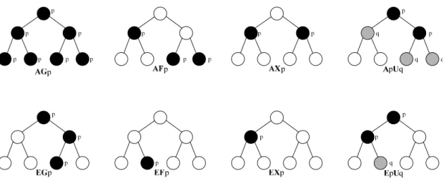
(17) provides language constructs for defining modules and structured data types and for instantiating them.. Finally, the expression part specifies the properties that the user. wants to verify, and the expressions are expressed by computational tree logic (CTL) [23, 24, 25, 33].. 2.3 Computational Tree Logic Computational Tree Logic (CTL) is branching-time logic: its formulas allow for specifying properties that take into account the non-deterministic, branching evolution of a FSM.. The evolution of a FSM from a given state can be described as an infinite. tree, where the nodes are the states of the FSM.. The paths in the tree start at a given. state are the possible alternative evolution of the FSM from that state. The CTL formulas are constructed path qualifiers and temporal operators. Path qualifiers: z. A – “for all the paths”. z. E – “some of the paths”. Temporal operators: z. Xp – “p holds next time”. z. Fp – “p holds sometime in the future”. z. Gp – “p holds globally in the future”. z. pUq – “p holds until q holds”. There are eight CTL operators (AX, AF, AG, ApUq, EX, EF, EG, EpUq) can be used to express properties.. They are illustrated in Figure 2-2.. 7.

(18) Figure 2-2 CTL illustration CTL operators can be nested in an arbitrary way and can be combined using logic operators ( !, &, |, ->, …). For example, AG ( p -> EX q) means that “each occurrence of condition p is followed by at least one path that condition q occurs in the next state.” AG ( p & q -> AF r) means that “for all occurrence of condition p and condition q are followed by condition r occurs at one state for each path finally.” [2, 4, 20]. 2.4 Petri Net 2.4.1 Basic Definition A Petri net C is a four-tuple C = ( P, T, I, O ), where P is a set of places, T is a set of transitions, I is an input function, and O is an output function. P = { p0, p1, p2, ... , pn } is a finite set of places, where n≧0. transitions, where n≧0.. T = { t0, t1, t2, … , tn } is a finite set of. The two sets P and T are disjoint, that is, P∩T =φ.. The. input function I and the output function O record the relationship between places and 8.

(19) transitions. For a transition ti, I(ti) represents the set of the input places of ti and O(ti) represents the set of output places of ti.. In other words, the input function I is a. mapping from a transition ti to a collection of places I(ti), and the output function O is a mapping from a transition ti to a collection of places O(ti). A place pi is an input place of a transition tj if pi ∈ I(tj); pi is an output place of tj if pi ∈ O(tj). A transition could have more than one input places and more than one output places.. A transition also could have no input places or no output places.. A. transition which has no input places means that the transition is always firable and usually used to represent inputs. A transition which has no output places means that firing the transition only eliminates the tokens in its input places and no tokens will be created in any place. A graphical representation of a Petri net is more convenient for illustrating the concepts of Petri net theory and easier for understanding. A Petri net graph consists of two elements, places and transitions.. In a Petri net graph, a place is represented. with a circle ○, and a transition is represented with a rectangle ▌. Places and transitions in a Petri net are connected with arrows.. An arrow directed from a place. to a transition defines the place to be an input place of the transition. An arrow directed from a transition to a place defines the place to be an output place of the transition. Multiple inputs to a transition are expressed by multiple arrows from the input places to the transition. Multiple outputs of a transition are represented by multiple arrows from the transition to multiple output places. However, a place can not connect to a place and a transition can not connect to a transition either. Figure 2-3 is an example of a Petri net graph.. 9.

(20) Figure 2-3 Petri net 1. There are five circles and four rectangles in Figure 2-3. represent places and transitions respectively.. The circles and rectangles. The following is the four-tuple. representation of the Petri net graph in Figure 2-3. C = (P, T, I, O) P = {p0, p1, p2, p3, p4} T = {t0, t1, t2, t3} I(t0) = {p0}. O(t0) = {p1, p2}. I(t1) = {p2 }. O(t1) = {p4}. I(t2) = {p3}. O(t2) = {p0}. I(t3) = {p4}. O(t3) = {p3}. 2.4.2 Marking, State and Reachability. 2.4.2.1 Marking A marking μ is an assignment of tokens to the places of a Petri net.. Tokens in. a Petri net graph are represented with dots ․ in the circles which represent places. The states of a Petri net are determined by the number and distribution of tokens in the Petri net. A Petri net executes by firing transitions. During the execution of a Petri net, the number and distribution of tokens may be changed. A transition can be 10.

(21) fired if each of its input places has at least as many tokens in it as arrows from the place to the transition. When a transition has this condition, we say this transition is enabled (firable).. The tokens in the input places of a transition and make the. transition enable are the enabling tokens of the transition.. Firing a transition will. remove the enabling tokens from its input places and depose into each of its output places one token for each arrow from the transition to the places.. For example, in. Figure 2-4 the tokens in p0 and p3 are the enabling tokens of t0 and t2 respectively. After firing t0, the tokens in p0 will be removed and t0 will depose one token into each of its output places p1 and p2.. The result of firing t0 is shown in Figure 2-5.. Figure 2-4 Petri net 1 state 0. Figure 2-5 Petri net 1 state 1. 2.4.2.2 State The states of a Petri net are defined by markings.. The firing of a transition. indicates a change in the state of the Petri net by changing the marking of the net. Since only enabled transitions can fire, the number of tokens in each place always remains non-negative when a transition is fired. The change in states caused by firing a transition is defined by a change function δ called the next-state function. If a transition ti is enabled, δ(μ, ti) =μ' indicates that firing ti will change the marking from μ to μ'.. When the marking of a Petri net is changed, the state of. the Petri net is changed.. For example, in Figure 2-4, the marking μ= [1 0 0 1 0]T. 11.

(22) After firing t0, the marking will change from μ to μ' = [0 1 1 1 0]T.. 2.4.2.3 Reachability Given a Petri net C = ( P, T, I, O ) and an initial marking μ0, we can execute the Petri net by sequential transition firings.. Firing an enabled transition ti at the initial. marking makes a new marking μ1 =δ(μ0, ti ).. At the new marking μ1, we can. fire any enabled transitions to get a new marking.. Assume that tj is an enabled. transition at μ1, firing tj will get a new marking μ2 =δ(μ1, tj ).. This action can. continue as long as there is at least one enabled transition at the new marking. If the Petri net reaches a marking in which no enabled transition, in other words, there is no transition can be fired, the execution of this Petri net must stop. For a Petri net C = ( P, T, I, O ) with marking μ, a marking μ1 is immediately reachable from μ if there exists a transition ti ∈ T such that δ(μ, ti) =μ1. If a marking μ2 is reachable from μ1 immediately, then we say that μ1 andμ2 are reachable from μ0.. In [1], they define the reachability set R( C, μ) of a Petri net C. with marking μ to be all markings which are reachable from μ.. A marking μ' is in. R( C, μ) if there is at least one sequence of transition firings which will change the marking from μ to μ'.. For example, the initial marking in Figure 2-4 is. μ0 = [1 0 0 1 0]T, after firing the sequence of transitions ( t0, t1 ), we get μ1 = [0 1 1 1 0]T and. μ2 =[0 1 0 0 1]T.. We say that μ1, μ2 ∈ R( C, μ0).. 2.4.3 Matrix Equations There are several approaches to analyze a Petri net, and one of them is based on matrix equations.. Each Petri net could be represented by a transition matrix.. matrix indicates the relationship between places and transitions. 12. The. A transition matrix.

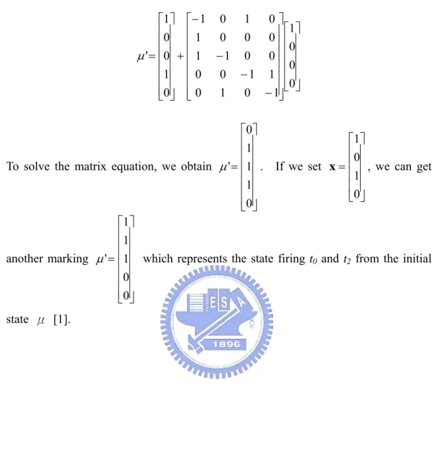
(23) is m (the number of places) rows by n (the number of transitions) columns. Each column represents one transition and records the input places and output places of this transition. The way of recording the relationship of places and transitions is that if there is an arrow directed from a place pi to a transition tj, we put -1 in the ith row by the jth column to mark that pi is an input of tj.. If there are two arrows directed from. pi to tj, then we put -2 in the corresponding position in the matrix and so on.. If an. arrow directed from tj to pk, we put 1 in the kth row by the jth column to mark that pk is an output of tj.. If there are two arrows directed from tj to pk, we put 2 in the. corresponding position in the matrix.. After establishing the transition matrix of a. Petri net, we can represent the Petri net by a matrix equation like the following.. μ' = μ + Ax. (2.1). Here μ is the initial state(marking) of the Petri net; A is the transition matrix records the relationship between places and transitions of the Petri net; x is a transition firing sequence matrix which records the firing times without firing order information of all transitions in the Petri net; μ' is the state(marking) of the Petri net after firing the transitions recorded in x.. Of course, these fired transitions should be. enabled at the state μ. This matrix equation indicates that we can get the next state μ' by adding the product of A and x to μ.. Take Figure 2-4 for example, t0. ⎡1⎤ ⎢0 ⎥ ⎢ ⎥ μ = ⎢0 ⎥ ⎢ ⎥ ⎢1⎥ ⎢⎣0⎥⎦. p0 p1 p2 p3 p4. t1. t2. t3. 0⎤ ⎡− 1 0 1 ⎢1 0 0 0 ⎥⎥ ⎢ A = ⎢ 1 −1 0 0 ⎥ ⎢ ⎥ ⎢ 0 0 −1 1 ⎥ ⎢⎣ 0 1 0 − 1⎥⎦. p0 p1 p2 p3 p4. At the state μ, the enabled transitions are t0 and t2. After t0 fired, as shown in. 13.

(24) Figure 2-5, we can get a new marking by solving the matrix equation 0⎤ ⎡1 ⎤ ⎡ − 1 0 1 ⎢0 ⎥ ⎢ 1 ⎥ ⎡1⎤ 0 0 0 ⎢ ⎥ ⎢ ⎥ ⎢0 ⎥ μ ' = ⎢0 ⎥ + ⎢ 1 − 1 0 0 ⎥ ⎢ ⎥ ⎢ ⎥ ⎢ ⎥ ⎢0 ⎥ 0 − 1 1 ⎥⎢ ⎥ ⎢1 ⎥ ⎢ 0 ⎣0 ⎦ ⎢⎣0⎥⎦ ⎢⎣ 0 1 0 − 1⎥⎦ ⎡0⎤ ⎡1 ⎤ ⎢1 ⎥ ⎢0 ⎥ ⎢ ⎥ To solve the matrix equation, we obtain μ ' = ⎢1⎥ . If we set x = ⎢ ⎥ , we can get ⎢1 ⎥ ⎢ ⎥ ⎢ ⎥ ⎢1 ⎥ ⎣0 ⎦ ⎢⎣0⎥⎦ ⎡1 ⎤ ⎢1 ⎥ ⎢ ⎥ another marking μ ' = ⎢1⎥ which represents the state firing t0 and t2 from the initial ⎢ ⎥ ⎢0 ⎥ ⎢⎣0⎥⎦ state μ [1].. 14.

(25) Chapter 3 Model Checking with Petri Net. For the traditional model checking we told in section 2.1, the verification method is to spread the states from the initial state and then traverse all states to check that if all paths satisfy the properties which the system needs to hold. The drawback of the traditional model checking method is when designs become more and more large and complex, the states need to be traverse will grow dramatically.. Because of this, the. users need to spend more time verifying the designs through state traversing and the time will become considerable.. In order to assist the state traversing based model. checking, we propose a verification method based on Petri net.. Because of the. features of Petri net, the verification method we proposed can reduce the complexity of verifying EX and EF properties and economize on the time users spend verifying. The method we used is to model a FSM in a Petri net and utilize the features of Petri net to reduce the complexity of verification.. In this chapter, we will introduce. the verification flow and the methods of our verification (Petri Net Verification, abbreviate to PNV).. 15.

(26) 3.1 Verification Flow The verification flow of our Petri net based model checking is shown in Figure 3-1. The input of PNV is a SMV code with some constrain we made. The SMV code includes the description of FSMs and properties.. The FSM parts include. signals (inputs and outputs), states and state transition information.. According to the. information, we generate transition matrix and markings and verify the system.. SMV code. Properties (EF, EX). FSM. Marking Generator. FSM to PN Petri net Transition Matrix Generator. Δμ. Transition Matrix Reachability Check. No. True ?. Pass the false properties to SMV. Yes Verification OK. Figure 3-1 Verification flow. When we get a FSM and its properties, first, we transfer the FSM into a corresponding Petri net. Second, we generate the transition matrix based on the Petri net we get before by Transition Matrix Generator. Third, put the properties and 16.

(27) some data from the transition matrix into Marking Generator, we get corresponding markings. system.. After getting the transition matrix and markings, we can start to verify the Because of the limitation of the verification methods, we can only process. EX and EF properties. After verifying, if a property is false, we will pass the property to SMV to verify it again and generate a counterexample. The verification flow is separated into several parts. In the following sections, we will talk about each part step by step. In the first part, we will talk about the transformation from FSM into Petri net. The generation method of transition matrix we have told in section 2.4.3, so we do not talk about it in this chapter. Second, we will discuss how the marking generator generates the corresponding markings based on the properties.. Finally, we will introduce the main verification method of Petri. net based model checking and the limitation of this method.. 3.2 Transformation from FSM into Petri Net 3.2.1 Transformation of Places and Transitions To transform a FSM into a Petri net, we need to know the relation between a FSM and a Petri net. A FSM is composed of the following five parts: z. Q : States. z. Σ: Input alphabet. z. Δ: Output alphabet. z. δ: Q × Σ→Q next-state function. z. Γ: Q → Δ output function. 17.

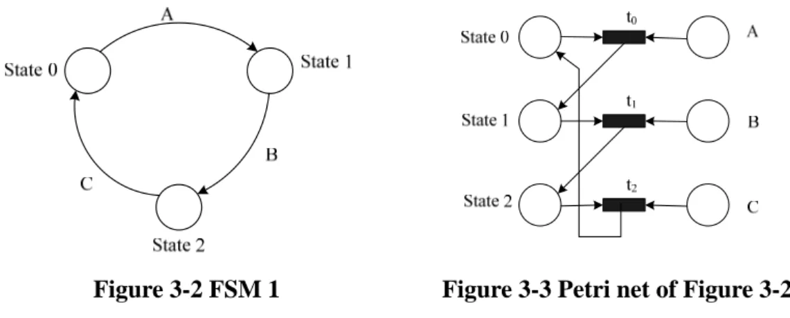
(28) A Petri net is a four-tuple (P, T, I, O).. As a FSM (Q,Σ,Δ,δ,Γ) we define a Petri. net (P, T, I, O) by z. P = Q∪Σ∪Δ. z. T = {tq,σ| q∈Q andσ∈Σ}. z. I(tq,σ) = {q ,σ}. z. O(tq,σ) = {Γ( q )}. According to the illustration above, we could know that all states, inputs, and outputs in a finite state machine are represented with places in a Petri net and all events (arrows) in a state machine are represented by transitions in a Petri net [1].. The rules. of transferring a FSM into a Petri net are:. 1.. Inputs, outputs, and states → places. 2.. Events (arrows) → transitions. 3.. Preconditions → input places. 4.. Post-conditions → output places. The arrows determine the state transitions in a FSM as well as the transitions in a Petri net, so an arrow in a FSM would be transferred into a transition in a Petri net.. The. input places and output places of the transition are the preconditions and post conditions of the arrow in the FSM respectively. After discussing the transformation rules of FSMs and Petri nets, the following are some examples to show the transformation in different situations.. 18.

(29) Figure 3-2 FSM 1. Figure 3-3 Petri net of Figure 3-2. Figure 3-3 is the Petri net transferred from the state machine in Figure 3-2.. In. Figure 3-2, there are three states (State 0, State 1, and State 2) and three signals (A, B, C).. According to the transformation rule 1, there should be three places represent. the states and another three places represent the control signals in the corresponding Petri net.. There are three arrows in the state machine to determine the state. transitions. According to the transformation rule 2, the Petri net needs to have three transitions to represent the three arrows, there are t0, t1, and t2. Finally we connect the places and transitions bottom on the transformation rule 3 and 4 then the Petri net is built. In the above example, we told about the state machine which changes states when control signals are 1(i.e. there is only one value being used for each signal). So there is only one place needs to be built to represent each signal in Petri net. In some state machines, states may change when the control signal is 0 and 1 both.. In. this kind of situation, we should generate two places to represent the two values of the signal. It is illustrated in the following example.. 19.

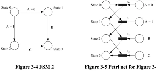
(30) Figure 3-4 FSM 2. Figure 3-5 Petri net for Figure 3-4. In the FSM in Figure 3-4, State 0 may change to State 1 when A = 0 and may change to State 2 when A = 1.. To transfer the FSM into a Petri net in this situation. we should create two places to represent the two values of the signal A. corresponding Petri net is shown in Figure 3-5.. The. The transition t0 controls the state. transition from State 0 to State 1, and t1 controls the state transition from State 0 to State 2. In some cases, we could ignore to transfer some arrows and some values of signals into transitions and places. It is that when a value of a signal which does not control any state transitions, we could ignore the transformation of the value and the arrow. For example, in Figure 3-6, State 0 has a self-loop when A = 0. Assume the initial state is State 0, and A = 0, the state is still at State 0 until A = 1. This FSM could have the same behavior even if we ignore the transformation of the arrow controlled by signal A = 0.. Because A = 0 does not determine any state transitions.. Figure 3-6 FSM 4. 20.

(31) But in some other case, we still generate transitions and places even if the arrows and signals do not determine any state transitions.. An example is shown in section 5.2.. From the three examples above, we can observe that in some situations we transfer one signal into one place, but in other situations we transfer one signal into two places. Theoretically speaking, we should always transfer a signal in a FSM into places based on its values. In other words, when a signal A can be 0 and 1, we should generate two places to represent A = 0 and A = 1. But some values of signals do not control any state transitions. For example, the value 0 of the signal A in Figure 3-2 do not control any state changes in the FSM, we don’t need to generate a place to represent A = 0 and the transition controlled by A = 0 either.. It is no effect. that we do not generate the place A = 0 and the transition in the corresponding Petri net.. Summarily speaking, when there are any arrows which do not determine state. transitions, we could ignore the transformations of the arrows.. We only transfer the. signals and arrows which are used into places and transitions respectively.. By doing. this, we could make the corresponding Petri net more concise and the transition matrix of the Petri net smaller. There is a special kind of transitions which do not have input places.. The. transitions are firable all the time and usually connected in front of inputs to provide the input places tokens. When we meet a situation that we don’t know how many tokens we have to assign to an input signal (e.g. clk), we put an input transition in front of the place to generate tokens to the signal.. 21.

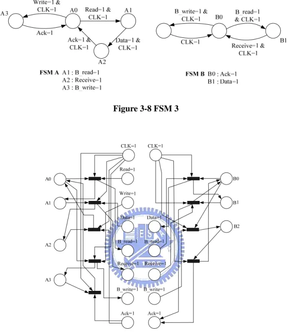
(32) Figure 3-7 Petri net 1 In Figure 3-7, t3 to t5 are input transitions, they provide tokens to the inputs A, B and C respectively.. 3.2.2 Transformation of Multiple Modules When a system consists of more than one module and these modules communicate with each other, we could transfer the modules into a Petri net as the following steps.. 1.. Transfer each module into a Petri net individually. 2.. Merge the same places which are used in different Petri nets.. In Figure 3-8, it is a simple example to model bus communication protocol. is master and FSM B is slave. writing.. FSM A. This system models the behavior of reading and. The initial states of the two state machines are A0 and B0.. 22.

(33) Figure 3-8 FSM 3. Figure 3-9 Petri net of Figure 3-6. 23.

(34) Figure 3-10 Petri net combine from Figure 3-8. According to the rules we told above, the first step is to transfer the two state machines into Petri nets individually. The transformation result is shown in Figure 3-9.. The left Petri net is transferred from FSM A and the right one is transferred. from FSM B.. Because of the cooperation of these two FSMs, there are many places. which appear in both Petri nets. Then we merge the same places of the two Petri nets. After merging some places of the two Petri nets, we get one Petri net shown in Figure 3-10. This Petri net is the result transferred from the system in Figure 3-8.. 3.3 Marking Generator The function of marking generator is to transfer the properties into corresponding markings.. Markings represent the states of Petri nets. A property is written as. 24.

(35) “O1 (starting state → O2 (ending state))”, O1 and O2 are CTL operators.. The. starting state and ending state here can be mapping to μ and μ' in equation 2.1 respectively. To transfer a state into a marking, we put one token in each place which represents the state or signal mentioned in the state description.. The. expression of a token in matrix equation of a Petri net is putting 1 in the position which represents the place.. In order to make the verification process convenient, we. rewrite equation 2.1 as. Δμ = Ax. where Δμ = μ' – μ.. (3.1). The actual information we need is Δμ. So, the rules. of transferring the starting state and the ending state into Δμ are. 1.. In a marking matrix (μ), we put 1 in each place which represents the state mentioned in the starting state.. 2.. In another marking matrix (μ'), we put 1 in each place which represents the state mentioned in the ending state.. 3.. Through subtracting μ from μ', we get Δμ.. To simplify the transformation steps, we change the way we do above. First we fill the matrix Δμ with 0. Then we add -1 instead of 1 in each place which represents the state mentioned in the starting state in a marking matrix and add 1 in each place which represents the state mentioned in the ending state in the same matrix. doing this, we can directly get the matrix Δμ.. 25. By.

(36) 3.4 Reachability Checking We have introduced in section 2.4.3 that a Petri net could be analyzed by a matrix equation and the equation could be express as equation 3.1. According to linear algebra theorem [34], a linear system Ax = b is consistent if and only if the rank of A is equal to the rank of (A | b), where (A | b) is the augmented matrix.. For. example, from Figure 2-4 and 2-5 we can get 1 0⎤ ⎡− 1 0 ⎢1 0 0 0 ⎥⎥ ⎢ A = ⎢ 1 −1 0 0⎥ ⎢ ⎥ 0 −1 1 ⎥ ⎢0 ⎢⎣ 0 1 0 − 1⎥⎦. ⎡0⎤ ⎡1⎤ ⎡− 1⎤ ⎢1⎥ ⎢0⎥ ⎢ 1 ⎥ ⎢ ⎥ ⎢ ⎥ ⎢ ⎥ Δμ = ⎢1⎥ − ⎢0⎥ = ⎢ 1 ⎥ ⎢ ⎥ ⎢ ⎥ ⎢ ⎥ ⎢1⎥ ⎢1⎥ ⎢ 0 ⎥ ⎢⎣0⎥⎦ ⎢⎣0⎥⎦ ⎢⎣ 0 ⎥⎦. ⎡− 1 0 1 0 ⎢ 0 0 0 ⎢1 ( A | Δμ ) = ⎢ 1 − 1 0 0 ⎢ 0 −1 1 ⎢0 ⎢0 1 0 −1 ⎣. − 1⎤ ⎥ 1⎥ 1⎥ ⎥ 0⎥ 0 ⎥⎦. If the state in Figure 2-5 is reached from the state in Figure 2-4, the rank of A will be the same as the rank of matrix (A |Δμ).. To evaluate the ranks of A and (A |Δμ),. we use Gaussian elimination [34] to reduce the two matrices into reduced row echelon form and normalize the lead variables of each row. After going through the steps, we get two matrices in row echelon form like the following. ⎡1 ⎢0 ⎢ Reduced A = ⎢0 ⎢ ⎢0 ⎢⎣0. 0 1 0 0 0. 0 0 1 0 0. ⎡1 0⎤ ⎢ ⎥ 0⎥ ⎢0 0⎥ and reduced ( A | Δμ ) = ⎢0 ⎢ ⎥ 1⎥ ⎢0 ⎢0 0⎥⎦ ⎣. 0 1 0 0 0. 0 0 1 0 0. 0 0 0 1 0. 1⎤ ⎥ 0⎥ 0⎥ ⎥ 0⎥ 0⎥⎦. The rank of A = 4 and the rank of (A |Δμ) = 4. This linear system is consistent and we can get solutions of the transitions directly from the most right column. The ⎡1 ⎤ ⎢0 ⎥ solution of the system is x = ⎢ ⎥ . This solution means that we can reach the state ⎢0 ⎥ ⎢ ⎥ ⎣0 ⎦ of the Petri net in Figure 2-5 from the state in Figure 2-4 by firing the transition t0 one 26.

(37) time. Through this linear algebra method above, we can only know that this system has a solution or not.. This condition can make us apply it to check EX and EF. properties. Because as long as we can find any situation that makes the system satisfies the property which is EX or EF, we can say that the system satisfies the property.. The other kinds of properties (AX, AF, AG…) may not have many. advantages to be verified by this method because that to verify a system which satisfies these kinds of properties (AX, AF, AG…) needs to be proved that more than one situation or all situations of the system which satisfy the properties. So the main point in this paper is the methods to speed up verifying EF and EX properties with modeling a FSM in Petri net. Before we start to solve the solutions of a matrix equation, we need to know the ranks of the matrices. When the ranks of A and (A |Δμ) are equal, we can only know that the linear system has solutions. When the ranks of the matrices are equal to the number of its transitions, we can get a unique solution of the system.. When. the rank of the matrix is less than the number of its transitions, there are infinite solutions of the equation. The solution of a matrix equation is a set of the firing times of transitions in a Petri net, and the firing times must be integers and greater than 0. Proving the equation is consistent is not enough to confirm that the system satisfies the property. We need to do some other process to ensure that there is at least one solution exists and satisfies the following two rules (Firing Times Rules).. 1.. The values of the firing times should be equal or greater than 0.. 2.. All the firing times should be integers.. 27.

(38) In other words, when the ranks are equal to the number of transitions, we have to solve the solution and check if the solution conform the Firing Times Rules; when the ranks are less than the number of transitions, we also need to ensure that there exists at least one solution satisfies Firing Times Rules.. 3.4.1 Ranks are Equal to the No. of Transitions When the ranks of a matrix equation are equal to the number of its transitions, we can use the method we told above to verify the linear system and confirm that this system has at least one solution then check if the solution satisfies Firing Times Rules. To verify an EF property we only need to solve the solution and check if the solution satisfies the Firing Times Rules. If the answer is YES and we can say that the EF property is true. To verify an EX property we not only need to solve the solution and check if the solution satisfies the Firing Times Rules but also need to check one more rule which is: z. All fired transitions should not have any correlation with each other.. Proof: 1. For a FSM, there is only one state which the state machine is staying at. So in a Petri net transferred from a FSM, there is only one place which represents one of the states with a token in it. 2. For each transition, one of its input places must be a state place. In other words, firing a transition must cause a state transition. Because of the two reasons, for a Petri net transferred from only one state machine, when we solve the firing sequence which has more than one transition. 28.

(39) fired, the fired transitions must have causal relation with each other. For a Petri net transferred from more than one FSM, the Petri net can fire more than one transition at one time.. But the fired transitions should not have casual relation. with each other, too. When a firing sequence in which the fired transitions have casual relation with each other, the final state must be not the next state of the initial state.. The method of checking the rule is that the output places of each fired transition should not be other fired transition’s input places.. When the fired transitions do not. have any casual relation with each other, we can ensure that the final state is the next state of the initial state. If there is a fired transition its input places are other fired transition’s output places, it means that there is causal relationship between these two transitions. State transition causing by firing two successive transitions may not satisfy EX properties, i.e. the ending state is not the next state of the beginning state. The verification flow of ranks = NO. of transitions is shown in Figure 3-11.. Figure 3-11 Flow of ranks = NO. of transition 29.

(40) 3.4.2 Ranks are Less Than the No. of Transitions The cause of that the ranks are less than the number of transitions is that the FSM has loops and when we transfer the state machine into a Petri net we generate transitions without input places and the output places are the control signals. For example, in Figure 3-12(a), the state machine has a loop and three control signals. We transfer the state machine into a Petri net in figure 3-12(b) and generate three transitions (t3, t4, t5) without input places to put tokens into signal places.. (a). (b). (c) (d) Figure 3-12 Example of the ranks < NO. of transitions In this example, we set a property: “AG ( S0 -> EF (S2))” to the FSM. The reduced matrix is shown in Figure 3-12(d). In this kind situation, the ranks will be less than the number of transitions and we can adjust some transitions to make the Petri net go through the loop one time of more. In this example we can adjust the firing times of t5. In Figure 3-12(d), if we set t5 = 0, the solution of the matrix equation will be (1, 1, 30.

(41) 0, 1, 1, 0) and the state transition process is S0 → S1 → S2; if we set t5 = 1, the solution will be (2, 2, 1, 2, 2, 1) and the state transition process is S0 → S1 → S2 → S0 → S1 → S2.. According to the illustration above, when the ranks of a matrix equation are less than the number of its transitions, we have to use some other methods to confirm that there is at least one solution satisfies the properties and the Firing Times Rules. For EF properties, first we eliminate the matrix (A |Δμ) into reduced row echelon form. Then we check each coefficient in each row to comprehend if the matrix obeys the following two rules.. 1.. For each row, when the signs of the coefficients in the A part are the same, the sign of the value in Δμ column must be also the same as the signs.. 2.. When there are positive and negative coefficients in the A part, we do not care the sign of the value in Δμ column.. When the matrix (A |Δμ) satisfies the two rules above, we can say that this matrix equation could be found a solution set which satisfies the Firing Times Rules. The following is an example to illustrate the two rules above.. Figure 3-13 (a). 31.

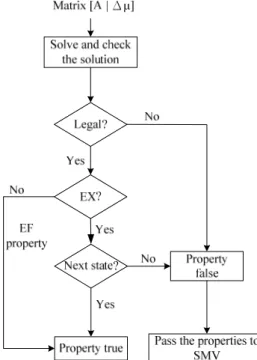
(42) (b) Figure 3-13 Example of illustrating EF properties judging rules. In Figure 3-13(a) row 0, the coefficients in the A part are zero except column t0. The sign of (0, t0) is positive and it is the same as (0, Δμ). So we can find a legal solution of t0.. In row 1, there are three non-zero coefficients and they are all. positive, and the value (1, Δμ) is also positive.. We can find solutions of t1, t6, t9. such that satisfy the equation and the Firing Times Rules like (t1, t6, t9) = (1, 0, 0). When there are positive and negative coefficients in a row in the A part, it means that there is at least one loop in this system and we can adjust some transitions to change the firing times of other transitions. So for one row, no matter what the sign of column Δμ is, we always can find a solution set that satisfies the equation when there are positive and negative coefficients in the A part. In Figure 3-13(b), the coefficient in row 0 column t0 is positive but Δμ is negative. They have different signs and the solution of t0 must be -1, it violates the Firing Times Rules. In row 1, there are three positive coefficients in the A part but the value of Δμ is negative. We can not find any solutions of (t1, t6, t9) which are positive integers and satisfy the equation. For EX properties, we always need to solve the solution to verify it. Because even though the matrix equation has a solution which satisfies Firing Times Rules, we also need to check if the solution satisfies next state property. So, when we meet an 32.

(43) EX property and the ranks of the matrix equation are less than its number of transitions, we can not get a solution and also can not verify EX properties at this kind of situation. The verification flow of ranks < NO. of transitions is shown in Figure 3-14. Matrix [A | Δμ]. No. Yes. EF?. EX properties. EF properties Check if there are any legal solutions. Can not verify. No. Property false. Exist? Yes. Pass the properties to SMV. Property true. Figure 3-14 Flow of ranks < NO. of transitions. 3.4.3 Summary According to the illustration in the two section above, we could make a brief summary that when we find the ranks of the matrices A and (A |Δμ) of a system are equal and the same as the number of its transitions, we will solve the matrix equation and check if the solution tallies with Firing Times Rules. When the ranks are equal and the solution satisfies the rules, we will show that the property is true. When we find that the ranks of the matrices are equal but they are less than the number of its transitions, if the property is EF, we will check if the matrix has solutions satisfies Firing Times Rules. When the property is EX, we can not verify it and will pass the property to SMV directly.. When we find that the ranks of the two matrices are not 33.

(44) equal, we will directly show that the property is false and pass the property to SMV. The total verification flow is shown in Figure 3-15.. Figure 3-15 PNV software verification flow. 34.

(45) Chapter 4 Implementation. In this section, we will discuss the implementation of PNV for each block in Figure 3-1.. 4.1 Input Coding Rules The input data of PNV is a SMV code which should obey the coding rules we made. The coding rules are made for us to transfer FSM descriptions into a Petri net structure more easily and conveniently. The codes which obey the coding rules are still readable by SMV model checker. The coding rules are. 1.. A signal which controls two state transitions should be named starting with “_”, e.g. “_enable”.. 2.. In the input SMV code, each symbol, signal name, and keyword should be separated by a blank space.. 3.. The properties should be described completely including the states and the values of signals.. 4.. Adding “--” at the end of the signal transition descriptions which do not need to be transferred into transition in Petri net. 35.

(46) The first rule is made for PNV to recognize which signal needs to be transferred into two places. The second rule is made for PNV to read the input SMV code easily. The purpose we make the third rule is to make marking generator generate markings easily. The fourth rule can make a Petri net and its transition matrix smaller in some situation. Even if we don’t allow the fourth rule, the codes are still readable for PNV. Figure 4-1 is a simple example of SMV code which obeys the coding rules above.. Figure 4-1 SMV code of counter. Figure 4-1 is a finite state machine of a counter. From line 1 to line 3 and from line 17 to line 20 are the definitional part. Line 1 declares a module called counter and enable is its input. Line 3 declares the state of the counter which has eight values from 0 to 7. From line 4 to line 16 are the structural part. Line 5 defines that the initial value of state is 0. From line 6 to line 16 define the state transitions of counter. Line 7 describes that when enable = 0 and state = 0, the next state is still 0.. We don’t. need to generate any transition in Petri net for this description. So, according to the. 36.

(47) 4th coding rule, we add “--” at the end of line 7. Line 17 is main module in which the designer defines the connections of all sub-modules. From line 21 to line 24 are the expression part. Line 22 and line 24 are the properties of this system. The modules before main module are sub-modules which are used in main module. The descriptions in main module connect the whole sub-modules together and define properties.. 4.2 Data Structure of PNV The work of PNV is to transfer a SMV code into Petri net structure and to generate the transition matrix then verify it. Figure 4-2 is the data structure of a Petri net built by PNV.. Figure 4-2 Data structure of PNV. There are three objects, Module, Place, and Transition, in the structure. For each module, there are three elements, a place vector, a transition vector, and a string, in it. 37.

(48) Each place has a string to represent its name. Each transition has two place vectors, one is to store the input places of the transition and the other is to store the output places of the transition [35]. The first step of building a Petri net is to generate modules.. When PNV reads. the keyword, MODULE, PNV pushes a new module which is named as the word after MODULE in the SMV code into the module vector. After creating a new module, PNV continues to build the places and transitions of this module according to the declarations in VAR part and ASSIGN part respectively. PNV creates one or two places to represent a signal which is declared as a Boolean signal. When there is a signal which is a set of signals like states, PNV creates places according to the number of signals in the set. For example, in Figure 4-1, PNV may push a module named “counter” in the module vector first and then push one place to represent the input signal, enable, and eight places to represent the signal, state (a set of signals), in the place vector which belongs to counter. When PNV reads a signal which is starting with “_” (coding rule 1st), PNV pushes two places into the place vector to represent the two values of the signal. After generating all places, the next step is to build the connections of places and transitions.. The descriptions in the ASSIGN parts in a SMV code express the. relationship of places and transitions. PNV builds the connections of places and transitions based on the descriptions. In Figure 4-1 line 8, when PNV reads this description, PNV knows that there is a transition which has two input places, state=0 and enable=1, and one output place, state=1. Then PNV pushes these I/O data into the transition vector. After pushing all transitions into the transition vector, a module is built completely. Then PNV continues to build the following modules using the same methods. After building all sub-modules, the last module must be main module. Main 38.

(49) module is a module which composes the sub-modules to become a complete system. The work of main module is to build the interconnections of the sub-modules included in main module. Figure 4-3 is an example that there are two sub-modules, fsm_a and fsm_b, in this system.. Figure 4-3 SMV code. The main module includes two sub-modules and declares two new signals in its VAR part.. The two sub-modules included in main module are named FA and FB. respectively. The signals in FA and FB will be named starting with “FA.” and “FB.” respectively. It is to mark the origin of the signals in main module. Line 24 and 25 in Figure 4-3 are ports mapping of the two sub-modules. When PNV reads line 24, PNV copies the places and transitions from the module fsm_a to main module. After copying the places and transitions, PNV changes the names of the places into starting with “FA.” and changes the names of the input signals from their original 39.

(50) names into the corresponding names that connect to the input ports. For example, in Figure 4-3 line 24, PNV copies the places from fsm_a and changes the names. Besides the input signals, all places’ names would be changed starting with “FA.”. But the input signals, _BWRITE, DSELAPB and PD, will be changed as _BW, DSEL and FB.PD respectively. _BW and DSEL are input signals from outside and FB.PD is an inner signal of the system from fsm_b. After processing the VAR part of main module, the whole system is built completely. After building a whole Petri net structure, the following step is to generate the matrix.. Because PNV stores places and transitions in the place vector and the. transition vector respectively in main module, we can easily know that how many places and transitions in this system. The number of rows is the number of places of the system and the number of columns is the number of transitions. We get these data from the two vectors and generate a corresponding size matrix. Then PNV fills the matrix according to the illustration we told in section 2.4.3. After doing so, the matrix is accomplished.. 4.3 Property to Marking To verify a system represented with Petri net, we need to transfer its properties into markings. From the above works, each place stored in the place vector has an index to locate where it stored in the vector.. We use the indexes to locate the. positions of the places and create an n (the number of places) by 1 matrix to store the marking of each property. The methods of transfer a property into a marking is illustrated in section 2.4.2 and section 3.3. The information we need to verify is Δμ = μ' – μ. A property description is beginning from its starting state and 40.

(51) finishing at the ending state. The starting state is μ and the ending state is μ'. According to the transformation methods in section 3.3, we can directly compose the generation of μ and μ' by adding 1 in the places of the ending state and adding -1 in the states in the starting state.. So when PNV reads a property, it adds a. corresponding number in each space in the marking matrix. For example, in Figure 4-1 the first property in line 22 describes that the starting state is en=1 and cnt.state=0, PNV adds -1 in the spaces which represent en=1 and cnt.state=0 and adds 1 in the spaces which represents cnt.state=7. Those spaces represent other places are still 0. Figure 4-4 is the transition matrix and the first marking in Figure 4-1.. Figure 4-4 Transition matrix. 4.4 Verification Core After the collection of markings and transition matrix, PNV can start to verify the system with the methods we have told in section 3.4.. Assuming that the. transition matrix is an m by n matrix and the markings are m by 1 matrix. First, PNV creates a new empty matrix and copy the transition matrix into the matrix and. 41.

(52) then do Gaussian elimination to evaluate the rank of the transition matrix. Second, PNV copies the transition matrix into the new matrix again and copies the marking into the next column of the transition matrix, the matrix becomes (A |Δμ). Then PNV starts to evaluate the rank of the (A |Δμ) matrix.. When the two ranks are. unequal, this matrix equation does not have solutions. PNV will pass the property to SMV to verify it again and generate a counterexample. When the two ranks are equal and the same as the number of its transitions, PNV will solve the solutions of the equation and check if all solutions satisfy Firing Times Rules. When PNV gets an EX property, there is one more rule should be checked. It is that the fired transitions in the solution should not have causality. The reasons we have told in section 3.4.2. When the property is EF and the ranks are equal but less than the number of its transitions, PNV will check if the equation has a solution satisfies Firing Times Rules. When the property is EX and the ranks are equal but less than the number of its transitions, PNV can not verify the property and will pass the property to SMV.. 4.4.1 Elimination Methods The elimination method of PNV is based on Gaussian elimination and some special methods.. The methods are devised according to the characteristic of. transition matrices to simplify the computational complexity of the elimination process. A transition matrix of a Petri net has a characteristic that the most values in the matrix are zero. For each column, only the rows which represent the places connect to this transition have non-zero values.. For each row, only the columns which. represent the transitions connect to this place have non-zero values. In other words, 42.

(53) in a transition matrix, the most values are zero and the second most values are 1 or -1. The causes of this characteristic are that for each row, the non-zero columns are the transitions connected with the place. For a place, especially state place, there are not many transitions connect with it. This characteristic means we can utilize some specific methods to eliminate a transition matrix with fewer steps than using general Gaussian elimination. During generating a transition matrix, we would put the state places together to make the characteristic more obvious. By doing so, the work of elimination may be reduced outstandingly. One of the methods we devise is that when we find one row with zero lead value, we can ignore this row in the elimination step.. In other words, we check the. representative value and decide if we need to eliminate this row.. When the. representative value is not zero, we have to eliminate it, but if the value is zero, we can skip the row. Though checking the representative value, we can save the work of eliminating unnecessary rows. According to this method, we can avoid some unnecessary calculation.. So, we can say that the method devised from the. characteristic of a transition matrix can make us more easily and quickly eliminate the transition matrices. Because of the characteristic of a transition matrix, there is another method could be used to simplify the complexity of elimination. We check the values in the pivotal row and memorize the columns of the non-zero values. When we start to eliminate other rows, we can only calculate the non-zero columns and skip the other columns which are zero. By using this method, we can reduce the calculation when we meet a row which needs to be eliminated. According to the methods above, the first step of elimination is to find out a non-zero value in the first column to be the pivotal row.. When the pivotal row is not. the first row, we have to exchange the pivotal row with the first row. Then we check 43.

(54) all values in the pivotal row and record the column indexes of the non-zero values. The next step is to eliminate the first column.. We will check the values in the first. column and eliminate the non-zero rows. The following is an example illustrating the steps we mentioned above.. (a). (b). (c) Figure 4-5 Eliminating example. Figure 4-5(a) is a transition matrix. For the first column, the (0, 0) position is zero, so row 0 can not be the pivotal row.. We continue to check (1, 0) and find that. it is a non-zero value, so we exchange row 0 and row 1 to become the matrix shown in Figure 4-5(b). After deciding the pivotal row, we start to check the items in the pivotal row and record the indexes of non-zero values. We find that column 0 and column 7 are not zero and we record the indexes 0 and 7. Then we start to eliminate the non-zero values in column 0 and only calculate the columns we have recorded. 44.

(55) In this example, we can eliminate the first column through four times of calculation with our methods instead of use full Gaussian elimination with sixty-four times of calculation. For an m by n matrix, we assume that m and n are the same order and m = n + k. To find out the first pivotal row and exchange it to the first row, we have to check column 0 m times in the worse case and do 3n times to exchange the two rows. To find the second pivotal row, we have to check (m - 1) times and exchange 3(n - 1) times. The above operations we have to do for a matrix are. [m + 3n] + [(m - 1) + 3(n - 1)] +... = [(n + k) + 3n] + [(n + k - 1) + 3(n - 1)] +… =. n. ∑ (i + k ) + 3i i =1. =. n. ∑ 4i + k i =1. = 2n (n + 1) + kn = 2n2 + (2 + k) n. The computational complexity of finding the pivotal row and exchanging it to the right position is O(n2 ). To eliminate the first column, we have to check (m – 1) rows to figure out which rows need to be eliminated and we assume that there are ci rows need to be eliminated. Before we start to eliminate, we need to check the values in the pivotal row and it cost n operations. After checking the pivotal row, we find out that there are di non-zero values. So the number of calculation we need to do is ci * di. The total operations we have to do for eliminating a matrix into reduced row echelon form are. 45.

(56) [n + (m - 1) + c1 * d1] + [(n - 1) + (m - 1) + c2 * d2] +… = [n + (n + k - 1) + c1 * d1] + [(n - 1) + (n + k - 1) + c2 * d2] +… =. n. ∑ i + (i + k − 1) + c * d i. i =1. =. i. n. ∑ 2i + (k − 1) + c * d i. i =1. = n (n + 1) + (k - 1) n +. i n. ∑c * d i =1. = n2 + kn +. ∑c * d. n. ∑c * d i =1. i. i. n. i =1. The order of. i. i. i. i. term is about n.. The computational complexity of the. elimination step is O(n2 ). After the elimination step, we get a matrix in reduced row echelon form.. When the rank of the matrix is equal to its transition number, we can. get the firing times of each transition without more action. An example is shown in Figure 4-6, the matrix is in reduced row echelon form and the rank is the same as its transition number, so we can get the solutions of t0 to t5 are a to f without back substitution.. Summarily, the total computational complexity of our elimination. process is O(n2 ) and its order is lower than the computational complexity of original Gaussian elimination O(n3 ). The methods we use to eliminate a transition matrix can reduce the order of computational complexity from O(n3 ) to O(n2 ).. t0 t1 t2 t3 t4 t5 Δμ 0 1 2 3 4 5. 1 0 0 0 0 0. 0 1 0 0 0 0. 0 0 1 0 0 0. 0 0 0 1 0 0. 0 0 0 0 1 0. 0 0 0 0 0 1. a b c d e f. Figure 4-6 Reduced row echelon form. 46.

(57) Chapter 5 Experimental Results. In this chapter, we will use PNV to verify five examples and interpret the rules we mentioned above. The simulation environment of the following examples is: “OS: Windows XP, CUP: AMD 3000+, RAM: 1GB.”. 5.1 Counter Figure 5-1 is a finite state machine of a four-state counter. The initial state of the FSM is s0.. Figure 5-1 FSM of counter. Figure 5-2 is the Petri net graph and its transition matrix of the counter. In Figure 47.

(58) 5-2(a), there are two places used to represent the reset signal. It is because that state transitions should always happened when reset = 0. So we need two places to indicate reset = 1 and reset = 0 as shown in Figure 5-2(a). The transitions t0 to t3 are working for state transition, t4 to t7 are working for reset, and t8 to t10 are for input signals. The transitions t0 to t3 always need one input place which is reset = 0 to ensure that the system is not being reset.. (a). (b). Figure 5-2 Petri net of the counter. The property of this Petri net we set is “AG (state=0 -> EF (state=3))”.. This. property means that there is at least one path starting from state = 0 and finally ending at state = 3. We verify this property by SMV and PNV respectively. Figure 5-3 is the verification result generated by PNV verbose mode.. Figure 5-3(a) shows the. places and the transitions generated by PNV. The first part in Figure 5-3(b) shows the transition matrix of the Petri net, the second part shows the matrix after being eliminated and the rank of this matrix, the third part shows the property and the corresponding marking, the fourth part shows the result of eliminated (A |Δμ), and. 48.

(59) the final part shows the verification result of the property and time cost. There is a brief mode of PNV shown in Figure 5-4, this mode only shows the result and time cost of the properties and it is faster than verbose mode.. Figure 5-5 is the. verification result generated by SMV.. (a). (b). Figure 5-3 Verification result of counter with PNV verbose mode. 49.

(60) Figure 5-4 Verification result of counter with PNV brief mode. Figure 5-5 Verification result of counter with SMV SMV Time (ms) Memory (KB). PNV. Processor. Total. Verbose. Brief. 16. 300.699. 13.0455. 1.00963. 1184. 1940. Table 5-1 Time cost of SMV and PNV for counter In this example, the rank of A and (A |Δμ) are less than the number of transitions.. We can not get an exact solution, so we verify this design by the. methods illustrated in section 3.4.2. The time costs of SMV and PNV are shown in Table 5-1. The SMV processor time is clocked by SMV and we don’t know what action included in this time interval and the accuracy is lower than the timer used by PNV.. So we add another timer to. clock the time cost of SMV, the result is shown in SMV Total. This result includes all action of SMV and its clocking condition is the same as PNV.. Adding another. timer to clock SMV makes us more convenient to compare the time costs of SMV and PNV.. From Table 5-1 PNV part, we could notice that the most time cost by PNV is 50.

(61) to print out the result. The processing time depends on the status of CPU, so the time cost of each processing may not be equal; even so, we still can find that the time which is shown in Table 5-1 costs of PNV are fewer than the time costs of SMV, especially at PNV brief mode.. 5.2 Greatest Common Divisor In this section, we will show an example about greatest common divisor (GCD) and verify it by SMV and PNV. Figure 5-6 is the FSM of GCD. The state s0 is idle mode, this machine starts when the start signal = 1 and the state transfers to s1. At s1, the machine transfers its state according to the inputs, u > v, u < v, and u = v. The state will transfer to s2 and s3 when u > v and u < v respectively. At these two states, the system will subtract the smaller number from the larger one then send the answer and the smaller number to a comparator.. The comparator will identify which. number is larger and send the result (u > v, u < v, or u = v) to GCD system.. When. the two numbers are equal, the state will transfer to s4 and the process is finished. The final number is the GCD of the original u and v.. 51.

(62) Figure 5-6 FSM of GCD. (a). (b) Figure 5-7 Verification result of GCD with PNV verbose mode 52.