應用整數線性規劃達成架構層級合成上 最佳化通道與暫存器配置之技術

國 立 交 通 大 學

電子工程學系 電子研究所碩士班

碩 士 論 文

應用整數線性規劃達成架構層級合成上

最佳化通道與暫存器配置之技術

Optimal Channel and Register Allocation in

Architecture Level Synthesis Using ILP

研 究 生：黃維聖

指導教授：黃俊達 博士

應用整數線性規劃達成架構層級合成上

最佳化通道與暫存器配置之技術

Optimal Channel and Register Allocation in

Architecture Level Synthesis Using ILP

研 究 生：黃 維 聖 Student: Wei-Sheng Huang

指導教授：黃 俊 達 博士 Advisor: Dr. Juinn-Dar Huang

國立交通大學

電子工程學系 電子研究所碩士班

碩士論文

A Thesis

Submitted to Department of Electronics Engineering & Institute of Electronics College of Electrical and Computer Engineering

National Chiao Tung University in Partial Fulfillment of the Requirements

for the Degree of Master in

Electronics Engineering & Institute of Electronics

Augest 2006

Hsinchu, Taiwan, Republic of China

應用整數線性規劃達成架構層級合成上

最佳化通道與暫存器配置之技術

研究生：黃 維 聖 指導教授：黃 俊 達 博士 國立交通大學 電子工程學系 電子研究所碩士班

摘 要

在深次微米科技裡，連線的延遲已經不再能被忽略。而且隨著製程的日益進步，更 漸漸地主導了系統的時間延遲。規律分散式暫存器架構著眼在這個問題上。其相對的 合成流程分散了暫存器並且利用實體區域化的特性來改善整個系統的時間延遲。然 而，多出來的溝通代價，包含連線和暫存器卻限制了應用程式的規模。我們針對這個 問題並且提出了所謂“在架構合成層次上通道與暫存器配置”的問題。輸入這個問題的 是經過排程而且已經指定運算單元的資料流程圖、運算單元的擺置和代表目標架構的 拓樸圖。目標是得到一個配置，它將每一個週期的所有傳輸資料對應到可使用的通道 和暫存器上同時降低溝通的資源。除此之外，我們提出了這個問題正式的模型。藉由 比重分配過的目標函式，我們能使用處理線性規劃的程式來得到最佳解。除此之外， 由捕捉到每一個基本傳輸行為的好處，我們延伸了這一個模型，以利用後製的方式使 他得到更進一步的改進並且模擬了雙向的通道。在實驗的結果裡，相較於之前僅僅使 用專屬溝通的方法，我們所提出的線性規劃模型分別改善了平均 58% 和 35% 在連線 和暫存器的使用上。就算和使用了管線連線而且執行了傳輸排程的方法比較，我們提 出的方法也擁有分別為 46% 和 54% 的改善在連線和暫存器的使用上。

Optimal Channel and Register Allocation in

Architecture Level Synthesis Using ILP

Student: Wei-Sheng Huang Advisor: Dr. Juinn-Dar Huang

Department of Electronics Engineering & Institute of Electronics National Chiao Tung University

Abstract

In deep submicron technology, the wiring delay has no longer been trivial and dominated the system latency gradually. The regular distributed register architecture is proposed to resolve this problem. The corresponding synthesis flow partitions the registers and exploits the physical locality to improve the system latency. However, it introduces the extra interconnection overhead, which includes wires and registers, and limits the scale of applications. We address this problem and formulate it as channel and register allocation in architecture level synthesis problem. The inputs are the scheduled and bound DFG, placed FUs and topology information of the target architecture. The goal is to get the assignment which maps all transferred data to available channels and registers at each cycle while minimizing the interconnection resource at the same time. Besides, we propose a formal model for this problem. With the weighted objective function, we can get the optimal solution through an ILP solver. Furthermore, due to the benefit of capturing the basic transfer behavior in our formulation, we also extend the model to get the further improvement and model the bi-directional channel through post processing. According to the experimental results, our proposed ILP method improves 58% and 35% on average in terms of usage on wires and registers compared to the previous method, which uses dedicated interconnections only. Even compared to another one, which uses pipelined wires and performs transfer scheduling, our method gets 46% and 54% improvement in terms of the usage on wires and registers.

誌 謝

首先，我要感謝我的指導教授-黃俊達老師：在兩年的碩士生涯裡，讓我在研究領域 上自由發揮。老師總是用支持與鼓勵的態度，包容我的創意且讓我在學術的領域裡不斷 進步。這份感激的心，是無法用簡單的三言兩語帶過的。 感謝我的口試委員，交大電子—周景揚教授，清大資工—林永隆教授，清大資工— 黃婷婷教授：在百忙之中蒞臨指導。你們寶貴的意見讓我對問題有了新的認識及啟發， 更提供了我研究上再進步的方向。 也要感謝我一群實驗室的好伙伴，士祐、宏光、翊展、孝恩、詠翔、學弟們以及所 有曾經在一起的同學：我們互相砥礪切磋，讓我在學習的道路上不孤單。我永遠不會忘 記這一段日子，相信我們會是一輩子的好朋友。 最後我感謝我的父母親：他們對我的支持讓我充滿信心；無怨無悔的付出讓我無後 顧之憂，使我在研究的這條道路上，走的順利、走的穩健。我會懷著感激的心，努力再 努力，不辜負任何人對我的期望。

Contents

摘 要 ...i

ABSTRACT ...ii

誌 謝 ...iii

CONTENTS ...iv

LIST OF TABLES ...vi

LIST OF FIGURES...vii

CHAPTER 1 INTRODUCTION ... 1

1.1. CONVENTIONAL ARCHITECTURE LEVEL SYNTHESIS FLOW... 1

1.2. DISTRIBUTED REGISTER ARCHITECTURE... 2

1.3. EXTRA WIRE LOADING IN RDR-BASED ARCHITECTURE... 5

1.4. THESIS ORGANIZATION... 6

CHAPTER 2 CHANNEL AND REGISTER ALLOCATION PROBLEM ... 7

2.1. CHANNEL AND REGISTER ALLOCATION PROBLEM... 7

2.2. PREVIOUS METHODOLOGY... 9

2.3. MOTIVATIONAL EXAMPLE... 10

CHAPTER 3 PROPOSED ILP FORMULATION FOR THE CHANNEL AND REGISTER ALLOCATION PROBLEM ... 13

3.1. DEFINITION OF PROBLEM GIVEN... 13

3.2. THE DEFINITION OF VARIABLES... 16

3.4. THE OBJECTIVE FUNCTIONS AND SUBJECTED CONSTRAINTS... 22

CHAPTER 4 USEFUL EXTENSION ON THE ILP FORMULATION... 27

4.1. RESOURCE COUNTING PROBLEM... 27

4.2. INTEGRATING BI-DIRECTIONAL CHANNELS IN THE MODEL... 30

CHAPTER 5 EXPERIMENTAL RESULT ... 33

5.1. PRE-WORK FOR THE INPUT OF EXPERIMENT... 33

5.2. EXPERIMENTAL RESULT... 34

CHAPTER 6 CONCLUSIONS AND FUTURE WORKS... 37

List of Tables

TAB.1.POSSIBLE CHANNELS OF TRANSFER e₀ IN FIG.17 AND FIG.18 ... 21

TAB.2.INFORMATION OF DATA FLOW GRAPH IN APPLICATIONS... 35

List of Figures

FIG.1.CONVENTIONAL AND SIMPLIFIED ARCHITECTURE LEVEL SYNTHESIS SYSTEM... 1

FIG.2.MODEL OF DISTRIBUTED REGISTER ARCHITECTURE... 3

FIG.3.RDR ARCHITECTURE WITH 2 3× CLUSTER ARRAY... 4

FIG.4.SCHEDULED AND BOUND DFG OF DCT ... 8

FIG.5.PLACEMENT FUNCTIONAL UNITS IN DISTRIBUTED REGISTER ARCHITECTURE... 9

FIG.6.REGISTER AND PORT BINDING TASK WITH DEDICATED INTERCONNECTION... 9

FIG.7.REGISTER AND PORT BINDING TASK WITH DEDICATED PIPELINING INTERCONNECTION.... 10

FIG.8.GIVEN SCHEDULED, BOUND DFG AND PLACED FUNCTIONAL UNITS... 11

FIG.9.RESULT OF ALLOCATION IN RDR/MCAS ... 11

FIG.10.RESULT OF ALLOCATION IN RDR-PIPE/MCAS-PIPE... 12

FIG.11.RESULT OF THE GLOBAL SHARING OF INTERCONNECTION RESOURCE... 12

FIG.12.DATA FLOW GRAPH AS INPUT APPLICATION... 14

FIG.13.TOPOLOGY INFORMATION... 15

FIG.14.SPECIFICATION OF A TRANSFER... 16

FIG.15.SPECIFYING A TRANSFER PATH WITH CHANNEL ALLOCATION VARIABLES... 16

FIG.16.LIMITATION OF ACTIVITIVE REGION OF TRANSFER... 19

FIG.17.TRACING FEASIBLE CHANNELS FROM GENERATING REGISTER STATION... 20

FIG.18.TRACING FEASIBLE CHANNELS FROM REQUIRING REGISTER STATION... 20

FIG.19.UNIQUENESS CONSTRAINTS OF TRANSFER e₀ AT CYCLE 6... 24

FIG.20.EXAMPLE FOR RESOURCE COUNTING VARIABLES... 25

FIG.21.RESOURCE COUNTING PROBLEM... 28

FIG.22.MODELING THE BI-DIRECTIONAL CHANNEL... 31

Chapter 1 Introduction

In this chapter, we will introduce the conventional architecture level synthesis flow

briefly and notice the topic of delay overhead made by interconnection. Moreover, some

methods and new target architecture have been proposed to take consideration about the

extra wiring delay problem. Therefore, we will focus on these issues and address the wiring

overhead in distributed register architecture.

1.1. Conventional Architecture Level Synthesis Flow

Architecture level synthesis is a sequence of tasks to transform a higher level behavior

description to RTL design. There are lots of ways to implement it according to the desired

architecture style. Therefore, a large variety of problems, algorithms and tools have been

proposed.

1.2.

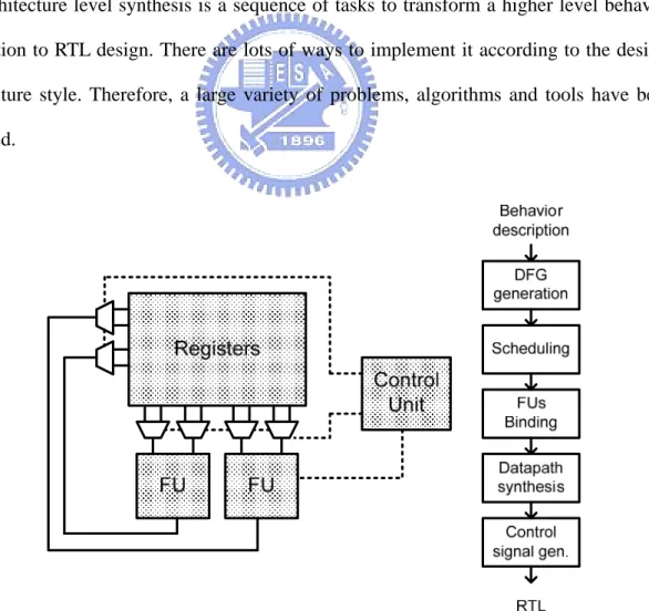
Fig. 1 shows a conventional and simplified architecture level synthesis system, which

includes target architecture and corresponding synthesis flow [14]. First, the synthesis

system will get the internal representation (i.e. data flow graph here) of design by compiling

input application. Second, the scheduling and binding tasks place operations in feasible

functional units and timing slots in sequencing order. Finally, it generates the detailed

interconnections and corresponding control signals which map the behavior of data transfer

and all configurations to circuit cycle by cycle.

This target architecture shown in Fig. 1 has some functional units, centralized register and

a corresponding control unit. The centralized registers store all temporal data and provide

all operands to functional units. In the view of data transfer, we can say that the scheduling

and binding are the tasks which assign when and to where the temporal data go. In addition,

the datapath synthesis task generates the needed multiplexers, de-multiplexers and wires of

interconnections.

In centralized register architecture, any data generated from some functional unit will be

available for other ones at the next cycle. In other words, it always takes no additional cycle

to transfer data between functional units. However, it should pay the extra cycle time for

this convenience interconnection scheme. Furthermore, the cycle time equal the

computation time plus interconnection delay which includes the delay of multiplexers,

de-multiplexers and wires.

Distributed Register Architecture

In Deep Submicron Meter (DSM) technology, the wiring delay is no longer trivial [1]. It

will dominate the overall system delay gradually with the scale evaluation of process

technology which is due to RC delay, coupling noises, inductance, etc [2][3]. Obviously, the

latency at that time.

In such a situation, it is important to take the interconnection delay into consideration.

Because the interconnection delay information is only available after physical layout, the

conventional architecture level synthesis flow cannot obtain the accurate cycle time. To

overcome this problem, lots of researchers had used the estimated interconnection delay for

a higher level design of abstraction [4][5][6][7][8][9].

In architecture level synthesis, the targeted architecture and corresponding synthesis

algorithm will affect the effectiveness of exploiting the interconnection delay. Therefore, the

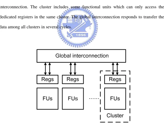
distributed register architecture which partitions the registers has been proposed [10][11].

Fig. 2 represents the simplified model, which has some clusters connected through global

interconnection. The cluster includes some functional units which can only access the

dedicated registers in the same cluster. The global interconnection responds to transfer the

data among all clusters in several cycles.

Additionally, some partition constraints prevent the overloading of interconnection delay

constituted by multiplexers (e.g. adding constraints on the number of access ports of

registers) and long wiring (e.g. adding constraints on the number of functional units).

Contrary to the conventional centralized register architecture, the distributed register

architecture partitions the interconnection delay in several cycles. Only the interconnection

delay within a cluster makes a portion in system cycle time. The other one in global

interconnection only makes the additional cycles. Therefore, the partition of interconnection

delay implies multi-cycle communication which enables the parallel execution of

computations and data transfers.

Base on the same concept, the Regular Distributed Register (RDR) architecture was

proposed [12], which offers high regularity and direct support of multi-cycle

communication. The RDR architecture divides the entire chip into an array of clusters.

Fig. 3 shows an example of RDR architecture with 2 3× cluster array. For the highly regular advantage of RDR architecture, the information of inter-cluster and intra-cluster

interconnection delay can be accurately recorded in lookup tables and pre-computed once

the parameter of RDR structure (e.g. size of cluster, clock period) are specified.

1.3. Extra Wire Loading in RDR-based Architecture

The corresponding synthesis flow for RDR is MCAS (Architectural Synthesis for

Multi-cycle Communication). At the front end, after generating the Control Data Flow

Graph (CDFG) of application, the MCAS performs resource allocation, functional unit

binding and scheduling-driven placement in order. These tasks place the functional units to

clusters and assign the operations in CDFG when and where to be executed. At the backend,

MCAS performs register and port binding followed by datapath and distributed controller

generation. The experimental results reported in [12] shows 44% and 37% improvement on

average in terms of the cycle time and final latency for data flow intensive examples. It also

shows 28% and 23% improvement on average in terms of the cycle time and final latency

for designs with control flow.

However, the RDR architecture may introduce extra global wiring overhead in the

presence of many simultaneous data transfers, when each one requires a dedicated global

connection. The significant wiring overhead would eventually limit the scaling of the

application in RDR architecture. To overcome this problem, [13] presents an architecture

level synthesis solution, which is called RDR-pipe, to support automatic interconnection

pipelining extended from RDR. The interconnection pipelining potentially improves the

wiring utilization by sharing the wires between each pair of clusters. Compared to RDR

architecture, 28% global wire-length reduction is reported [13] in RDR-pipe architecture.

A good way to reduce resource demand is sharing. The interconnection pipelining

improves the wiring overhead by sharing the wires between each two clusters. However,

this methodology still limits the sharing capability to divided localized regions, because the

transferred data are still scheduled and allocated within dedicated wires. Therefore, a global

1.4.

might greatly minimize the interconnection overhead. In this thesis, we propose the formal

formulation of channel and register allocation problem in architecture level synthesis, which

captures the behavior of the transfer data at each cycle in distributed register architecture.

Therefore, base on the formulation, it can be extended to minimize the required

interconnection resource easily.

Thesis Organization

The rest of the thesis is organized as follows: chapter 2 addresses the channel and register

allocation problem. Then it gives a motivational example which shows the difference

between pervious methods and the desired optimal solution. Chapter 3 presents the detailed

description of the proposed ILP formulation including problem formulation, variables

definition, constraints and the objective function. Chapter 4 gives some useful extensions to

the ILP model described in Chapter 3. Chapter 5 shows the experimental results compared

2.1.

Chapter 2 Channel and Register Allocation Problem

In this chapter, we introduce the channel and register allocation problem in architecture

level synthesis which has distributed registers. After that, a motivational example is given to

show why we need a new methodology to share the interconnection resource globally.

Channel and Register Allocation Problem

The RDR architecture gives lots of dedicated interconnection wires between clusters.

Because it has no interconnection pipelining, the sender will hold the transferred data for

several cycles. Therefore, one transferred datum will occupy a long wire for several cycles,

which wastes the interconnection resource.

The RDR-pipe is extended from RDR. It puts the registers in appropriate positions to

pipeline the long wires. By performing the transfer scheduling, it has higher utilization in

wiring resource. However, the register station in RDR-pipe has no control signal. It makes

the pipeline register dedicate to its interconnection wire only and cannot be shared for the

data generated from the other clusters.

Therefore, we address a further extension on the register station, which is capable of

incoming data and forward them to any directions. Besides, we take the distributed wiring

segments in available channels between register stations instead of the dedicated

interconnection. That is, any interconnection can be combined by several wiring segments.

Consequently, how to allocate those transfers to channels becomes a new problem because

the behavior of transfers deeply affects the interconnection resource including wires and

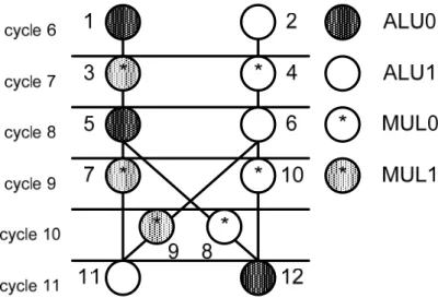
Fig. 4. Scheduled and bound DFG of DCT

The given input of this problem is the scheduled and bound data flow graph and

placement of functional units in distributed register architecture. The given input should be

checked whether the transfer latency is enough in advance. Fig. 4 shows a data flow graph

of discrete cosine transform [12] with two ALUs and two multipliers. Each circle which is

bound to a specific functional unit represents an operation. Also, these operations are

scheduled in a time slot divided by horizontal lines. The scheduled and bound data flow

graph describes when and which FU should take the temporary data to be computed.

Fig. 5 shows a cluster array architecture and the placement of two ALUs and two

multipliers. One cluster includes a meshed square as FUs which only access the dedicated

registers in the white square called register station. According to the placement of functional

units in

3 3×

Fig. 5(a) and the bound DFG, Fig. 5(b) replaces the relative operations in it.

Therefore, with the scheduling and binding information, we can specify the transfer where

Fig. 5. Placement functional units in distributed register architecture

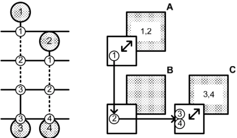
2.2. Previous Methodology

Because the channel and register allocation problem is extended from the

RDR/RDR-pipe architecture, we take those register and port binding tasks as the pervious

work. Fig. 6 shows a simple example of the scheme performed in RDR/MCAS. The

operation number 1 and 2 are executed in cluster A and the number 3 and 4 are in cluster C.

According to this architecture, the register 1 and 2 of sender A hold these transferred values

at least two cycles. Therefore, two parallel inter-cluster wires are needed between cluster A

and C for the overlap transfer time of data.

Fig. 7. Register and port binding task with dedicated pipelining interconnection

Fig. 7 performs the scheme of RDR-pipe/MCAS-pipe in the same example. With the

presence of pipeline register 2 in cluster B, register 1 can forward one data to register 2 at

the first cycle and forward the other one at the next cycle. These two data were issued at

different cycles and forwarded by pipeline register (i.e. register 2) without stalling until

reaching the cluster C. With transfer scheduling, it serializes the transfers by differing the

issued cycle of each datum. Therefore, only one interconnection wire is needed and it has

one wire reduction compared to RDR/MCAS.

2.3. Motivational Example

Sharing is the way to reduce resource requirement. We take a motivational example to

illustrate how the sharing capability affects the requirement of interconnection resource.

The comparison of results among RDR/MCAS, RDR-pipe/MCAS-pipe and the idealized

global sharing method will be discussed. Fig. 8 gives the scheduled and bound data flow

graph and the mapping of operations in a 3 3× cluster array. For comparing the result of resource requirement, we will count the number of registers and the wiring segments. A

simple definition of wiring segment is one wire between two adjacent clusters. The

Fig. 8. Given scheduled, bound DFG and placed functional units

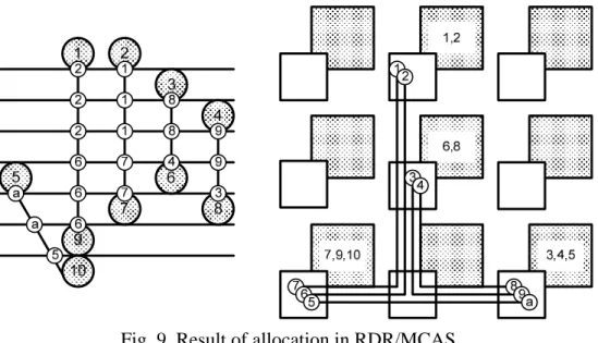
Fig. 9 shows the result of transfer allocation in RDR/MCAS. The cluster generating data

always holds the transferred value until the slack time equal to the interconnection delay.

No transfer scheduling and pipeline register makes extra wiring requirement. It needs 12

wiring segments and 10 registers in total.

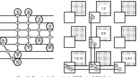
Fig. 10 shows the result of data transfer in RDR-pipe/MCAS-pipe. The pipeline registers

are inserted in each register stations where interconnections would pass away. Besides, the

transfer scheduling is performed to minimize the wire requirement. Consequently, it reduces

the wiring segments to 7 at the cost of additional 2 registers (i.e. totally 12 registers).

Fig. 10. Result of allocation in RDR-pipe/MCAS-pipe

The sharing of wires and registers by transferred data reduce the resource requirement.

Under the principle, we extend the capability of register stations which can store data for

cycles and forward them to arbitrary directions. The extension enables the transfer data use

all interconnection wires and registers. Therefore, it implies global sharing and more

resource reduction. Fig. 11 shows the result, with the hand-scheduling, it use only 4 wire

segments and 7 registers.

Chapter 3 Proposed ILP Formulation for the Channel

and Register Allocation Problem

In the chapter, we will formulate the behavior of transfers in distributed register

architecture with extended capability, which permits the register station to store or forward

data at each cycle. In our proposed formulation, the definition of problem and input will be

given initially. Then we will make an explanation of variables and decide the feasible region

of them. Finally, we will write down the objective function to minimize interconnection

resources which should be subject to uniqueness, continuity and resource counting

constraints.

3.1. Definition of Problem Given

Before solving the channel and register allocation problem, we assume the tasks of

scheduling and functional unit binding have been performed. Therefore, the scheduled and

bound data flow graph, functional unit placement are taken as input. Besides, the topology

information including the position and connectivity of clusters is also needed.

First, we use the graph representation to describe the input data flow graph.

The vertex set

( , ) S S S G V E { | 0,1, 2, ,| | 1} S i S V = o i= … V − k

represents the operations in data flow graph.

The directed edge set represents the data dependency

implying data transfer, such that means the data generated from { | 0,1, 2, ,| | 1} S i S E = e i= … E − : i j e o →o o_j should be sent to o_k.

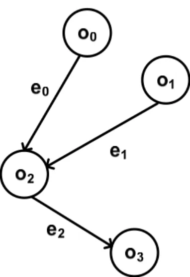
Fig. 12. Data flow graph as input application

Fig. 12 is a simple example of data flow graph, which has the vertex set

and the edge set { | 0,1, 2, 3} S i V = o i= E_S ={ |e i_i =0,1, 2} such that , and . 0: 0 e o →o₂ 2 3 1: 1 e o →o e₂:o₂ →o

Second, we use the graph representation , called topology information, to

specify the target distributed register architecture, which indicates the available positions for

putting interconnection wires or registers. The vertex set ( , ) T R W G V E { | 0,1, 2, ,| | 1} R i R V = r i= … V −

represents the register stations. The directed edge set E_W ={w i_i| =0,1, 2,…,|E_W | 1}− represents the available channels, such that we can describe the behavior of transferred data

from r_j to as . It is notable that we can use a self loop to enable the transferred data stay at the same register station for one cycle.

k

r w r_i: _j →r_k

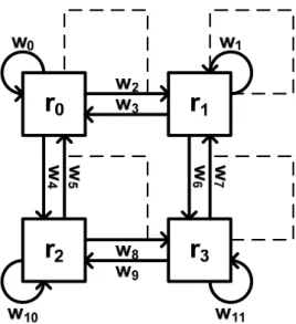
Fig. 13 takes a cluster array of distributed register architecture as topology

information, which has the vertex set 2 2×

{ | 0,1, 2,3}

R i

V = r i= and the edge set implying the register station has the capability to transfer data to

adjacent one horizontally, vertically by , or keeping them for cycles by

. { | 0,1, 2, ,11} W i E = w i= … 2, ,3 , 7 e e … e 0, , ,1 8 9 e e e e

Fig. 13. Topology information

The input data flow graph is scheduled and bound. What do the “scheduled” and “bound”

mean for? First, we can treat each data dependency in data flow graph as a transfer. Besides,

by the “scheduled” and “bound” information, we can know when these operations are done

and in which cluster the outputs are stored. In fact, we can use this information with

placement of functional units to specify each transfer like this statement – some transfer

is the task that taking data from register station

i

e

x

r to r_y from cycle to n m. Precisely, we can use a set of pair {et_i =(st ft_i, _i) |e_i∈E_S} to specify the transfer generated at cycle and required at cycle

i

e

i

st ft . And another set of pair is used to specify _i

the transfer e_i generated at register station sr_i and required at register station fr . _i

In Fig. 14, we focus on the edge , which is a data dependency between and .

By the information of and , we could know there is a datum needed to be

transferred from register station

0

e o₀ o₂

0

et er₀

0 1

sr = at cycle st₀ = to register station 5 fr₀ = at 2 cycle ft₀ =8.

Fig. 14. Specification of a transfer

3.2. The Definition of Variables

How to define appropriate variables is important, which affects the complexity, flexibility

of an ILP formulation. To minimize the limitation of extension capability in our proposed

formulation, we decide to capture the basic behavior of transfer at each cycle. Without lots

of indirect specifications, a simple type of zero-one integer variable x_{i j k, ,} is adopted and called channel allocation variable.

w2 w3 w8 w9 r3 w0 w1 w10 w11 o0 o1 o3 e0 cycle 6 cycle 7 cycle 8 cycle 9 cycle 5 et0= (5 , 8) er0= (1 , 2) r1 r2 r0 o2

The meaning of x_{i j k, ,} is that whether the transfer datum e_i at cycle j is allocated to

channel w_k. “One” value means yes, and “zero” stands for no. The set X collects all these zero-one variables and can be written as:

, ,

{ _{i j k} | 0,1, ,| _S | 1; _{i i}; 0,1, | _W | 1}

X = x i= … E − ft ≥ >j st k= … E −

How do these variables work for describing a transfer path? Fig. 15 shows an example.

In this example, transfer should be taken from register station to from cycle 6 to

8. If we have chosen a transfer path, which is sending the data to at first cycle, staying

one cycle in at next step and achieving in the end of cycle 8. What we need to do is

specifying this path by setting variables

0 e r₁ r₂ 0 r 0 r r₂ 0,6,3

x , x_0,7,0 and x_0,8,4, which means using the

channels , and respectively cycle by cycle. Then preserve the other allocation

variables of transfer to zero for preventing the ambiguity in assignment of transfer

behavior. Therefore, one assignment of allocation variables without ambiguity stands for

one transfer behavior of data. It is the one to one and onto mapping implying that the entire

solution space is included in the variety of assignment.

3

w w₀ w₄

0

e

Otherwise, to minimize the interconnection resource, the counting resource variables are

also defined. The interconnection resource includes wires and registers. In our formulation,

we care about the resource requirement in available channels and register stations.

Therefore, the straightforward types of integer variables, and , are used. They

mean the number of wires in available channel and registers in available register

station , respectively. i Nw Nr_i i w i r

3.3. The Feasible Region of Variables

In fact, there are lots of redundant allocation variables included in the set X . With the

specification of generating and requiring register stations, the active region of transferred

data is limited. That is, there are lots of channels of transfers would never be used, and these

corresponding allocation variables are always zero. To minimize the allocation variables

while preserving complete behavior of transfer, it is needed to decide the feasible activitive

region of transfer at each cycle.

As mention above, the activity region of transfer is limited by generating and requiring

register station. We take the same example in Fig. 16. Fig. 16(a) shows that the possible

channels used for transfer at cycle 6. Those feasible channels are limited to ,

and , which are all emitted from generating register station . Even at the next cycle,

the feasible channels are also limited to those ones emitted from register stations ,

and . Therefore, the feasible channels are spread out from generating register station and

the effect of limitation can be traced cycle by cycle. Base on this idea, we define the set

which includes the number of feasible channels traced from the generating register

station at cycle j: 0 e w₁ w₃ 6 w r₁ 0 r r₁ 3 r , i j WS i sr , 1 , ( ) , 1 { | : , } , 1 i j i i i k WS i j k sr m k W i NW k ft j st WS k w r r w E j st − ∈ ⎧ ≥ > + ⎪ = ⎨ → ∈ = + ⎪⎩

∪

Such that ( ) { | _i: _{x y}, :_{j y z}; ,_{i j W}} NW i = j w r →r w r →r w w ∈E

Fig. 16. Limitation of activitive region of transfer

The WS_{i j,} is defined recursively and takes the generating cycle as the initial condition. Fig. 17 shows an example. The set of feasible channels of transfer e₀, which is equal to WS_0j, has carried out. The includes channel 1, 3 and 6 which are all leaving from the

generating register stations and entering into , , or . At the next cycle, the

should include those channels leaving from , , or . We can get in the same

manner. 0,6 WS 1 r r₀ r₁ r₃ WS_0,7 0 r r₁ r₃ WS_0,8

On the other side, Fig. 16(b) shows that the possible channels used for transfer at

cycle 8. Those feasible channels are limited to , and , which are all achieving

requiring register station . Therefore, the feasible channels at the last cycle, or cycle 7,

are limited to those entering into register stations , or . Base on the same idea,

these traceable feasible channels spread out from requiring register station

0 e 4 w w₉ w₁₀ 2 r 0 r r₂ r₃ i fr of transfer

at cycle j can be collected in the other sets :

i e WF_{i j,} , 1 ( ) , 1 { | : , } , i j i i i k WS ij k m fr k W i LW k ft j st WF k w r r w E j ft + ∈ ⎧ > ≥ + ⎪ = ⎨ → ∈ = ⎪⎩

∪

Such that ( ) { | _j: _{x y}, :_{i y z}; ,_{i j W}} LW i = j w r →r w r →r w w ∈E

Fig. 17. Tracing feasible channels from generating register station

The WF_{i j,} is defined recursively and takes the requiring cycle as the initial condition. Fig. 18 shows the same example in Fig. 17 and contrarily traces from the other side. The

includes channels 4, 9 and 11 which are all achieving the requiring register stations

and are leaving from , or . At the last cycle, or cycle 7, the should

include those channels entering into , or . Then we can get in the same

manner. 0,8 WF 2 r r₀ r₂ r₃ WF_0,7 0 r r₂ r₃ WF_0,6

The set and collect the feasible channels from contrary side of register

stations of transfers. Therefore, the new set generated by intersecting and

can delete all the redundant candidates and preserve the capability of representing all

possible transfer paths at the same time. It can be written as:

, i j WS WF_{i j,} , i j W WS_{i j,} , i j WF , , , i j i j i j W =WS

∩

WF , i j

W describes the activity region of transfer, which are the all possible number of

feasible channels of transfer e_i at cycle j. By this information, the set X_{i j,} including all feasible channel allocation variables of transfer at cycle j could be easily written as

follow: i e , { , , | , i j i j k i j X = x k∈W }

Table 1 follows the example in Fig. 17 and Fig. 18, and generates W_0,j set by intersecting WS_0,j and WF_0,j. Therefore, we can find the feasible channel variables of transfer e0 at cycle 6, cycle 7 and cycle 8 are as followed, respectively:

0,6 0,6,1 0,6,3 0,6,6 0,7 0,6,0 0,6,3 0,6,4 0,6,6 0,6,9 0,6,11 0,8 0,6,4 0,6,9 0,6,10 { , , }; { , , , , , } { , , }; X x x x X x x x x x x X x x x = = = ;

Tab. 1. Possible channels of transfer e₀ in Fig. 17 and Fig. 18

J (cycle) WS0,j WF0,j W0,j

6 {1,3,6} (0~11) {1,3,6} 7 {0,1,2,3,4,6,7,9,11} {0,3,4,5,6,8,9,10,11} {0,3,4,6,9,11} 8 {0~11} {4,9,10} {4,9,10}

Addition to allocation variables, we also give the upper bound of resource counting

variables. It is useful for the requirement evaluation of interconnection resource and being

an effective limitation of the variable range in generic ILP solver. The idea is that the

numbers of interconnection resource, which are wires in channels or registers in register

stations, are not more than the possible maximum requirement of all cycles. To do this, we

define the set Rw_{k j,} including all the numbers of transfer. It is possible for all the numbers of transfer to be allocated in channel w_k at cycle j:

, { | , , }

k j i j k

Rw = i x ∈X

With the same idea, Rr_{k j,} is defined to include all the numbers of transfer. It is possible for all the numbers of transfer to be allocated and entered into register stationr_k at cycle j:

, { | : , },

y j k x y R i j k,

Rr = i w r → ∈r E x ∈X

Finally, find the maximum in these sets, which will be the upper bound of the

corresponding resource requirements. The upper bound of the number of wire segments in

channel w_k could be written as:

,

upper bound of Nw_k =max({|Rw_{k j}|| j=0,1,…,|T| 1})−

The upper bound of number of registers in register station r_k could be written as:

,

upper bound of Nr_y =max({|Rr_{y j}|| j=0,1,…,|T| 1})−

3.4. The Objective Functions and Subjected Constraints

With the previous definition, we can write down our objective function, which is the

summation of all weighted required resources:

| | 1 | | 1 0 0 W R E V i i i i i i Nr Nw α β − − = = +

∑

∑

It is notable that the constant factors α_i and β_i weight the affection of resource types, and usually the weight of self loop which implies to stay one cycle is set to zero. However,

there are some constraints which the formulation should be subject to will preserve the

correctness of transfer behaviors.

The first are the Uniqueness constraints, which describe that the channel allocation of

each transfer should be unique at each cycle. More than one channel allocated at the same

cycle will make ambiguity. The uniqueness constraints can be written as:

, , , =1, | | 0, i j i j k s i i k W x E i ft j s ∈ > ≥ ≥ >

∑

t

It makes a summation of all objects in each set X_{i j,} and forces it to one. These constraints imply that only one allocation variable could be set at one cycle and prevent the

ambiguity of transfer behavior. Fig. 19 shows an example that transfer should be

assigned a transfer path from register station 1 to 2 from cycle 6 to 8. Then the allocation

should subject to the uniqueness constraint written as:

0 e 0 , 0, , =1, 8 5; j j k k W x j ∈ ≥ >

∑

The expanded equations are followed for cycle 6, cycle 7 and cycle 8, respectively:

0,6,1 0,6,3 0,6,6 0,7,0 0,7,3 0,7,4 0,7,6 0,7,9 0,7,11 0,8,4 0,8,9 0,8,10 1, 1, 1; x x x x x x x x x x x x + + = + + + + + = + + =

The second one are the continuity constraints, which describe that the transfer at two

consecutive cycles must be continuous in feasible channels. These constraints hold the

transfer path available, that is, the register station allocated channel entering into must be

the same one allocated channel leaving from at next cycle. The continuity constraints can be

written as: , 1 , , , 1, ( ) 0, | | 0, , | | 0; i j i j k i j k s i i W k NW k W x x E i ft j st E + ′ + ′∈ − +

∑

≥ > ≥ ≥ > > ≥k ∩

o0 o2 o1 o3 e0 cycle 6 cycle 7 cycle 8 cycle 9 cycle 5 W0,j J (cycle) 6 7 8 {0,3,4,6,9, 11} {1,3,6} {4,9,10} w2 w 7 w 5 w 4 w8 w9 r0 r2 r3 w0 w10 w11 w3 w 6 r1 w1 et0= (5 , 8) er0= (1 , 2)

Fig. 19. Uniqueness constraints of transfer e₀ at cycle 6

It describes that if the allocation variable entering into register r at cycle j is set, then _x

one of those variables which is leaving from r must be set at cycle _x to hold the continuity of the transfer path. Any channel allocation variable has its own continuity

constraints, except for those ones at the last transfer cycle. Because only the chosen

allocation variable should hold this constraint, the inequality (i.e. relation of larger than)

exists to prevent the violation from the other unset ones. With the same example shown in 1

j+

Fig. 19, the constraints could be expanded as follows:

At cycle 6, 0,6,1 0,7,3 0,7,6 0,6,3 0,7,0 0,7,4 0,6,6 0,7,9 0,7,11 0, 0, 0; x x x x x x x x x − + + ≥ − + + ≥ − + + ≥ At cycle 7, 0,7,0 0,8,4 0,7,3 0,8,4 0,7,4 0,8,10 0,7,6 0,8,9 0,7,9 0,8,10 0,7,11 0,8,9 0, 0, 0, 0, 0, 0; x x x x x x x x x x x x − + ≥ − + ≥ − + ≥ − + ≥ − + ≥ − + ≥

Additional to hold the correctness of transfer behavior, the other constraints make the

number of interconnection resource enough to transfer all the data. The number of wires in

channel is represented by the wiring counting variable , and the number of

registers in register station is represented by register counting variable . However,

they must be more than the amount of the requirement at each cycle. For the wire counting

variable, this can be addressed as:

i w Nw_i i r Nr_i ≥ > ≥ , , , , , 0, | | 0, | | 0 i j k i j k i j k W x X Nw x E k T j ∈ −

∑

≥ > ≥ >

Each wiring counting variable has a set of constrains which are formulated to check

whether the number of wires is sufficient. The number of constraints in a set we need to

written down is equal to the total cycle counts. And with the same idea, the constraints of

register counting variables are:

, , , , , { | : , } { | } 0, | | 0 k x y k W i j k i j y i j k k w r r w E i x X Nr x T j → ∈ ∈ −

∑

∑

≥

Likewise, each register counting variable has a set of constrains which are formulated to

check whether the value of counting variable is sufficient. The number of constraints in a

set we need to write down is equal to the total cycle counts. The example is shown in Fig.

20, which specifies another transfer . The constraints checking the resource variables are

written as follows:

1

e

For wire counting variable 0 0,7,0 1 0,6,1 3 0,6,3 3 0,7,3 4 0,7,4 4 0,8,4 6 0,6,6 6 0,7,6 0, 0, 0, 0, 0, 0, 0, 0, Nw x Nw x Nw x Nw x Nw x Nw x Nw x Nw x − ≥ − ≥ − ≥ − ≥ − ≥ − ≥ − ≥ − ≥ 9 0,7,9 1,7,9 9 0,8,9 1,8,9 10 0,8,10 1,8,10 11 0,7,11 1,7,11 0, 0, 0, 0, Nw x x Nw x x Nw x x Nw x x − − ≥ − − ≥ − − ≥ − − ≥

For register counting variable

0 0,6,3 0 0,7,0 0,7,3 1 0,6,1 2 0,7,4 0,7,9 1,7,9 2 0,8,4 0,8,9 0,8,10 1,8,9 1,8,10 3 0,6,6 3 0,7,6 0,7,11 1,7,11 0, 0, 0, 0, 0, 0, 0, Nr x Nr x x Nr x Nr x x x Nr x x x x x Nr x Nr x x x − ≥ − − ≥ − ≥ − − − ≥ − − − − − ≥ − ≥ − − − ≥

Chapter 4 Useful Extension on the ILP Formulation

With the high flexibility, the extensions of model, objective function, or specific behavior

of transfer could be introduced in our proposed ILP formulation. Therefore, in this chapter,

we will give two useful extensions. One is the further reduction on requirement of

interconnection resource, which is called resource counting problem. The other one is

modeling the transfer behavior of the bi-directed channel from existing directed ones.

4.1. Resource Counting Problem

In some case, the resource requirement would be overestimated. That is, when more than

one data outputted from the same operation and allocated in the same channel, they would

be counted owning individual one channel requirement and result in two wire requirements.

In other words, the formulation would use more wires to transfer the same datum. Thus, the

resource requirement has been overestimated. Not only the wire segments in channel, but

also the registers in register station would face this problem. Fig. 21 shows the example

which experiments this situation. In this example, transfer and outputted from

operation are assumed to be the same datum. From the previous resource constraints

written as: 3 e e₄ 3 o 2 3,11,2 4,11,2 4 4,11,4 6 4,12,6 8 4,12,8 1 3,11,2 4,11,2 2 4,11,4 3 4,12,6 4,12,8 0, 0, 0, 0, 0, 0, 0, Nw x x Nw x Nw x Nw x Nr x x Nr x Nr x x − − ≥ − ≥ − ≥ − ≥ − − ≥ − ≥ − − ≥

Fig. 21. Resource counting problem

There are at least two wires in channel and two registers in register station

counted for the final adoption of path by transfer . However, they are all

overestimated by one.

2

w r₁

2 6

(w w, ) e₄

To overcome this problem, new zero-one integer variable are introduced instead

of original , , m j k c , , i j k

x . The meaning of is that, whether there is any datum from the

operation allocated to the channel at the cycle j. It implies not only capturing the

behavior of each transfer datum, but also checking which operation they come from.

, ,

m j k

c

m

o w_k

To find out the fixed allocation variables , we use the new set to collect

those original allocation variables

, ,

m j k

c Ym j k, , , ,

i j k

x generated from operation and allocated in

channel at cycle

m

o

k

e j . The definition could be written as:

, , { , , | , , , ; (e : )

m j k i j k i j k i j x m S

Y = x x ∈X o → ∈E }

Therefore, we can get the fixed allocation variables c_{m j k, ,} from original ones x_{i j k, ,} and the set Y_{m j k, ,} by the equation:

, , , , , , , , , , , , { | } | | | | i j k m j k m j k m j k m j k i j k i x Y Y Y c x ∈ > −

∑

≥0

then the variables will be set to one. On the other hand, the variables will be

forced to zero if the summation is equal to zero. These variables represent the exactly

requirement of wires by resource sharing of the same datum. Four new sets , ,

and which is the transferred data outputted from have been generated:

, , m j k c c_{m j k, ,} 3,11,2 Y Y3,11,4 3,12,6 Y Y3,12,8 o3 } , 3,11,2 3,11,2 4,11,2 3,11,4 3,11,4 3,12,6 3,12,6 3,12,8 3,12,8 Y ={x , x Y ={x } Y ={x } Y ={x }

we now deduced the corresponding fixed channel allocation variables , ,

and by: 3,11,2 c c_3,11,4 3,12,6 c c_3,12,8 3,11,2 3,11,2 4,11,2 3,11,4 3,11,4 3,12,6 3,12,6 3,12,8 3,12,8 2 2 ( ) 0 1 0, 1 0, 1 0; c x x c x c x c x > − + ≥ > − ≥ > − ≥ > − ≥

Two things are worth to observe. First one is that, if the Y_{m j k, ,} includes only one object

, ,

i j k

x , than we can get the result c_{m j k, ,} =x_{i j k, ,} , which implies the conversion process affects nothing. The allocation variables , and are in this situation. The second

one is shown in the fixed allocation variable . The corresponding set has more

than one object, which are and . The is always taken for the correctness

of transfer . Therefore, No matter the is adopted by transfer or not, the

is always one. That is, the fixed variable marks only whether the data outputted from

at cycle 3,11,4 c c_3,12,6 c_3,12,8 3,11,2 c Y_3,11,2 3,11,2 x x_4,11,2 x_4,11,2 4 e x_3,11,2 e3 c3,11,2 , , m j k c m

Finally, we use these new fixed channel allocation variables instead of original ones to

count the interconnection resource. The resource counting constraints are rewritten as

follows: > ≥ > ≥ , , , , , , , , { | } , , { |( : ) } { | } 0, | | 0, | | 0 0, | | 0 m j k m j k y W m j k m j k m j k W m c Y y i j k k w r E m c Y Nw c E k T j Nr c T j ∈ → ∈ ∈ − ≥ > ≥ − ≥

∑

∑

∑

The new constraints take the c_{m j k, ,} and Y_{m j,} instead of x_{i j k, ,} and X_{i j,} and these constraints of example in Fig. 21 for cycle 11 to 12 are also shown here:

2 3,11,2 4 3,11,4 6 3,12,6 8 3,12,8 1 3,11,2 2 3,11,4 3 3,12,6 3,12,8 0, 0, 0, 0, 0, 0, 0, Nw c Nw c Nw c Nw c Nr c Nr c Nr c c − ≥ − ≥ − ≥ − ≥ − ≥ − ≥ − − ≥

4.2. Integrating Bi-directional Channels in the Model

To minimize the wiring overhead, the bi-directional channel is usually considered in the

scope of design methodology. There are two ways to achieve the goal in our proposed ILP

formulation. One is introducing the new bi-directional wires in topology information and

making some modification in continuity constraints, resource counting constraints and

Fig. 22. Modeling the bi-directional channel

We take a new example in Fig. 22. It should transfer one datum from to , and

the other two data and from to at cycle 15. The new bi-directional channel

5

e r₀ r₁

6

e e₇ r₁ r₀

12

x is used to share the transfer loading instead of only directed ones (i.e. and ).

Intuitively, at cycle 15 we can write down the substitute resource counting constraints as

follows: 2 w w₃ 2 5,15,2 3 6,15,3 7,15,3 12 5,15,12 6,15,12 7,15,12 0 ( ) 0 ( ) Nw x Nw x x NB x x x − ≥ − + ≥ − + + ≥0

This method is straightforward, but it introduces lots of additional allocation variables. In

the worst case, if we take bi-directional channels beside all directed pairs of wires which are

mutually inverse, they will introduce at most two times of original allocation variables in

our ILP formulation. These additional variables will be a nightmare for the ILP solver

especially in a great scale application.

The other way to reach the goal is using post processing. In fact, the original formulation

with only directed channels has captured enough information about the behavior of transfer.

All we need to do is to decide who should take these transfers loading, the directed channel

or bi-directional one? In other words, the original directed channels could be treaded as the

the feasible channel allocation by these permissions, we choose the type of interconnection

resources to take these possible loadings. It has the modification in resource counting

constraints, which adds the new term SB . This new term is the transfer resource supported _x

by additional bi-directional channels:

, , , , , { | } 0, | | 0, | | 0 i j x i j x x i j x W i x X Nw SB x E x T j ∈ + −

∑

≥ > ≥ > ≥

The third term is the transfer requirements, the first and second ones could be treaded as

two types of transfer resource sharing the loading together. Because of the bi-direction of

channel, there is another side of transfer written as:

, , , , , { | } 0, | | 0, | | 0 i j y i j y y i j y W i x X Nw SB x E y T j ∈ + −

∑

≥ > ≥ > ≥

Thus, the added bi-directional channels represented by the resource counting variable

,

x y

NB take the loading from w and x at the same time. Hence, it should subject to the

resource counting constraints which could be written as:

y

w

, 0, | | 0

x y x y

NB −SB −SB ≥ T > ≥j

The same example in Fig. 22 could be reformulated with this post processing:

2 2 5,15,2 3 3 6,15,3 7,15,3 2,3 2 3 0 ( ) 0 Nw SB x Nw SB x x SB SB SB + − ≥ + − + ≥ − − ≥ 0

Finally, the rest work would give the weight of resource overhead on directed channels

(i.e. , ) and bi-directional channel (i.e. ) individually in the objective

function. In summary, this type of formulation takes only some post processing without

introducing any additional allocation variables.

2

5.1.

Chapter 5 Experimental Result

In this chapter, we will introduce the pre-work of our experiment initially. Then the

experimental results compared to the two previous works will be presented. Finally, we will

give a brief summary about this experiment.

Pre-work for the Input of Experiment

One of the input source in the channel and register allocation problem is the scheduled

and bound data flow graph and the placement of functional units. For getting this

information, we construct a simplified architecture level synthesis flow including these

tasks - data flow graph generation, scheduling, functional units binding and placement of

functional units with rescheduling. However, the synthesis flow does not address any

performance issue (e.g. cycle time or overall latency). It is just generating the inputs of our

experiments.

This synthesis flow takes the c++ code as input application. First, the task of data flow

graph generation takes the SUIF compiler infrastructure [17] as the front end and generates

the virtual machine codes by Machine SUIF [18]. Then we convert the internal

representation of this code to our desired data flow graph. Second, we use force-directed

scheduling with the minimal cycle timing constraints [15] to get the resource allocation and

the initial scheduled data flow graph. Third, an approximate max-clique based algorithm

[14] is performed to assign the operations in data flow graph to functional units. Fourth, we

randomly put the functional units to cluster and perform rescheduling, because of adding

multi-cycle interconnection. Finally, we have got the final scheduled and bound data flow

Fig. 23. The target architecture in experiment

The other input of our experiment is the topology information which has the specification

of distributed register architecture. In out experiment, we use a 3 3× cluster array with vertical and horizontal adjacent connectivity as our target architecture. There are 9 available

register stations and 33 available directed channels including 9 self loops shown in Fig. 23.

The system is implemented in C++/UNIX environment and using the lpsolve version

5.5.0.0 [19] as the ILP solver.

5.2. Experimental Result

We take the source code of mpeg2enc, jpeg and rasta from Mediabench [16] as our input

applications and classify these operations into two functional unit types - ALU and

multiplier. One stage ALU and two-stage multiplier are adopted as our functional units.

We have implemented three methods including two previous works and the proposed ILP

formulation. For addressing the minimization on interconnection wires, we give the weight

ratio to register and wires are 5 to 1, that is

7 31 0 0

1

5

_j i j

Nr

_ι

Nw

= =

×

+

×

∑

∑

Tab. 2. Information of data flow graph in applications Resource (FU)# Node# ALU# MUL# Cycle Count (1) mpeg2enc (dfg 1) 66 5 2 23 (2) mpeg2enc (dfg 2) 101 9 4 23 (3) mpeg2enc (dfg 3) 196 18 8 18 (4) jpeg (dfg 1) 93 9 2 35 (5) jpeg (dfg 2) 109 9 2 33 (6) jpeg (dfg 3) 140 11 6 23 (7) rasta 119 7 5 33

Tab. 2 shows the information of each data flow graph in applications. The nodes in data

flow graph represent the operations. After initial scheduling, we can get the number of

ALUs and multipliers. Because of the functional placement, the final cycle count presents

after the rescheduling.

We implement three methods to solve the channel and register allocation problem.

Method 1 is the previous one which has dedicated interconnection wireS without pipelining.

Method 2 is also the previous work which pipelines the interconnection wires and performs

the transfer scheduling to improve the wiring overhead. The third method is our proposed

ILP model, which share all interconnection resource globally and solved by ILP solver.

The interconnection overhead including wires and registers are all the metrics to evaluate

the performance. Those results are shown in Tab. 3, which report the requirement of

Tab. 3. Experimental result in three methods

Method 1 Method 2 Method ILP

Ch# Reg# Ch# Reg# Ch# Reg# Run time (sec) (1) mpeg2enc (dfg 1) 42 28 37 45 25 25 0.16 (2) mpeg2enc (dfg 2) 76 53 60 76 42 38 102.58 (3) mpeg2enc (dfg 3) 130 92 109 133 68 61 6.26 (4) jpeg (dfg 1) 81 50 64 78 24 28 8.9 (5) jpeg (dfg 2) 78 44 59 68 28 28 0.98 (6) jpeg (dfg 3) 75 72 58 87 24 48 235.53 (7) rasta 74 56 57 75 25 27 340.11 average 79.43 56.43 63.43 80.29 33.71 36.43 normalized to Method 1 1 1 0.798 1.423 0.424 0.646

Method 1 uses lots of interconnection wires, which seems a nightmare for whole system.

Method 2 pipelines the interconnection wires and tries to share the dedicated wires between

each two clusters. It improves about 20% in wiring overhead but pays the 40% additional

registers cost. However, the sharing scheme of method 2 is limited to divided local region.

In our formulation, we try to let all transferred data share whole interconnection resource

by taking the wire segments instead of the dedicated interconnections. Besides, we also take

the pipeline registers as general ones. We enable a global sharing and using ILP solver to

find the optimal solution, which make around 60% and almost 45% improvement on

Chapter 6 Conclusions and Future Works

Base on the regular distributed register architecture, we extend the capability of register

stations and try to use the global sharing of interconnection resource to improve the wiring

overhead. We propose the channel and register allocation problem and give it a formal

formulation. This formal model has high flexibility to make lots of extension, because it

captures the basic behavior of transferred data at each cycle. Through ILP solver, we get the

optimal solution under some experimental specification. It results in 53% wires and 35%

registers improvement on average compared to previous methods. However, it must be

noticed that the ILP solver cannot deal with large scale applications. Thus, we still need to

Chapter 7 Reference

[1] International Technology Roadmap for Semiconductor. Semiconductor Industry

Association, 1999.

[2] D. Sylvester and K. Keutzer, “Getting to the bottom of deep submicron,” in Proc. Int’l

Conf. on Computer Aided Design, pp. 203–211, Nov. 1998.

[3] Y. I. Ismail, E. G. Friedman, and J. L. Neves, “Figures of merit to characterize the

importance of on-chip inductance,” IEEE Transactions on Very Large Scale Integration

(VLSI) Systems, vol. 7, Dec. 1999.

[4] S. Tarafdar, M. Leeser, and Z. Yin, “Integrating floorplanning in data-transfer based

high-level synthesis,” in Proc. Int’l Conf. on Computer Aided Design, pp. 412–417, Nov.

1998.

[5] J. P. Weng and A. C. Parker, “3D scheduling: high-level synthesis with floorplanning,”

in Proc. Design Automation. Conf., pp. 668–673, 1991.

[6] Y. M. Fang and D. F. Wong, “Simultaneous functional-unit binding and floorplanning,”

in Proc. Int’l Conf. on Computer Aided Design, pp. 317–321, 1994.

[7] P. Prabhakaran and P. Banerjee, “Parallel algorithm for simultaneous scheduling,

binding and floorplanning in high-level synthesis,” in Proc. Int’l Symposium on Circuits

and Systems, vol. 6, pp. 372–376, 1998.

[8] V. G. Moshnyaga and K. Tamaru, “A placement driven methodology for high-level

synthesis of sub-micron ASIC’s,” in Proc. Int’l Symposium on Circuits and Systems, vol.

[9] Y. Mori, V. G. Moshnyaga, H. Onodera, and K. Tamaru, “A performance-driven

macro-block placer for architectural evaluation of ASIC designs,” in Proc. The Eighth

Annual IEEE International ASIC Conference and Exhibit, pp. 233–236, 1995.

[10] J. Jeon, D. Kim, D. Shin, and K. Choi, “High-level synthesis undermulti-cycle

interconnect delay,” in Proc. Asia South Pacific Design Automation Conf., Jan. 2001, pp.

662–667.

[11] D. Kim, J. Jung, S. Lee, J. Jeon and K. Choi, “Behavior-to-Placed RTL Synthesis with

Performance-Driven Placement,” in Proc. Int’l Conference on Computer Aided Design,

pp. 320-326, 2001.

[12] J. Cong, Y. Fan, X. Yang and Z. Zhang, “Architecture and Synthesis for Multi-Cycle

Communication,” in Proc. 2003 International Symposium on Physical Design, pp.

190-196, Apr. 2003.

[13] J.Cong et al., “Architecture-Level Synthesis for Automatic Interconnect

Pipelining,” in Proc. DAC 04, June 2004, San Diego CA.

[14] G. D. Micheli, Synthesis and Optimization of Digital Circuits. McGraw-Hill, Inc., 1994.

[15] P. Paulin and J. Knight, “Force-directed scheduling for behavioral synthesis of ASICs,”

IEEE Trans. Computer-Aided Design, vol. 8, pp. 661–679, Jun. 1989.

[16] C. Lee, M. Potkonjak, andW. H. Mangione-Smith, “Mediabench: A tool for evaluating

and synthesizing multimedia and communications systems,” in Proc. Int. Symp.

Microarchitect., Nov. 1997, pp. 330–335.

[17] SUIF Compiler [Online]. Available: http://suif.stanford.edu.

[18] M. D. Smith and G. Holloway, “An introduction to machine SUIF and its portable

libraries for analysis and optimization,” in Division of Engineering and Applied