THE POSITIVE REAL CONTROL PROBLEM AND THE
GENERALIZED ALGEBRAIC RICCATI EQUATION FOR
DESCRIPTOR SYSTEMS
He-Sheng Wang
Center for Aviation and Space Technology Industrial Technology Research Institute
Hsinchu, Taiwan 310, R.O.C.
Chee-Fai Yung*
Department of Electrical Engineering National Taiwan Ocean University
Keelung, Taiwan 202, R.O.C.
Fan-Ren Chang
Department of Electrical Engineering National Taiwan University Taipei, Taiwan 106, R.O.C.
Key Words: positive real control, descriptor system, generalized
algebraic Riccati equation.
ABSTRACT
In this paper, some useful properties of generalized algebraic Riccati equations and generalized positive real lemma for descriptor systems are given. Based on these results, the main purpose of this paper is to investigate the positive real (PR) control problem for de-scriptor systems. Necessary and sufficient conditions are derived for the solution to this problem expressed in terms of two generalized al-gebraic Riccati equations which may be considered to be generaliza-tions of the Riccati equageneraliza-tions obtained by Sun et al. (1994). When these conditions hold, state space formulae for all controllers solving the problem are also given.
*Correspondence addressee
I. INTRODUCTION
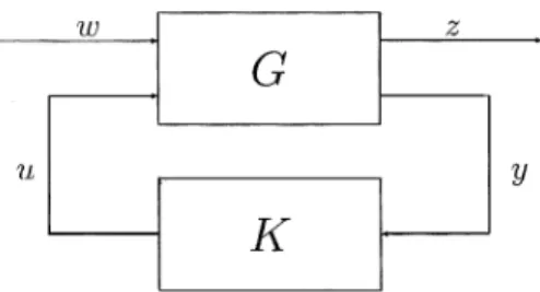
Consider the standard block diagram shown in Fig. 1. In our problem, the plant G is a descriptor system described by the following dynamical equations:
Ex =Ax+B1w+B2u,
G=GOF=∆ z =C1x+D11w+D12u, Ex(0–)=Ex0 given,
y =C2x+D21w, (1)
(the subscript “OF” stands for output feedback) where x∈IRn is the state, and w∈IRp represents a set of ex-ogenous inputs which includes disturbances to be re-jected and/or reference commands to be tracked. z∈IRp is the output to be controlled and y∈IRl is the measured output. u∈IRm is the control input. A, B
1, B2, C1, C2, D11, D12, and D21 are constant matrices with compatible dimensions. E∈IRn×n and rankE=r <n.
system described by K = KOF= ∆ E0x0= A0x0+ B0y , u = C0x0 (2)
where x0 is the state of the controller. Note that the plant and the controller are assumed the same struc-ture but they may have different E matrices. The ob-jective of the control is to internally stabilize G such that the closed-loop transfer function Tzw is extended
strictly positive real (ESPR, see section III for a pre-cise definition). Here closed-loop internal stability means that the closed-loop system is regular, impulse-free, and that the states of G and K go to zero from all initial values when w=0.
This problem, referred to as the ESPR output feedback control problem, has been recently ad-dressed and extensively studied in Sun et al. (1994) for linear time-invariant (LTI) plant and controller in state space model, in which several necessary and sufficient conditions in terms of solutions to algebraic Riccati equations or inequalities(ARE or ARI) were proposed for the solvability of the ESPR control problem. State-Space formulas for the controller de-sign were also given in Sun et al. (1994). Most recently, Yung (1999) has characterized all solutions to this problem. He also adopted state space formulation.
The most general motivation for studying this problem stems from robust and nonlinear control: If the system uncertainties (linear and/or nonlinear) can be characterized by positive real properties, then the classical results in stability theory can be used to guarantee robust stability provided an appropriate closed-loop system is strictly positive real(Popov, 1973; Zames, 1966a, 1966b). Other materials come from circuit theory (Anderson, 1973) adaptive con-trol (Astrom, 1983) and stability analysis (Narendra, 1973; Popov,1973). It is beyond the scope of this paper to review the vast literature associated with positive realness theory. For a more extensive bibli-ography and review of the literature, see, e.g., Ander-son et al. (1973), Joshi (1989), Narendra et al. (1973), Safonov et al. (1987), Sun et al. (1994), and the ref-erences cited therein.
The main point of this paper is that we adopt the descriptor systems model rather than the state space model. The control theory based on descriptor system models has been widely developed for many years: Cobb (1983) first gave a necessary and suffi-cient condition for the existence of an optimal solu-tion to the linear quadratic optimizasolu-tion problem and also extensively studied the notions of controllability, observability and duality in descriptor systems (Cobb, 1984). The notions concerning controllability and observability for descriptor systems will not be reproduced here. See, e.g., Armentano (1986), Cobb (1984) for details. The generalized algebraic Riccati equations(GARE) for descriptor systems have been comprehensively studied during the past few years as well. Lewis (1986), Bender et al. (1987) and Takaba et al. (1994) constructed different kinds of GAREs for solving linear quadratic regulator prob-lems based on certain assumptions. Recently, Kawamoto et al. (1996) elaborated the relationship between dissipation inequality and GARE. The prob-lem of inconsistency of initial conditions was ad-dressed there as well.
This paper is organized as follows: In section II, we investigate some properties of GAREs and GARIs. In section III, the ESPR output feedback con-trol problems are examined. The derivations involve only elementary ideas beginning with a change of variables and a version of Positive Real Lemma for descriptor systems, thus the proofs given are simple. The Generalized Positive Real Lemma is also elabo-rated in detail in section III. Finally, some conclud-ing remarks will be given in section IV.
The following notations will be used in this paper, throughout. Let G in Fig. 1 be partitioned as
G = G11 G12 G21 G22
then the transfer function Tzw is expressed as the
lin-ear fractional transformation denoted by Tzw=LFT(G,K)=
∆
G11+G12K(I–G22K)–1G21. A compact packed matrix notation
E, A B
C D = ∆
C(sE – A)– 1B + D .
is used as well. See also Takaba et al. (1994). II. GENERALIZED ALGEBRAIC RICCATI
EQUATIONS
In this section we study the coupled generalized Fig. 1 Standard block diagram
algebraic Riccati equation(GARE, Takaba et al. 1994)
ATX + XTA + Q + XTRX = 0 ,
ETX = XTE≥ 0 , (3)
and the generalized algebraic Riccati inequality (GARI)
ATP + PTA + Q + PTRP < 0 ,
ETP = PTE≥ 0 , (4)
together with the associated matrix pencil, called the Hamiltonian pencil, s E 0 0 ET – A R – Q – AT (5)
where A, Q, R∈IRn×n with Q, R symmetric. This
pen-cil was named Hamiltonian since the matrix
H =∆ A R – Q – AT
is a Hamiltonian matrix. Consider the following rela-tively simple descriptor system.
Ex =Ax+Bu, y=Cx+Du, Ex(0– )=Ex0, G(s)= ∆ D+C(sE–A)–1 B.
It is well known that a descriptor system contains three different modes: finite dynamic modes, impul-sive modes and nondynamic modes. For a detailed definition, see (Bender and Laub, 1987). Briefly, let q=∆deg det(sE–A). Then {E, A} has q finite dynamic modes, r–q impulsive modes and n–r nondynamic modes. Furthermore, if r=q, then there exist no im-pulsive modes and in this case the system is said to be impulse-free. {E, A} is called stable if there exist no finite dynamic modes in Re[s]≥0. {E, A} is ad-missible if {E, A} is regular, impulse-free and stable. The triple {E, A, B} is said to be finite dynamics stabilizable and impulse controllable if there exists a constant matrix K such that {E, A+BK} is admissible. Similarly, {E, A, C} is called finite dynamics detect-able and impulse observdetect-able if there exists a constant matrix L such that {E, A+LC} is admissible. With-out loss of generality, we can assume that the system (6) has a Weierstrass form:
E = I 0 0 N , A = A1 0 0 I , B = B1 B2 , and C=[C1 C2]. (7)
where N is a nilpotent matrix (that is, Nk
=0 for some positive integer k).
Next, we introduce some important preliminary results, which are collected in the following and were essentially taken from Wang, Y. Y. et al. (1993), Takaba et al. (1994), and Wang, H. S. et al. (1998). Those results are slightly different from the existing version, but the proofs are pretty similar.
Proposition 1. Given a matrix quadruple {E, A, Q, R}, where E, A, Q, R∈IRn×n with symmetric Q, R, and
two matrix pencils,
P1(s) =∆s – E
0 + AQ , P2(s) = ∆
s[ – E 0] + [A R] . Suppose that the pencil sE–A is regular. Then we have the following:
(i) Suppose that P1(s)=0 and P2(s)=0 has no zeros in ℜe(s)≥0, namely P1(s) and P2(s) have full col-umn and full row ranks, respectively, in ℜe(s)≥0. Suppose that R≤0. Furthermore suppose that {E, A, B} is finite dynamic stabilizable and im-pulse controllable, and {E, A, C} is finite dynamic detectable and impulse observable. Then the GARE (3) has an admissible solution XE with
ET XE=XE
T
E≥0.
(ii) Consider (6) and the following GARE
ATX + XTA + Q + (XTB + CTD)R(BTX + DTC) = 0 , ETX = XTE≥ 0 .
(8) Suppose that Q, R≥0. Then GARE (8) has an admis-sible solution XE with ETXE=XE
T
E≥0 if and only if ℑm E+A(ℵ(E))=IRn
with sE–A=0 having no zeros in ℜe(s)≥0 and G(s)=∆C(sE–A)–1
B where CT
C=Q and I– DT
D=R such that ||G(s)||∞<1. Here ℑmE and ℵ(E) denote the image and null space of E, respectively. ■ Recall that a solution to the GARE is said to be admissible if the pair {E, A+RX} is admissible, i.e. stable and impulse-free. In view of Proposition 1, a corollary is readily obtained.
Corollary 2. Suppose that Q≥0 and R≥(or ≤)0 . Sup-pose that {E, A, B} is finite dynamic stabilizable and impulse controllable, {E, A, C} is finite dynamic de-tectable and impulse observable, and sE–A is regular. Furthermore, suppose that the Hamiltonian pencil (5) has no pure imaginary zeros and satisfies
ℑm E + H (ℵ( E )) = IR2n where E =∆ E 0
0 ET . Then the GARE (3) has an
ad-missible solution. ■
In the sequel, we seek the condition in which one can deduce the existence of admissible solutions to GARE (3) from the existence of solutions to GARI (4). As we can see from the standard results on H∞ control for linear time-invariant systems, this deduc-tion is of particular interest. In the subsequent development, we suppose that ℑmE+A(ℵ(E))=IRn
. Consequently, we can assume, without loss of generality, that {E, A} = I 0 0 0 , A1 0 0 – I (9)
which is a modified Weierstrass form for impulse-free pair.
Lemma 3. Suppose that ℑmE+A(ℵ(E))=IRn
. Suppose that R≥0 and the pencil P2(s) has full row rank on the imaginary axis. Furthermore, suppose that GARI (4) has a nonsingular solution P with ET
P=PT
E≥0 and is such that if {E, A} is given in the form (9), P can be chosen in the following form:
P = P11 0
P21P22 and P11>0, P22>0. (10)
Then the Hamiltonian pencil (5) has no pure imagi-nary zeros and satisfies
ℑm E + H (ℵ( E )) = IR2n ■ P r o o f . S e t Q = Q11 Q12 Q21 Q22 a n d R = B B T = B1B1T B1B2T
B2B1T B2B2T where the partition is compatible with form (9), and set
S=AT P+PT A+Q+PT BBT P= S11 S12 S21 S22
Then S<0, by hypothesis. We first show that the Hamiltonian pencil is column-reduced. This is equivalent to showing that
H22=∆ – I B2B2
T
– Q22 I (11)
is nonsingular. Observe now that S22=–P22–P22+Q22+P22B2B2 T P22 =(–I)T P22+P22(–I)+Q22+P22B2B2 T P22<0 and clearly, [I–jω R22] has full row rank for all ω∈IR. Then, by standard results of ARI (Algebraic Riccati Inequality), this implies that (11) has no eigenvalues on the jω-axis (see Knobloch et al., 1993), i.e. H22 is nonsingular.
We can now show that the Hamiltonian pencil has no pure imaginary zeros. We assume, for convenience, that all signals may be complex (i.e. Cn
) at this time. Observe the following identity
x* (AT P+PT )x+x* Qx–u* u+x* PT Bu+u* BT Px =x* (AT P+PT A+Q+PT BBT P)x–(u–BT P)* (u–BT P) =x* Sx–(u–BT P)* (u–BT P)≤x* Sx. (12)
Consider the descriptor system Ex =Ax+Bu
Choose an input u(•), an initial condition Ex(0)∈Cn and let x(•) denote the corresponding solution. Ob-serving that d(x*(t)PT Ex(t)) dt = x *(AT P + PT)x + x*PT Bu + u*BT Px , the relation (12) yields
d(x*(t)PT
Ex(t)) dt + x
*Qx – u*u≤ x*Sx . (13) Suppose, by contradiction, the pencil had zeros on the imaginary axis. By definition, there exist vectors x0∈Cn, p0∈Cn and a number ω0∈IR such that
A – jω
0E R
– Q – AT– jω0ET x0 p0 = 00 .
In this relation x0≠0 because, if this were not the case, the identities
Rp0=0
(AT+jω0ET)p0=0
would contradict the hypothesis on pencil P2(s). The previous relation yields
p0*(A – jω0E)x0+ p0*Rp0= 0 , x0*Qx 0+ x0*(A – jω0E) * p0= 0 , and therefore x0*Qx0– p0*Rp0= 0 . Set u(t)=BT
p0ejω0t and note that Ex(t)=Ex0ejω0t is the solution satisfying Ex(0)=Ex0. Then
x*(t)PT Ex(t) = x0*PT Ex0, x*(t)Qx(t) – u*(t)u(t) = x 0 *Qx 0– p0*Rp0= 0 , x*(t)Sx(t) = x 0 *Sx 0.
Inequality (13) yields x0*Sx0≥0 which is a contra-diction, because S is negative definite and x0≠0. Q.E.D.
Lemma 4. Suppose that ℑmE+A(ℵ(E))=IRn
. Suppose that Q≥0 and the pencil P1(s) has full column rank on the imaginary axis. Furthermore, suppose that G A R I ( 4 ) h a s a n o n s i n g u l a r s o l u t i o n P w i t h ET
P=PT
E≥0 and is such that if {E, A} is given in the form (9), P can be chosen in the following form:
P = P11 0
P21 P22 and P11>0, P22>0.
Then there exists an admissible solution XE to the
GARE (3) with ET XE=XE
T
E≥0, and having the prop-erty that {E, A+RXE} is admissible. ■
Proof. The hypothesis on GARI (4) implies that s E T 0 0 E – AT Q – R – A = 0
has no zeros on the jω-axis and is column-reduced which, in turn, implies that
s E 0 0 ET –
A R
– Q – AT = 0 (14)
has no zeros on the jω-axis and is column-reduced. Set Q = Q11 Q12 Q21 Q22 and R = R11 R12 R21 R22
where the partition is compatible with form (9). From
(4), there exists a positive definite matrix P22 such that
(–I)P22+P22(–I)+Q22+P22
T
R22P22<0. (15) Clearly [I–jωI Q22]T has full column rank for all ω∈IR. This, again from the standard results of ARI (Knobloch et al., 1993) implies that there exists a matrix X22=X22
T
≥0 satisfying the ARE (Algebraic Riccati Equation) –X22–X22+Q22+X22R22X22=0 Rewrite pencil (14) as s I 0 0 0 0 I 0 0 0 0 0 0 0 0 0 0 – A1 R11 R12 0 – Q11 – A1T 0 – Q12 0 R12T R22 I Q12T 0 I Q22 =∆s T 0 0 0 – T1 T2 T3 T4
From ARI (15), the above pencil can be simplified as
sT – [T1– T2T4 – 1 T3] = ∆ sT – A0 R0 – Q0 – A0 T .
The existence of P22 to ARI (15) implies that Q0≥0 (See Willems 1971, Lemma 1). Moreover, GARI (4) and ARI (15) together imply that there exists a posi-tive definite matrix P0(=P11) satisfying
S(P0)=∆A0
T
P0+P0A0+Q0+P0R0P0<0. (16) Equation (16) as well as the hypothesis on pencil P2(s) implies that there exists a stabilizing solution X0≥0 satisfying the ARE S(X0)=0 since one can de-duce that [A0T –jωI Q0]T has full column rank for all ω∈IR from the assumption that [AT
–jωET Q]T
has full column rank on the jω-axis. Set
X21=L2−X22L1 and XE= X0 0 X21 X22 , where L1 L2 = ∆ – T4 – 1 T3XI 0
which will satisfy the GARE (3) with {E, A+RXE}
admissible. This completes the proof. Q.E.D. We end up this section by introducing another
important lemma which relates the GARE to GARI (in the opposite direction from Lemma 4.)
Lemma 5. Let X–
be a solution of GARE (3) having the property that {E, A+RX–} is admissible. Then there exists a nonsingular matrix P satisfying the GARI (4) and having the property that ET
P=PT E≥ET
X. ■ Proof. See Wang, H.S. et al. (1998) for detail.
III. POSITIVE REAL CONTROL PROBLEM 1. Positive Real Systems in Descriptor
Formula-tion
We start this section with various definitions of positive real systems which are essentially generali-zations of the definitions given in Sun et al. (1994) for a system in state space model.
Definition 6. Consider the descriptor system (6). Denote by G(s) its transfer function matrix. Then (1) The system (6) is said to be positive real (PR) if
G(s) is analytic in ℜe(s)>0 and satisfies G(s)+ GT
(s*
)≥0, ∀ℜe(s)>0,
(2) The system (6) is strictly positive real (SPR) if G(s) is analytic in ℜe(s)≥0 and satisfies G(jω) +GT
(–jω)>0, ∀ω∈[0, ∞),
(3) The system (6) is extended strictly positive real (ESPR) if it is SPR and G(j∞)+GT
(–j∞)>0. ■ The following lemma is a generalization of the well known Kalman-Yacubovich-Popov positive real lemma to the descriptor system case. It plays a cru-cial role in our later proofs. This lemma connects the ESPR property of descriptor systems with solu-tions of GARE and GARI.
Lemma 7. Generalized Positive Real Lemma Consider the system (6). Suppose that D+DT=∆∆ >0 and p=m. Then the following statements are equivalent.
(i) The pair {E, A} is admissible and G(s) is ESPR, (ii) The pair {E, A} is admissible and the
Hamilto-nian pencil P(S) = ∆SE – H with
E =∆ E 0
0 ET , and H =
∆ A – B∆– 1C B∆– 1BT – CT∆– 1C – AT+ CT∆– 1BT , has no pure imaginary zeros and satisfies
ℑmE + H(ℵ(E)) = IR2n
, (17)
(iii) The GARE
ATX + XTA + (XTB – CT)∆– 1(XTB – CT)T= 0 ,
ETX = XTE (18)
has an admissible solution XE with ETXE=XE T
E≥0, (iv) The GARI
ATP + PTA + (PTB – CT)∆– 1(PTB – CT)T< 0 ,
ETP = PTE (19)
has a nonsingular solution P with ET P=PT
E≥0. ■ Proof. Note that the GARE (18) can be rewritten as:
(A – B∆– 1C)TX + XT(A – B∆– 1C) + CT∆– 1C + XTB∆– 1BTX = 0 ,
ETP = PTE
Then the following implications are immediate from our preliminary results in section II.
(ii) ⇒ (iii) ⇒ (iv).
The equivalence between (i) and (iv) follows by us-ing Propostion 1 and the fact that G(s) is ESPR if and only if ∆
1
2+∆– 12(C – BTP)(sE – A)– 1B
∞<1. It re-mains to show the implication: (i) ⇒ (ii). First ob-serve that
det[sE – H] = kdet[sE – A]det[sET+ AT]det[GT( – s) + G(s)] where k is some real constant. Clearly det[sE – H] =0, by hypothesis, has no pure imaginary zeros and is not identical to zero. This implies that P(s)=0 has no pure imaginary zeros. Next, since the pair {E, A} is admissible, the two polynomials det[sE–A] and det[sET
+AT
] both have degree r. Furthermore, since G(s) is ESPR, the rational function det[GT
(–s)+G(s)] has relative degree 0. These amount to showing that the polynomial det[sE – H] has degree 2r. This, in turn, implies that the pair {E, H} is impulse-free, i.e., (17) is satisfied. This completes the proof. Q.E.D.
2. ESPR Control Problem - State Feedback Case In this subsection, we first study a special and
important case, namely the state feedback control. Consider the standard system connection shown in Fig. 1 with the plant G given by
Ex =Ax+B1w+B2u, G=GOF=
∆
z =C1x+D11w+D12u, Ex(0–)=Ex0 given,
y =x. (20)
The following standing assumptions are made throughout this paper.
(A1) (D11+D11
T
)=∆R0>0,
(A2) {E, A, B2} is finite dynamic stabilizable and im-pulse controllable,
(A3) The matrix D12 has full column rank (A4) The matrix pencil P1(s)=
∆ sE1+H1, where E1= – E 0 0 0 , H1= A B2 C1 D12
is of full column rank on the jω-axis and is col-umn reduced (i.e., H1– 1(ℑmE1)∩ℵ(E1)={0}). (A5) {E, A, C2} is finite dynamic detectable and
im-pulse observable
(A6) The matrix D21 has full row rank, (A7) The matrix pencil P2(s)=
∆
sE2+H2, where
E2= – E 0
0 0 , H2= A B1 C2 D21
is of full row rank on the jω-axis and is row re-duced (i.e., ℑmE2+H2(ℵ(E2))=IRn+p). Note that E1 is, in general, not equal to E2 (They may have different sizes).
Before getting started, let’s make some further ob-servation on the ESPR control problem. Consider the standard system connection (1). Suppose that the fol-lowing GARE R1(X) =∆[A – B1R0– 1C1– (B2– B1R– 10 D12)∆1– 1DT12R0– 1C1]TX + XT[A – B1R0– 1C1– (B2– B1R– 10 D12)∆1– 1D12TR0– 1C1] + XT[B1R0– 1B1T– (B2– B1R0– 1D12)∆1– 1(B2– B1R0– 1D12)T]X + C1TR0– 1(R0– D12∆1– 1D12T)R0– 1C1= 0 ET X=XT E has an admissible solution XE with ETXE=XE
T
E≥0, where ∆1=
∆
D12TR0– 1D12. Define a change of variables as follows (see also Yung,1999):
r=∆w–F1x q=∆D11r+D12(u–F2x) (21) Then q=–(D11F1+D12F2)x+D11w+D12u. (22) where F2=∆∆1– 1D12TR0– 1(B1TXE– C1) –∆1– 1B2 T XE (23) F1=∆R0– 1(B1TXE– C1– D12F2) (24) Pre-multiplying (22) by D12TR0– 1 and solving it for u, we obtain
u = (F2+∆1– 1D12TR0– 1D11F1)x –∆1– 1D12TR0– 1D11w
+∆1– 1D12TR0– 1q .
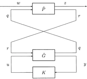
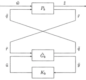
Then the closed-loop system in Fig. 1 can be decom-posed as two interconnected subsystems as follows:
Ex = (A + B2F2+ B2∆1– 1D12TR0– 1D11F1)x + (B1– B2∆1– 1D12TR0– 1D11)w + B2∆1– 1D12TR0– 1q z = (C1+D11F1+D12F2)x+q r=–F1x+w and Ex =(A+B1F1)x+B1r+B2u q=–D12F2x+D11r+D12u y=(C1+D21F1)x+D21w.
This is shown pictorially in Fig. 2, where Fig. 2 Decomposition of the closed-loop system
P = E, A + B2F2 B1– B2∆1– 1D12TR0– 1D11 B2∆1– 1D12TR0– 1 + B2∆1– 1D12TR0– 1D11F1 C1+ D11F1+ D12F2 0 I – F1 I 0 (25) and G = E, A + B1F1 B1 B2 – D12F2 D11 D12 C2+ D21F1 D21 0 .
Let x denote the state of G with respect to a given input w, and z its corresponding output. Then, by a standard game-theoretic argument, it can be shown that d dt(x TET XEx) – zTw = 1 2x TR 1(XE)x – 1 2 w – w*(x) u – u*(x) T Mw – w *(x) u – u*(x) , (26) where u* (x)=F2x, w*(x)=F1x and M = R0 R12 D12T 0 .
Integrating (26) from zero to infinity and setting x(0) =x(∞)=0 yields zT(t)w(t)dt 0 ∞ = qT(t)r(t)dt 0 ∞ (27)
Equation (27) shows that Tzw (transfer function
ma-trix from w to z) is ESPR if and only if Tqr is. This is
summarized in the following statement.
Proposition 8. Consider the standard system connec-tion (1). Suppose that the following GARE
R1(X) =∆[A – B1R0– 1C1– (B2– B1R– 10 D12)∆1– 1DT12R0– 1C1]TX + XT[A – B1R0 – 1 C1– (B2– B1R0 – 1 D12)∆1 – 1 D12 T R0 – 1 C1] + XT[B1R0– 1B1T– (B2– B1R0– 1D12)∆1– 1(B2– B1R0– 1D12)T]X + C1TR0– 1(R0– D12∆1– 1D12T)R0– 1C1= 0 , ET X=XT E
has an admissible solution XE with ETXE=XE T
E≥0. Then K internally stabilizes G and Tzw is ESPR if and
only if K internally stabilizes G and Tqr is ESPR.
The main result of this section reads as follows. Theorem 9. Consider the plant G=GSF and assume
that assumptions (A1) to (A4) are satisfied. Then there exists a state feedback controller u=Fx such that
the resulting closed-loop system is internally stable and ESPR if and only if the GARE
R1(X) =∆[A – B1R0– 1C1– (B2– B1R– 10 D12)∆1– 1DT12R0– 1C1]TX + XT[A – B1R0– 1C1– (B2– B1R– 10 D12)∆1– 1D12TR0– 1C1] + XT[B1R0– 1B1T– (B2– B1R0– 1D12)∆1– 1(B2– B1R0– 1D12)T]X + C1TR0– 1(R0– D12∆1– 1D12T)R0– 1C1= 0 , ET X=XT E has an admissible solution XE with ETXE=XE
T
E≥0, where ∆1=
∆
D12TR0– 1D12. Moreover, when this condi-tion holds, all ESPR state feedback controllers can be parameterized as K=LFT(MSF, Q), where MSF= E, A + B1F1+ B2F2 0 B2 0 F2 I – I I 0 ,
Q∈RH∞, and D11+D12Q P is ESPR with
P = E, A + B1F1+ B2F2 B1 I 0 , in which F2=∆∆1– 1D12TR0– 1(B1TXE– C1) –∆1 – 1B 2 T XE (28) F1=∆R0– 1(B1TXE– C1– D12F2) (29) ■
(i) Proof of Necessity
Suppose that u=Fx is one such controller. Us-ing this as a feedback law and closUs-ing the loop to get (see Fig. 1)
Tzw= E,
A + B2F B1 C1+ D12F D11 ,
which is internally stable and ESPR. By generalized Positive Real Lemma (Lemma 7), it follows that there exists a nonsingular matrix P satisfying the GARI
(A + B2F) T P + PT(A + B2F) + [P T B1 – (C1+ D12F)T]R0– 1[PTB1– (C1+ D12F)T]T< 0 , ETP = PTE≥ 0 .
After some algebraic manipulation, the above GARI can be rewritten in a more comapct form, i.e.
R1(P)<0, with ETP=PTE≥0. (30) We see that if the hypotheses in Lemma 4 were satisfied, then we can deduce from (30) that GARE R1(X)=0 has an admissible solution. In view of Lemma 4, we need to prove the following:
1. The pencil
– jωE + [A – B1R0– 1C1– (B2– B1R0– 1D12)∆1– 1D12TR0– 1C1] C1TR0– 1(R0– D12∆1– 1D12T)R0– 1C1
has no pure imaginary zeros.
It is easy to verify this point by assumption (A4). 2. {E, A–B1R0 – 1 C1–(B2–B1R0 – 1 D12)∆1 – 1 D12 T R0 – 1 C1} is impulse-free.
Observe the following identity, = I – (B2– B1R0 – 1 D12)∆1– 1D12TR0– 1 0 I I – B1R0– 1 0 I ⋅ – jωE + A B2 C1 D12 = – jωE + A – B1R0– 1C1 0 – (B2– B1R0– 1D12)∆1– 1D12TR0– 1C1 C1 D12
Since P1(s) is column reduced, the matrix pencil on the right side of the above identity should be column reduced as well. This implies that {E, A– B1R0 – 1 C1–(B2–B1R0 – 1 D12)∆1 – 1 D12 T R0 – 1 C1} is im-pulse-free. This completes the proof of necessity. (ii) Proof of Sufficiency
Suppose now that the GARE R1(X)=0 has an ad-missible solution XE. Motivated by Proposition 8,
we first make a change of variables defined as (21) which we reproduce here for the sake of clarity.
r=∆w–F1x
q=∆D11r+D12(u–F2x).
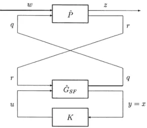
Then the closed-loop system in Fig. 1 with G=GSF
can be decomposed as two interconnected subsystems as follows: Ex = (A + B2F2+ B2∆1 – 1 D12 T R0 – 1 D11F1)x + (B1– B2∆1 – 1 D12 T R0 – 1 D11)w + B2∆1 – 1 D12 T R0 – 1 q z=(C1+D11F1+D12F2)x+q r=–F1x+w and Ex =(A+B1F1)x+B1r+B2u q=–D12F2x+D11r+D12u y=x.
This is shown pictorially in Fig. 3, where
Fig. 3 Decomposition of the closed-loop system in state feedback case
and GSF= E, A + B1F1 B1 B2 – D12F2 D11D12 I 0 0 . Set K= EK, AK BK CK 0
. Then the dynamical equa-t i o n s f o r equa-t h e l i n e a r f r a c equa-t i o n a l equa-t r a n s f o r m a equa-t i o n LFT(GSF, K) are: LET(GSF, K) = E 0 0 EK , A + B1F1 B2Ck B1 BK AK 0 – D12F2 D12CK D11 =∆ E, A B C D ,
and the dynamical equations for the closed-loop sys-tem LFT(GSF, K) are LFT(GSF, K) = LFT(P, LFT(GSF, K)) = ∆ EC, AC BC CCDC where AC= A + B2F2 AC 1 AC 2 A with AC1=[–B2F2 B2CK] and AC2= – B1F1 0 , BC= B1 B , CC = [C1+ D12F2 C] , and DC=D11, EC= E 0 0 E Let ∆ =∆ DT+ D and ∆C=∆DC T +DC. It is easy to
see that ∆=DC=R0>0. Now using equations Eqs. (28) and (29), it is straightforward but tedious to verify that, with XC= ∆ XE 0 0 X for some X, RC(XC) = ∆ (AC– BC∆C– 1CC) T XC+ XC T (AC– BC∆C– 1CC) + CC T ∆C– 1CC + XC T BC∆C– 1BC T XC = R1(XE) 0 0 R(X) where R(X) =∆(A – B∆– 1C)TX + XT(A – B∆– 1C) + CT∆– 1C + XTB∆– 1BTX .
Furthermore, it is straightforward to verify that
AC– BC∆C – 1 CC + BC∆C – 1 BC T XC = A + B1F1+ B2F2 * 0 A – B∆– 1C + B∆– 1BTX where the ‘*’ stands for an irrelevant entry. Hence, using the fact that XE is an admissible solution to the
GARE R1(X)=0 together with Proposition 8, we can conclude that XC is an admissible solution to the
GARE RC(XC)=0 if and only if X is an admissible
solution to the GARE R(X) =0, and, in addition, EC T XC=XC T EC≥0 if E T X = XTE≥0. Then K internally stabilizes GSF and Tzw is ESPR if K internally
stabi-lizes GSF and Tqr is ESPR. The rest of the proof is
P = E, A + B2F2 B1– B2∆1 – 1 D12 T B0– 1D11 B2∆1 – 1 D12 T R0– 1 + B2∆1– 1D12TR0– 1D11F1 C1+ D11F1+ D12F2 0 I – F1 I 0 (31)
then to find all internally stabilizing K for GSF such
that Tqr is ESPR.
Take an admissible realization of Q:
Q = EQ,
AQBQ
CQDQ
.
Since Q∈RH∞, {EQ, AQ} is admissible. Note that the
dynamical equations for D11+D12QP are E 0 0 EQ , A + B1F1+ B2F2 0 B1 BQ AQ 0 D12DQ D12CQ D11 =∆ E, A B C D .
The fact that {E, A+B1F1+B2F2} is admissible implies that { E , A } is also admissible. Together with the hypothesis that D11+D12QP, is ESPR, it fol-lows from Lemma 7 that there exists a matrix X which satisfies the GARE
( A – B R0– 1C )TX + XT( A – B R0– 1C ) + CTR0– 1C + XTB R0– 1B TX = 0 , ETX = X TE ,
with E TX = XTE >0 and is such that the matrix pair {E , A – B R 0– 1C + B R0– 1B TX } is admissible. The dynamical equations for the closed-loop system are: LFT(GSF, K)=LFT(GSF, LFT(MSF, Q)) = E 0 0 0 E 0 0 0 EQ , A + B2F2 – B2DQ B2DQ B1 + B2DQ B2DQ A + B1F1+ B2F2 B2DQ 0 – B2DQ BQ – BQ AQ 0 C1+ D12F12 – D12DQ D12DQ D11 + D12DQ . A p p l y a n e q u i v a l e n t t r a n s f o r m a t i o n w i t h M= I 0 0 I – I 0 0 0 I
on the left and N=M–1
on the right to the
last realization to get
LFT(GSF, K) = E ° , A° B° C°D° , where E°= E 0 0 0 E 0 0 0 EQ A°= A + B2F2 A1° A2° A with A1°= [B2DQ B2DQ] and A2°= – B1F1 0 , B°= B1 B , C ° = [C1+ D12F2 C ] and D°= D = D11
Then it can be shown by a routine calculation that the matrix
X°=∆ XE 0 0 X
satisfies the GARE (A°– B°R0– 1C°)TX°+ X°T(A°– B°R0– 1C°) + C°TR0– 1C°+ X°TB°R0– 1B°TX°= 0 , E°TX°= X°TE°, (32) with E°T X°=X°T E°≥0. Moreover, it is straightforward to show that the matrix pair
{E°, A – B°R0 – 1 C°+ B°R0 – 1 B°TX°} = E 0 0 E , A + B1F1 * + B2F2 0 A – B R0– 1C + B R0– 1B TX
is admissible. Hence, X° is an admissible solution to the GARE (32). It now follows from Generalized Positive Real lemma that the controller K=LFT(MSF,
Q) for any given Q∈RH∞ with D11+D12QP ESPR does internally stabilize GSF and render the closed-loop
system ESPR.
To complete the proof, we need to show that for any given state feedback controller K that achieves closed-loop internal stability and ESPR can be ex-pressed in the form of LFT(MSF, Q) for some Q∈RH∞
with D11+D12QP ESPR. Now introduce
MSF= ∆ E, A + B1F1 – B2F2 B2 – F2 – F2 I I I 0 .
Then K internally stabilizes MSF since K internally
stabilizes GSF by Proposition 8. Thus LFT(MSF, K)
∈RH∞. Let Q =∆ LFT(M
SF, K)∈RH∞. Then it can be
shown after some algebraic manipulation that D11+D12QP=LFT(GSF, K). Again, it follows from
Proposition 8 that D11+D12QP is ESPR. Moreover, it is straightforward to verify that LFT(MSF, Q)=LFT
(MSF, LFT(MSF, K))=LFT(NSF, K), where NSF= E 0 0 E , A + B1F1+ 2B2F2 – B2F2 – B2F2 B2 B2F2 A + B1F1 – B2F2 B2 F2 – F2 0 I – I I I 0 .
Conjugating the states of NSF by
I 0 – I I on the left and I 0 – I I – 1 = I 0
I I on the right yields
NSF= E 0 0 E , A + B1F1 – B2F2 – B2F2 B2 + B2F2 0 A + B1F1 0 0 + B2F2 0 – F2 0 I 0 I I 0 = 0 I I 0 .
Thus LFT(MSF, Q)=LFT(NSF, K)=K. This completes
the proof.
Remark. The parameter Q above is governed by an ESPR-like constraint. The weighting matrices D12 and P can be eliminated by multiplying certain ma-trix inverses as described in Zhou (1996) which gives all state feedback controllers for H∞ control problem. N e v e r t h e l e s s , t h e i n f l u e n c e o f D1 1 c a n n o t b e eradicated.
IV. ESPR OUTPUT FEEDBACK CONTROL PROBLEM
1. Central Controller
Before proceeding to the main problem of this paper, we need a preliminary result which is stated in the following theorem.
Theorem 10. Consider the standard system connec-tion (Fig. 1) with
Ex =Ax+B1w+B2u G=GFI= ∆ z=C1x+D11w+D12u, y = x y .
Suppose that assumption (A1) to (A4) hold. Then the ESPR full information control problem for de-scriptor systems is solvable if and only if the GARE R1(X)=0 has an admissible solution XE with ETXE=
XE T
E≥0. Moreover, if this condition is satisfied, one such controller is given by u=[F2 0]y. ■ Remark. The proof is pretty similar to the proof of Theorem 9 and is, thus, omitted. Note that the as-sumption (A1) can be replaced by a weaker one. We will not pursue this point here.
The following theorem provides a the necessary and sufficient condition for the solvability of ESPR output feedback control problem.
Theorem 11. Consider the standard system connec-tion (Fig. 1) with G=GOF. Suppose that assumptions
(A1) to (A7) hold. Then the following statements are equivalent.
(I) There exists a controller of the form (2) such that the resulting closed-loop system is internally stable and ESPR.
(II) (i) the GARE R1(X)=0 has an admissible solu-tion XE with ETXE=XE
T
E≥0. (ii) the GARE
R3(Z) =∆AZZ + Z T AZ T – ZT(C2ZT ∆2– 1C2Z– F2T∆1F2)Z + B1ZR0– 1B1ZT = 0 , EZ = ZTET
has an admissible solution ZE with EZE=
ZE T ET≥0, where ∆2= ∆ D21R0– 1D21T AZ= ∆ A + B1R0– 1(B1TXE– C1) – B1R0 – 1 D21T∆2– 1C2Z B1Z=∆B1(I – R0– 1D21T∆2– 1D21) C2Z=∆C2+ D21R0– 1(B1TXE– C1)
Moreover, when these conditions are satisfied, one such controller is given as in the form (2) with
E0= E A0= A + B2C0– B0C2 + (B1– B0D21)R0– 1(B1TXE– C1– D12C0) B0= (ZE T C2Z T + B1R0 – 1 D21 T )∆2– 1 C0= F2 ■
Before giving the proof of the theorem, we note that the hierarchically coupled pair of GAREs given above can be further manipulated to yield two mutually decoupled GAREs, with a separated additional spec-tral radius condition. This is summarized in the fol-lowing statement.
Corollary 12. Suppose that GARE R1(X)=0 has an admissible XE with ETXE=XE
T
E≥0. Suppose also that the following conditions are satisfied.
(i) The GARE R2(Y) = ∆ [A – B1R0 – 1 C1– B1R0 – 1 D21 T ∆2 – 1 (C2– D21R0 – 1 C1)]Y + YT[A – B1R0– 1C1– B1R0– 1D21T∆2– 1(C2– D21R0– 1C1)]T + YT[C1TR0– 1C1– (C2– D21R0– 1C1)T∆2– 1(C2– D21R0– 1C1)]Y + B1R0 – 1 (R0R21 T ∆2 – 1 D21)R0 – 1 B1 T = 0 EY=YT ET ,
has an admissible solution YE with EYE=YE T
ET≥0 (ii) The Spectral Radius ρ(YE, XE)<1
Then the condition (II) of Theorem 11 holds.
Moreover, when these conditions are satisfied, the m a t r i c e s XE, YE a n d ZE h a v e t h e f o l l o w i n g
relationship:
ZE=(I–YEXE)–1YE=YE(I–XEYE)–1. ■
Remark. This corollary is easily verified by involv-ing some simple algebraic calculations. Unlike the LTI case [7], this result is, in general, not a neces-sary and sufficient condition since the matrix I+XEZE
may not be invertible.
(i) Proof of Sufficiency of Theorem 11
Observe that the closed-loop system (1)-(2) can be written as εC xe = AC xe + BCw z = CC xe + DCw where εC = ∆ E 0 0 E0 AC= ∆ A + B2C0 – B2C0 A – A0+ B2C0– B0C2 A0– B2C0 BC= ∆ B1 B1– B0D21 CC= ∆ [C1+ D12C0 – D12C0] DC= ∆ D11 and e=∆x – x0
The GARE R3(Z)=0 can be rewritten as: R3(Z) = ( AZ– BZR0 – 1 CZ)Z + Z T ( AZ– BZR0 – 1 CZ) T + BZR0 – 1 BZ T + ZTCZ T R0– 1CZZ = 0 , EZ=ZT ET where AZ= ∆ AZ– ZE T C2ZT∆2– 1C2Z+ BZR0 – 1 CZ BZ= ∆ B1Z– ZE T C2z T ∆2 – 1 D21 CZ= ∆ R01/2∆11/2F2
Note that ZE is also the admissible solution to GARE
(33).
By Generalized Positive Real Lemma, we can conclude that {ET , A Z T } is admissible and BZ T (sET – AZ T )–1C Z T
+D11T is ESPR. This, in turn, implies that {E, AZ } is admissible and CZ (sE–AZ )–1BZ +D11 is ESPR.
Again by Generalized Positive Real Lemma, the GARE R4(W) = ( AZ– BZR0 – 1 CZ) T W + WT( AZ– BZR0 – 1 CZ) + CZ T R0– 1Cz+ W T BZR0 – 1 BZ T W = 0 ET W=WT E
has an admissible solution WE with ETWE=WE T E≥0. Now Set PC= ∆ XE 0 0 WE . Clearly, EC T PC= PC T
EC. Lengthy but otherwise
rou-tine calculation shows that PC is an admissible
solu-tion to the GARE AC T P + PTAC+ (P T BC– CC T )R0– 1(PTBC– CC T )T= 0 , εCTP = P T εC with εCT P C= PC T
εC≥0. It follows, again from
Gener-alized Positive Real Lemma, that (2) is a stabilizing controller such that Tzw is ESPR. This completes the
proof of sufficiency.
(ii) Proof of Necessity of Theorem 11
Suppose that KOF is one solution. Then the
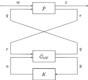
con-troller KFI=KOF[C2 D21] solves the FI problem. From Theorem 10, it follows that GARE R1(X)=0 has an admissible solution. Consequently, we see that F1, F2 are well defined. As in the state feedback case, we shall make a change of variables described by (21). Then by a similar argument as in the proof of Theo-rem 9, the closed-loop system in Fig. 1 can be de-composed as two interconnected subsystems. This is illustrated in Fig. 4, where P is given as in (31) and
GOF= E, A + B1F1 B1 B2 – D12F2 D11 D12 C2+ D21F1 D21 0 .
Since the GARE R1(X)=0 has an admissible
solution XE with ETXE=XE T
E≥0, then, by Proposition 8, K internally stabilizes GOF and Tzw is ESPR if and
only if K internally stabilizes GOF and Tqr is ESPR.
The rest of the necessity proof follows by observing first that K internally stabilizes GOF and Tqr is ESPR
if and only if KT internally stabilizes GOF T and Tqr T is ESPR. Now introduce
Gb= ∆ GOF T = ET, (A + B1F1) T – F2 T D12 T (C2+ D21F1) T B1T D11T D21T B2T D12T 0 =∆ E, A B1 B2 C1 D11 D12 C1 D21 0 .
As a consequence of Proposition 8 and the above observation, the ESPR OF problem for Gb is also
solvable. Again, suppose that Kb solves the ESPR
OF problem for Gb then the controller Kb=[C2 D21] solves the FI problem inherited from Gb. It follows,
again from Theorem 10, that GARE R1(X) =∆[A – B1R0– 1C1– (B2– B1R– 10 D12)∆1– 1DT12R0– 1C1]TX + XT[A – B1R0– 1C1– (B2– B1R– 10 D12)∆1– 1D12TR0– 1C1] + X[B1R0– 1B1T– (B2– B1R0– 1D12)∆1– 1(B2– B1R0– 1D12)T]X + C1TR0– 1(R0– D12∆1– 1D12T)R0– 1C1
Fig. 4 Decomposition of the closed-loop system in output feed-back case
ETX = XTE
has an admissible solution X with ETX =XTE≥0 where R0=D11 T +D11=R0 and ∆1=D12 T R0 – 1 D12=∆2. It is easy to verify that R1(X) is exactly R3(X). This shows that
X =∆ZE indeed exists. This completes the necessity
proof.
2. Characterization of All ESPR Output Feedback Controllers
The following theorem, which is the main re-sult of this section, characterizes all output feedback controllers that achieve closed-loop internal stability and ESPR
Theorem 13. Suppose that assumptions (A1) to (A7) are satisfied. Suppose also that condition (II) of Theorem 11 holds. Then the set of all output feed-back controllers that achieve closed-loop internal sta-bility and ESPR can be parameterized as K=LFT (MOF, Q), where MOF= E, A0 B0 B1 C0 0 I – (C2+ D21F1) I 0 ,
A0, B0, C0 are defined as in Theorem 11, B1= ∆ (I + XEZE) T (B2– B1R0 – 1 D12) + (C1ZE+ D21 T B0T)TR0– 1D12 (34) Fig. 5 Block diagram for LFT(Gb, Kb)
Fig. 6 Decomposition of LFT(Gb, Kb)
and Q∈RH∞ with D11+D12Q D21 ESPR. ■ Proof. From subsection (ii), the problem of param-eterizing all internally stabilizing controllers for GOF
such that Tzw is ESPR is equivalent to the problem of
parameterizing all internally stabilizing controllers Kb
for Gb such that Tqr T
is ESPR. In what follows, we shall focus on the problem of parameterization of all internally stabilizing controllers Kb for Gb such that
Tqr T
is ESPR. Denote by x , {w , u } and {z , y } the state, inputs and outputs of Gb, respectively, as shown
in Fig. 5. Next, make a change of variables as follows:
r =∆w – F1x q =∆D11r + D12(u – F2x) where F1=∆R0– 1(B1TX – C1– D12F2) F2=∆∆1– 1D12TR0– 1(B1TX – C1) –∆1– 1B2TX .
Then it follows, by direct verification using the same arguments as before, that the closed-loop system in Fig. 5 can be decomposed as two interconnected subsystems. This is shown pictorially in Fig. 6, where
Pb= E, A+ B2F2 B1– B2∆1– 1D12TR0– 1D11 B2∆1– 1D12TR0– 1 + B2∆1– 1D12TR0– 1D11F1 C1+ D11F1+ D12F2 0 I F1 I 0
and Gb= E, A + B1F1 B1 B2 – D12F2 D11 D12 C2+ D21F1 D21 0 .
Again, applying Proposition 8 shows that Kb
inter-nally stabilizes Gb and Tqr
T
=Tzw is ESPR if and onlyif Kb internally stabilizes Gb and Tqr is ESPR.
Now let L=∆F2T=C0T, then simple algebra shows that {E, A+B1F1+L(C2+D21F1)}={ET, (A+B1F1+ B2F2)T which is admissible. Also note that if we let F=∆–B0T, then it is straightforward to verify that {E, A+B1F1+B2F}={ET, AZ
T
–C2ZT∆2– 1C2ZZE+F2
T
∆1F2ZE},
which is also admissible since ZE is an admissible
so-lution to R3(Z)=0. Then, from Theorem 2 of Wang, H. S. et al. (1997), all internally stabilizing control-lers for Gb can be parameterized as Kb = LFT(Mb,
Qb) with Qb∈RH∞, where Mb= E, A + B1F1– B2B0T – C0T B2 + C0T(C2+ D21F1) – B0T 0 I – (C2+ D21F1) I 0 .
It is easy to see that Mb can be rewritten as
Mb= E, A0T – C0T (C2+ D21F1)T – B0T 0 I – B1T I 0 , where B1 is as defined by (34).
Moreover, a little bit of algebra shows that Tqr= LFT(Gb, LFT(Mb, Qb)) = D11 T + D21TQbD12 T . So Tqr is ESPR if and only if D11
T
+D21T QbD12
T
is ESPR.
Thus all internally stabilizing controllers for GOF
T
such that Tqr T
is ESPR can be parameterized as Kb= L F T ( Mb, Qb) , w h e r e Qb∈RH∞ w i t h D11
T
+ D21T QbD12
T
ESPR. Consequently, all internally stabi-lizing controllers for GOF such that Tqr is ESPR can
be parameterized as K=Kb T =LFT(Mb T , Q) where Q=∆Qb T ∈RH∞ with D 11+D12QD21 ESPR. It is easy to see that Mb T
=MOF. This completes the proof. Q.E.D.
The parametrization given above is an implicit one. We leave this form here for the readers’ sake of comparision with the SF parametrizaton. However,
the parametrization can be explicitly defined via simple algebraic manipulations.
Theorem 14. Suppose that assumptions (A1) to (A7) are satisfied. Suppose also that condition (II) of Theorem 11 holds. Then the set of all output feed-back controllers that achieve closed-loop internal sta-bility and ESPR can be parameterized as K=LFT (Mb T OF, G), where MOF= E, A0– B1D12– L B0+ B1D12– L B1D12– L ⋅ D11(D21 – R + F1) ⋅ D11D21– R – C0– D12– LD11 D– L12D11D21– R D12– L ⋅ (D21 – R + F1) – (D21– RC2+ F1) D21– R 0 ,
with Q ESPR, where D12– L and D21– R denote any left and right inverses of D12 and D21, respectively. ■
Proof. The proof is fairly straightforward, thus omitted.
V. CONCLUSION
In this paper, we have given the descriptor for-mulations of all state feedback and output feedback controllers, respectively, that achieve closed-loop internal stability and ESPR. We have also investi-gated some properties of the GARE. The ESPR con-trol problem for which D11+D11
T
>0 (assumption (A1)) is examined. (A1) is a necessary condition for an ESPR problem to be solvable in the usual linear time-invariant case; but, quite the contrary, this is no longer the case for the descriptor systems.
As a bottleneck of the quadratic optimization problems, we believe it is time for us to survey some properties of the generalized algebraic Riccati equation. In this paper, we have recovered some prop-erties of the coupled GARE (3) and GARI (4). It’s seen that GAREs have a property similar to the mono-tonicity of AREs: If X is an admissible solution of a GARE and P is a solution of the GARI deduced from the GARE, then, xT
ET Px–xT
ET
Xx>0 for all x∈ℑmE. Parameterization of all output feedback control-lers is via the Youla parameterization for descriptor systems. The parameterization is given in an explicit form; but this is not the situation for the state feed-back parameterization. We see that state feedfeed-back controllers have no influence on “D11w” term; hence, it is reasonable that the constraint on Q should in-volve the D11 matrix.