Lower Bounds for Asian Options

國立台灣大學財務金融研究所碩士論文

指導教授 ： 呂育道 博士

算術平均式亞式選擇權之價格下限

Lower Bounds for

Asian Options

研究生：陳冠文 撰

中華民國九十四年六月

Lower Bounds for

Asian Options

Kuan-Wen Chen

Department of Finance

National Taiwan University

Table of Contents

1 Introduction

1.1 Background

1.2 Structures of the Thesis

2 Mathematical Preliminaries

2.1 Correlation Matrices

2.2 Basic Statistical Properties

3 Lower Bounds

3.1 Fixed-Strike Asian Options

3.2 Floating-Strike Asian Options

4 Numerical Results

4.1 Numerical Results

5 Conclusions and Future Work

Appendix

Proof for Theorem A.1 Proof for Theorem A.2

Bibliography

Abstract

There are two types of Asian options, fixed-strike and floating-strike, in the literature. We give lower bounds on the values of both fixed-strike and floating-strike Asian options in continuous case. Good lower bounds for both options have been derived earlier by Rogers & Shi (1995) and Thompson (1998). But the lower bound derived by Thompson assumes a maturity of one year. This thesis extends Thompson’s version of the lower bound to the case of general maturities. Numerical experiments are performed to confirm the extreme accuracy of the lower bound.

Chapter 1

Introduction

1.1 Background

Fixed-strike Asian (call) options are options whose payoff depends on the average price of the underlying asset during at least some part of the life of the option. The payoff

from a fixed-strike Asian call is , where is the

average value of the underlying asset calculated over a predetermined averaging period, is called the strike price or the exercise price, and

ave S

0 >

K T is the maturity date. We

assume that the asset price follows a geometric Browning motion S_t =Sexp(σB_t +αt),

where 2

2 1_σ

α = r− is a constant, r is the risk-free interest rate (assumed to be a

constant), S is the stock price, σ is the volatility, and B_t is a Browning motion.

0 1 max(0 , S_ave K) TS dt K_t T + ⎛ ⎞ − =_⎜ − _⎟ ⎝

∫

⎠

Another type of Asian (call) option is the floating-strike Asian (call) option. The

payoff is 0 1 max(0 , S_ave S_T) TS dt S_{t T} T + ⎛ − =_⎜ − ⎝

∫

⎠ ⎞

⎟ , where is the stock price at the

maturity date.

T

S

Exact analytic formulas for Asian options don't exist. This is primarily due to the fact that the arithmetic average of a set of lognormal random variables has a distribution that

is largely intractable. Then several approaches to the problem of valuing Asian options have been put forward in the literature:

1. Monte-carlo simulation: Boyle (1977) and Kemna & Vorst (1990) and Corwin & Boyle & Tan (1996).

2. Binomial tree method: Hull & White (1993) and Neave & Turnbull (1993). 3. Convolution method: Carverhill & Clewlow (1990).

4. Triple integral: Yor (1992) and Geman & Yor(1993).

5. Partial derivative equation (PDE): Dewynne & Wilmott (1995) and Alziary & Decamps & Koehl (1997).

6. Fast fourier transform (FFT): Caverhill and Clewlow (1992) and Benhamou (2002).

7. Approximation method: Turnbull & Wakeman (1991) and Levy (1992) and Vorst (1992) and Milevsky & Posner (1998) and Curran (1992) and Rogers & Shi (1995) and Thompson (1998).

In this thesis, we consider analytical approximation methods. They are easier to evaluate.

Thompson (1998) assumes T =1 (year). In this thesis, we extend his result to the general case of T =τ years.

1.2 Structures of the Thesis

There are five chapters in this thesis. In Chapter 2, we introduce some useful Mathematical Preliminaries for later analysis. In Chapter 3, we introduce lower bounds to the case of general maturities. In Chapter 4, we present the numerical results.

Chapter 2

Mathematical Preliminaries

2.1 Correlation Matrices

Like most of the approximation formulas in the literature, we need the correlation matrix between B ds T T s

∫

0 1 and B_t. Theorem 2.1

The correlation matrix between B ds

T T s

∫

0 1 and B_t equals 0 0 0 0 1 Cov( , ) Cov , 2 1 1 1 Cov , Cov , 2 3 T t t t s T T T t s s s t t B B B B ds t T T T t t T B B ds B ds B ds T T T T T ⎡ ⎛ ⎞ ⎤ ⎡ ⎛ ₋ ⎞⎤ ⎜ ⎟ ⎜ ⎟ ⎢ _{⎝ ⎠} ⎥ ⎢ _{⎝ ⎠}⎥ ⎢ ⎥ ⎢₌ ⎥ ⎢ _{⎛ ⎞ ⎛ ⎞}⎥ ⎢ _{⎛ ⎞} ⎥ − ⎢ ⎜ ⎟ ⎜ ⎟⎥ ⎢ ⎜ ⎟ ⎥ ⎝ ⎠ ⎝ ⎠ ⎝ ⎠ ⎣ ⎦ ⎣ ⎦

∫

∫

∫

∫

where 0<t <T. Proof:

(i) Cov(B_t , )B_t =Var(B_t)= by the definition of Brownian motion. t

(ii) 0 0 0 0 1 1 1 1 Cov B_t , TB ds_s E B_t TB ds_s E B E( _t) TB ds_s E TB B ds_{t s} T T T T ⎛ ⎞₌ ⎛ _⋅ ⎞₋ ⎛ ⎞₌ ⎛ _⋅ ⎞ ⎜ ⎟ ⎜ ⎟ ⎜ ⎟ ⎜ ⎟ ⎝

∫

⎠ ⎝

∫

⎠ ⎝

∫

⎠ ⎝

∫

⎠ 0 0 1 1 1 ( ) ( ) ( ) T t T t s t s _t t s E B B ds E B B ds E B B ds T T T =

∫

⋅ =

∫

⋅ +

∫

⋅ = 2 0 1 1 1 ( ) 2 2 t T t t t s ds t ds t T t T T T T T ⎛ ⎞ _{⎛ ⎞} + = _⎜ + − _⎟= _{⎜ ⎟} ⎝ ⎠ ⎝ ⎠

∫

∫

−t .

(iii) ₂

(

)

0 0 0 0

1 1 1 1

Cov TB ds_s , TB ds_s Var TB ds_s Var TB ds_s

T T T T

⎛ ⎞₌ ⎛ ⎞₌

⎜ ⎟ ⎜ ⎟

⎝

∫

∫

⎠ ⎝

∫

⎠

∫

.

By Hoel, Port, and Stone (1986),

(

)

(

)

2 Var b ( )( _{t a}) ( )b ( ) a f t B′ −B dt = a f t − f b dt

∫

∫

. So

(

)

2 2 ₀ 2 ₀ 1 1 Var ( ) 3 T T s T B ds s T ds T

∫

=T

∫

− = . Theorem 2.2

The correlation matrix between TB_sds B_T T

∫

0 − 1 and B_t equals 2 0 2 0 0 0 1 Cov( , ) Cov , 2 1 1 1 Cov , Cov , 2 3 T t t t s T T T T t s T s T s T t B B B B ds B _t T _T t T B B ds B B ds B B ds B T T T T ⎡ ⎛ ₋ ⎞ ⎤ ⎡ − ⎤ ⎜ ⎟ ⎢ _{⎝ ⎠ ⎥ ⎢ ⎥} ⎢ _{⎥ ⎢}= ⎥ ⎢ ⎛ ₋ ⎞ ⎛ _{− −} ⎞⎥ ⎢− ⎥ ⎢ ⎜_⎝ ⎟_⎠ ⎜_⎝ ⎟_⎠⎥ ⎢_⎣ ⎥_⎦ ⎣ ⎦

∫

∫

∫

∫

where 0<t <T. Proof: (i) 0 0 0 1 1 1 Cov B_t , TB ds B_{s T} E B_t TB ds B_{s T} E B E( _t) TB ds B_{s T} T T T ⎛ ⎞ ⎛ ₋ ⎞_{= ⋅}⎛ ₋ ⎞ ₋ ⎛ ₋ ⎜ ⎟ ⎜ ⎜ ⎟⎟ ⎜ ⎝

∫

⎠ ⎝ ⎝

∫

⎠⎠ ⎝

∫

⎞ ⎟ ⎠ 2 0 0 1 1 ( ) ( ) 2 2 T T t s T t s t t E B B ds B E B B ds t T t T T T ⎛ ⎛ ⎞⎞ − = _⎜ ⋅_⎜ − _⎟⎟= ⋅ − = − − = ⎝ ⎠ ⎝

∫

⎠

∫

t T . (ii)

(

)

2 0 0 0 0 1 1 1 1

Cov TB ds B_{s T} , TB ds B_{s T} Var TB ds B_{s T} Var TB ds B_{s T}

T T T T ⎛ _{− −} ⎞₌ ⎛ ₋ ⎞₌ ⎜ ⎟ ⎜ ⎟ ⎝

∫

∫

⎠ ⎝

∫

⎠

∫

−

(

)

(

)

{

}

3 2 _{0 0} 2 1 1

Var Var( ) 2Cov , 2

3 2 T T s T s T T T B ds B B ds B T T T ⎧ ⎫ = + − = _⎨ + − _⎬ ⎩ ⎭

∫

∫

=T₃ .

2.2 Basic Statistical Properties

Definitions

Let −∞<µ_x <∞, −∞<µ_y <∞, 0<σ_x, 0<σ_y and −1<r<1 be real numbers. The bivariate normal PDF (probability density function) with means µ_x and

y

µ , variances 2 and , and correlation x

σ 2

y

σ ρ is the bivariate PDF given by

for −∞< x<∞ and −∞< y<∞, and uaually denoted by φ

(

µ_x,µ_x, σ_x2, σ_y2 ,ρ

)

2 2 2 2 1 1 ( , ) exp 2 2(1 ) 2 1 y y x x x x y y x y y y x x f x y µ ρ µ µ µ ρ σ σ σ σ πσ σ ρ ⎛ ₋ ⎧_{⎪⎛ − ⎞ ⎛ − ⎞⎛ − ⎞ ⎛ − ⎞} ⎫_⎪⎞ ⎜ ⎟ = _{⎜ −} ⎨⎜ ⎟ − ⎜ _⎟⎜⎜ ⎟ ⎜_{⎟ ⎜}+ ⎟_⎟ ⎬_⎟ − _⎝ ⎪_⎩⎝ ⎠ ⎝ ⎠⎝ ⎠ ⎝ ⎠ ⎪_⎭⎠ Theorem 2.3

If bivariate normal random variable

(

X Y,

)

~φ

(

µ_x ,µ_x,σ_x2 ,σ2_y ,ρ

)

, the conditional distribution of X given Y = is normal with mean y

(

_x

)

y x x _σ y µ ρσ µ + − and variance 2

(

2

)

1 ρ σx − .

Proof: See Sheldon Ross (1998).

By Theorem 2.3, if X =B_t and B ds T

Y =

∫

T _s

0

1

, then the conditional

distribution of B_t given B ds z T T s =

∫

0 1

is normal with mean 3

(

₂/2

)

T z t T t − and

variance 2 3 2 2 3 ⎟ ⎠ ⎞ ⎜ ⎝ ⎛ − − T t T t

t , and the conditional distribution of B_t given

x B ds B T T T s − =

∫

0 1

is normal with mean ₂

2 2 3 T x t − and variance 4 3 3 4 T t t− . Definitions

The MGF (moment generating function) M_X

( )

A of the random variable X is defined for all real values of A by

( )

A E

[ ]

e e f

( )

x dx M AX Ax X

∫

∞ ∞ − =

= if X is contimuous with density f

( )

x .

Theorem 2.4

The MGF MX( A) of the random variable X ~φ

(

µ , σ2

)

is

( )

1 2 2 ( ) exp 2 AX X M A =E e = ⎛_⎜µA+ σ A ⎝ ⎠ ⎞

⎟ for all real value of A. Proof: See Sheldon Ross (1998).

Theorem 2.5

Suppose we are given two random variables X ,Y with X ~φ

(

µx,σx2

)

and

(

_, 2

)

~ _{y y} Y φ µ σ . Then

(

(

)

)

_⎟⎟ ⎠ ⎞ ⎜ ⎜ ⎝ ⎛ + Φ = > + y y u X_{I Y e} c e E x x σ µ σ2 2 1

0 , where Φ

( )

⋅ is the normal

distribution function ,I(⋅) is the indicator function and c=Cov

(

X , Y .

)

Proof: See Appendix.

Theorem 2.6

For any random variable X with density f_X

( )

x , we have (i)E

[

(

S_t −K

) (

I X >γ

)

] [

=E S_t −K;X >γ

]

; (ii)

(

)

E

(

S K X

)(

f x

)

dt T dt X K S E T T X t T t

∫

∫

− > = − = − ∂ ∂ 0 0 | 1 ; 1 _{γ γ} λ

( )

.

Chapter 3

Lower Bounds

3.1 Fixed-Strike Asian Options

Let 0 1 : T _t A S dt K T ω ⎧ ⎫ =_⎨ > _⎬ ⎩

∫

⎭. Then 0 0 0 0 0 0 1 1 1 ( ) ( ) ( ) 1 1 1 ( ) ( ) ( ) ( ) ( ) ( ) T T T t t t T T T t t t E S dt K E S dt K I A E S K dt I T T T E S K I A dt E S K I A dt E S K I A T T T + ⎧ ⎫ _{⎧ ⎫ ⎧} ⎪⎛ ₋ ⎞ ⎪₌ ⎛ ₋ ⎞ ₌ ⎛ ₋ ⎞ ⎨_⎝⎜ ⎟_⎠ ⎬ ⎨_⎝⎜ _⎠⎟ ⎬ ⎨⎜_⎝ ⎟_⎠ ⎩ ⎭ ⎩ ⎪ ⎪ ⎩ ⎭ ⎧⎛ ⎞⎫ _′ = _⎨⎜ − _⎟⎬= − ≥ − ⎝ ⎠ ⎩ ⎭

∫

∫

∫

∫

∫

∫

A dt ⎫ ⎬ ⎭

If we replace event A with another eventA′, we no longer have equality (see the illustration below). A A' A A_I ′ ' A A− 0 ' 1 : T _t A A S dt K T

ω

, − ⎧ ⎫ =_⎨ < _⎬ ⎩

∫

⎭

At this part, the integral is negative We will use A :1 TB dt_t T ω γ ⎧ ⎫ ′ =_⎨ > _⎬ ⎩

∫

0 ⎭.

We now determine the value of γ that maximizes

(

) ( )

0

1 T t

E S K I A dt

T

∫

− ′ . Note

for any random variable X with density f_X

( )

x ,

(

)

(

)(

0 0 1 1 ; | ( ) T T t t E S K X dt E S K X f x dt T γ T γ λ ∂ − > = − = − ∂

∫

∫

X

)

.

Thus the optimal value of γ , γ*, satisfies 0 1 ( | ) T t E S K X dt K T

∫

− =γ = .

With our choice of =

∫

TB_tdt T X 0 1 , we conclude that 2 * 2 2 2 3 0 1 3 ( / 2) 3 exp 2 2 T t T t t t S t t T T T T γ σ _α σ ⎧ ₋ ⎛ ⎞⎫ ⎪ _{+ + −} ⎛ ₋ ⎞ ⎪_dt=K ⎜ ⎟ ⎨ _⎜ ⎜ ⎟ _⎟⎬ ⎝ ⎠ ⎪ ⎝ ⎠⎪ ⎩ ⎭

∫

which determines γ*uniquely. We now have the bound

(

)

⎭ ⎬ ⎫ ⎩ ⎨ ⎧ ⎥ ⎦ ⎤ ⎢ ⎣ ⎡ ⎟ ⎠ ⎞ ⎜ ⎝ ⎛ _> − ≥ − ×

_∫

+

_∫

_{Bds dt} T I K Se E T e V T r T B t T _s fixed ₀ t * 0 1 1 σ α _γ .

where Φ is the normal distribution function. With , ,

, * 2 =−γ u t 2 2 1 σ σ = 3 2 2 T = σ , ) 2 (T t T t c=σ − , we have

It remains to calculate the expectation. Fix t∈

(

0,T

)

and let N₁ =σB_t +αt+logS and

* 0 2 1 _γ − =

∫

TB_tdt T N . Write u_i =E(N_i), 2 and Var( ) i Ni σ = c=Cov(N₁ , N₂). Then

(

)

(

)

[

]

_⎟⎟ ⎠ ⎞ ⎜⎜ ⎝ ⎛ Φ − ⎟⎟ ⎠ ⎞ ⎜⎜ ⎝ ⎛ + Φ = > − + 2 2 2 2 2 1 2 2 1 1 1 ₀ σ σ σ _u K c u e N I K e E N u S t u₁=α +log ⎭ ⎬ ⎫ ⎩ ⎨ ⎧ ⎟⎟ ⎠ ⎞ ⎜⎜ ⎝ ⎛ − Φ − ⎟⎟ ⎠ ⎞ ⎜⎜ ⎝ ⎛− + − Φ ≥ − ×

∫

+ 3 / 3 / ) 2 / )( T / ( 1 * 0 * 2 1 2 T K dt T t T t Se T e V T r T t t fixed γ σ γ σ α .

3.2 Floating- Strike Asian Options

Let 0 1 : T _{t T} A S dt S T ω ⎧ ⎫ =_⎨ > _⎬ ⎩

∫

⎭. Then 0 0 0 1 1 1 ( ) ( ) ( ) T T T t T t T t T E S dt S E S dt S I A E S S dt I A T T T + ⎧ ⎫ _{⎧ ⎫ ⎧} ⎪⎛ ₋ ⎞ ⎪₌ ⎛ ₋ ⎞ ₌ ⎛ ₋ ⎞ ⎨_⎝⎜ ⎟_⎠ ⎬ ⎨_⎝⎜ _⎠⎟ ⎬ ⎨⎜_⎝ ⎟_⎠ ⎩ ⎭ ⎩ ⎪ ⎪ ⎩

∫

⎭

∫

∫

⎫ ⎬ ⎭ 0 0 0 1 1 1 ( ) ( ) ( ) ( ) ( ) ( ) T T T t T t T t T E S S I A dt E S S I A dt E S S I A dt T T T ⎛ ⎞ _′ = _⎜ − _⎟= − ≥ − ⎝

∫

⎠

∫

∫

.

If we replace event A with another eventA′, we no longer have equality (see the illustration below). A A' A A_I ′ 0 ' 1 : T _{t T} A A A B dt B T ω γ − ⎧ ⎫ ′ =_⎨ − < _⎬

⎩

∫

⎭ At this part, the _{integral is negative}

' A A− We will use 0 1 : T _{t T} A B dt B T ω γ ⎧ ⎫ ′ =_⎨ − _⎬ ⎩

∫

> ⎭.

We now determine the value of γ that maximizes . Note

for any random variable X with density f_X(x),

0 1 ( ) ( ) T t T E S S I A dt T

∫

− ′

(

)

(

)

(

)

0 0 1 1 ; | T T t T t T X E S S X dt E S S X f x dt T γ T γ λ ∂ _{− > = − = −} ∂

∫

∫

( )

.

Thus the optimal value of γ , γ*, satisfies

(

)

E

(

S X

)

dt T dt X S S E T T T T T t

∫

∫

− = = = 0 * 0 * | 1 | 1 _{γ γ} .

With our choice of TB_tdt B_T

T X =

_∫

− 0 1 , we conclude that 2 * 2 4 * 2 2 3 0 1 3( ) 3 3 exp exp 2 2 4 2 T t t S t t dt S t T T T 8 T γ σ _α σ _α σγ σ ⎧ − ⎛ ⎞⎫ ⎛ ⎪ _{+ + −} ⎪ _{= − +} ⎨ ⎜ ⎟⎬ ⎜ ⎪ ⎝ ⎠⎪ ⎝ ⎩ ⎭

∫

⎞⎟ ⎠

which determines γ*uniquely. We now have the bound

(

)

⎭ ⎬ ⎫ ⎩ ⎨ ⎧ ⎥ ⎦ ⎤ ⎢ ⎣ ⎡ ⎟ ⎠ ⎞ ⎜ ⎝ ⎛ _{− >} − ≥ − ×

∫

+

∫

_{B ds B dt} T I S Se E T e V T T B t _T T _{s T} floating t 1 1 0 * 0 γ α σ ρ .

It remains to calculate the expectation. Fix t∈( T0, ) and let N₁ =σB_t +αt+logS and * 0 2 1 _{− −γ} =

_∫

TB_tdt B_T T

N . Write u_i =E(N_i), σ_i2 =Var(N_i), and c=Cov(N₁ , N₂).

Note that 2 1 1 1 1 2 2 2 2 ( 0) u N u c E e I N e σ σ + ⎛ + ⎞ ⎡ > ⎤= _{Φ ⎜ ⎟} ⎣ ⎦ _{⎝ ⎠},

where Φ is the normal distribution function. With u1=αt+logS, ,

, * 2 =−γ u t 2 2 1 σ σ = 3 2 2 T = σ , 2 t t c T T t σ ⎛ ⎞ σ = _⎜ − _⎟− ⎝ ⎠ , we have ⎭ ⎬ ⎫ ⎩ ⎨ ⎧ ⎟⎟ ⎠ ⎞ ⎜⎜ ⎝ ⎛− − Φ − ⎟⎟ ⎠ ⎞ ⎜⎜ ⎝ ⎛− + − − Φ ≥ −T×r

∫

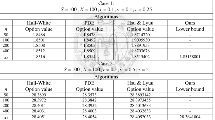
T t+ t T+ T floating dt T T Se T t t T t Se T e V 0 * 2 1 * 2 1 3 / 2 / 3 / ) 2 / )( T / ( 2 2 γ σ σ _{α σ} γ σ σ α .

Case 1: Algorithms

Hull-White PDE Hsu & Lyuu Ours

n Option value Option value Option value Lower bound

50 1.8486 1.8478 1.8714720 - 100 1.8501 1.8492 1.9095930 - 200 1.8508 1.8503 1.8891953 - 400 1.8512 1.8509 1.8703678 - ∞ 1.8516 1.8514 1.8515402 1.85158801 Case 2: 5 ; 5 . 0 ; 1 . 0 ; 100 ; 100 = = = = = X r σ τ S Algorithms

Hull-White PDE Hsu & Lyuu Ours

n Option value Option value Option value Lower bound

50 28.3899 28.3573 28.3893142 - 100 28.3972 28.3842 28.3973455 - 200 28.4011 28.3952 28.4013633 - 400 28.4031 28.4003 28.4032833 - ∞ 28.4051 28.4054 28.4052033 28.3641004 25 . 0 ; 1 . 0 ; 1 . 0 ; 100 ; 100

Chapter 4

Numerical Results

4.1 Numerical Results

= = = = = X r σ τ S

Table 1: Comparison with the Hull-White and PDE methods and Hsu and Lyuu (2005). The parameters are from Tables 3 and 4 of Forsyth et al. (2002) and Table 1 of Hsu and Lyuu (2005). The numbers quoted for the Hull-White are based on calculations using the finest grids. The “∞” row lists the extrapolated option values.

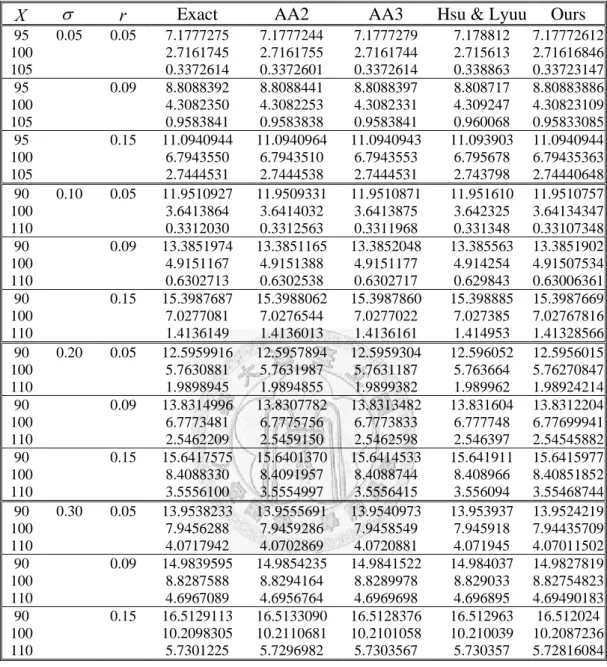
X σ r Exact AA2 AA3 Hsu & Lyuu Ours 95 0.05 0.05 7.1777275 7.1777244 7.1777279 7.178812 7.17772612 100 2.7161745 2.7161755 2.7161744 2.715613 2.71616846 105 0.3372614 0.3372601 0.3372614 0.338863 0.33723147 95 0.09 8.8088392 8.8088441 8.8088397 8.808717 8.80883886 100 4.3082350 4.3082253 4.3082331 4.309247 4.30823109 105 0.9583841 0.9583838 0.9583841 0.960068 0.95833085 95 0.15 11.0940944 11.0940964 11.0940943 11.093903 11.0940944 100 6.7943550 6.7943510 6.7943553 6.795678 6.79435363 105 2.7444531 2.7444538 2.7444531 2.743798 2.74440648 90 0.10 0.05 11.9510927 11.9509331 11.9510871 11.951610 11.9510757 100 3.6413864 3.6414032 3.6413875 3.642325 3.64134347 110 0.3312030 0.3312563 0.3311968 0.331348 0.33107348 90 0.09 13.3851974 13.3851165 13.3852048 13.385563 13.3851902 100 4.9151167 4.9151388 4.9151177 4.914254 4.91507534 110 0.6302713 0.6302538 0.6302717 0.629843 0.63006361 90 0.15 15.3987687 15.3988062 15.3987860 15.398885 15.3987669 100 7.0277081 7.0276544 7.0277022 7.027385 7.02767816 110 1.4136149 1.4136013 1.4136161 1.414953 1.41328566 90 0.20 0.05 12.5959916 12.5957894 12.5959304 12.596052 12.5956015 100 5.7630881 5.7631987 5.7631187 5.763664 5.76270847 110 1.9898945 1.9894855 1.9899382 1.989962 1.98924214 90 0.09 13.8314996 13.8307782 13.8313482 13.831604 13.8312204 100 6.7773481 6.7775756 6.7773833 6.777748 6.77699941 110 2.5462209 2.5459150 2.5462598 2.546397 2.54545882 90 0.15 15.6417575 15.6401370 15.6414533 15.641911 15.6415977 100 8.4088330 8.4091957 8.4088744 8.408966 8.40851852 110 3.5556100 3.5554997 3.5556415 3.556094 3.55468744 90 0.30 0.05 13.9538233 13.9555691 13.9540973 13.953937 13.9524219 100 7.9456288 7.9459286 7.9458549 7.945918 7.94435709 110 4.0717942 4.0702869 4.0720881 4.071945 4.07011502 90 0.09 14.9839595 14.9854235 14.9841522 14.984037 14.9827819 100 8.8287588 8.8294164 8.8289978 8.829033 8.82754823 110 4.6967089 4.6956764 4.6969698 4.696895 4.69490183 90 0.15 16.5129113 16.5133090 16.5128376 16.512963 16.512024 100 10.2098305 10.2110681 10.2101058 10.210039 10.2087236 110 5.7301225 5.7296982 5.7303567 5.730357 5.72816084

Table 2: Comparison with Zhang (2001, 2003) and Hsu and Lyuu (2005). The

parameters are from Table 1 of Zhang (2003) and Table 2 of Hsu and Lyuu (2005). The options are calls with S =100 and τ =1.

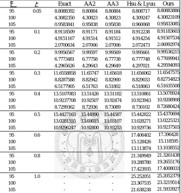
X σ Exact AA2 AA3 Hsu & Lyuu Ours 95 0.05 8.8088392 8.80884 8.80884 8.808717 8.80883886 100 4.3082350 4.30823 4.30823 4.309247 4.30823109 105 0.9583841 0.95838 0.95838 0.960068 0.95833085 95 0.1 8.9118509 8.91171 8.91184 8.912238 8.91183603 100 4.9151167 4.91514 4.91512 4.914254 4.91507534 105 2.0700634 2.07006 2.07006 2.072473 2.06992974 95 0.2 9.9956567 9.99597 9.99569 9.995661 9.99536215 100 6.7773481 6.77758 6.77738 6.777748 6.77699941 105 4.2965626 4.29643 4.29649 4.297021 4.29594093 95 0.3 11.6558858 11.65747 11.65618 11.656062 11.6547575 100 8.8287588 8.82942 8.82900 8.829033 8.82754823 105 6.5177905 6.51763 6.51802 6.518063 6.51635508 95 0.4 13.5107083 13.51426 13.51182 13.510861 13.5078924 100 10.9237708 10.92507 10.92474 10.923943 10.9208908 105 8.7299362 8.72936 8.73089 8.730102 8.72680424 95 0.5 15.4427163 15.44890 15.44587 15.442822 15.4370694 100 13.0281555 13.03015 13.03107 13.028271 13.0225321 105 10.9296247 10.92800 10.93253 10.929736 10.9237503 95 0.6 - - - 17.406402 17.396428 100 - - - 15.128426 15.118595 105 - - - 13.113874 13.1038552 95 0.8 - - - 21.349949 21.3261438 100 - - - 19.288780 19.2655176 105 - - - 17.423935 17.4008033 95 1.0 - - - 25.252051 25.2052379 100 - - - 23.367535 23.3219514 105 - - - 21.638238 21.5933927

Table 3: Comparison with Zhang (2001, 2003) and Hsu and Lyuu (2005) with a wide range of volatilities. The parameters are from Table 2 of Zhang (2003) and Table 3 of Hsu and Lyuu (2005). The options are calls with S =100, r=0.09, and τ =1.

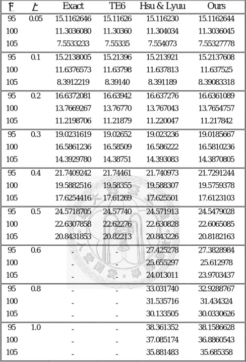
Table 4: Comparison with Ju (2002) and Zhang (2001) and Hsu and Lyuu (2005) . The exact values are based on Zhang (2001) and quoted from Table 7 of Zhang (2001). Ju's Taylor expansion method is denoted as TE6. The parameters are from Table 2 of Ju (2002) and Table 7 of Zhang (2001) and Table 4 of Hsu and Lyuu (2005). The options are calls with , , and .

X σ Exact TE6 Hsu & Lyuu Ours 95 0.05 15.1162646 15.11626 15.116230 15.1162644 100 11.3036080 11.30360 11.304034 11.3036045 105 7.5533233 7.55335 7.554073 7.55327778 95 0.1 15.2138005 15.21396 15.213921 15.2137608 100 11.6376573 11.63798 11.637813 11.637525 105 8.3912219 8.39140 8.391189 8.39083318 95 0.2 16.6372081 16.63942 16.637276 16.6361089 100 13.7669267 13.76770 13.767043 13.7654757 105 11.2198706 11.21879 11.220047 11.217842 95 0.3 19.0231619 19.02652 19.023236 19.0185667 100 16.5861236 16.58509 16.586222 16.5810236 105 14.3929780 14.38751 14.393083 14.3870805 95 0.4 21.7409242 21.74461 21.740973 21.7291244 100 19.5882516 19.58355 19.588307 19.5759378 105 17.6254416 17.61269 17.625501 17.6123103 95 0.5 24.5718705 24.57740 24.571913 24.5479028 100 22.6307858 22.62276 22.630828 22.6065085 105 20.8431853 20.82213 20.843226 20.8182163 95 0.6 _{- -} 27.425278 27.3828984 100 _{- -} 25.655297 25.612978 105 _{- -} 24.013011 23.9703437 95 0.8 _{- -} 33.031740 32.9288767 100 _{- -} 31.535716 31.434324 105 _{- -} 30.133505 30.0330626 95 1.0 _{- -} 38.361352 38.1586628 100 _{- -} 37.085174 36.8860543 105 _{- -} 35.881483 35.685358 100 = S r=0.09 τ =3

τ = 1 τ = 3

X σ Exact PDE1 PDE2 Hsu & Lyuu Ours Exact PDE1 PDE2 Hsu &

Lyuu Ours 95 0.05 8.8088392 8.8088241 8.8088241 8.808717 8.80883886 15.1162646 15.1162526 15.1162526 15.116230 15.1162644 100 4.3082350 4.3080602 4.3080602 4.309247 4.30823109 11.3036080 11.3035792 11.3035792 11.304034 11.3036045 105 0.9583841 0.9583277 0.9583277 0.960068 0.95833085 7.5533233 7.5531978 7.5531978 7.554073 7.55327778 95 0.1 8.9118509 8.9118054 8.9118054 8.912238 8.91183603 15.2138005 15.2137661 15.2137661 15.213921 15.2137608 100 4.9151167 4.9150253 4.9150253 4.914254 4.91507534 11.6376573 11.6376011 11.6376011 11.637813 11.637525 105 2.0700634 2.0700251 2.0700251 2.072473 2.06992974 8.3912219 8.3911498 8.3911498 8.391189 8.39083318 95 0.2 9.9956567 9.9956323 9.9956323 9.995661 9.99536215 16.6372081 16.6371770 16.6371770 16.637276 16.6361089 100 6.7773481 6.7773279 6.7773279 6.777748 6.77699941 13.7669267 13.7668950 13.7668950 13.767043 13.7654757 105 4.2965626 4.2964614 4.2964614 4.297021 4.29594093 11.2198706 11.2198412 11.2198412 11.220047 11.217842 95 0.3 11.6558858 11.6558892 11.6558892 11.656062 11.6547575 19.0231619 19.0230953 19.0231388 19.023236 19.0185667 100 8.8287588 8.8287699 8.8287699 8.829033 8.82754823 16.5861236 16.5860134 16.5861083 16.586222 16.5810236 105 6.5177905 6.5178134 6.5178134 6.518063 6.51635508 14.3929780 14.3927638 14.3929591 14.393083 14.3870805 95 0.4 13.5107083 13.5107373 13.5107373 13.510861 13.5078924 21.7409242 21.7359140 21.7409067 21.740973 21.7291244 100 10.9237708 10.9238047 10.9238049 10.923943 10.9208908 19.5882516 19.5801909 19.5882367 19.588307 19.5759378 105 8.7299362 8.7299785 8.7299789 8.730102 8.72680424 17.6254416 17.6129231 17.6254290 17.625501 17.6123103 95 0.5 15.4427163 15.4427436 15.4427631 15.442822 15.4370694 24.5718705 24.5164835 24.5718583 24.571913 24.5479028 100 13.0281555 13.0281668 13.0282104 13.028271 13.0225321 22.6307858 22.5534589 22.6307744 22.630828 22.6065085 105 10.9296247 10.9295940 10.9296853 10.929736 10.9237503 20.8431853 20.7378307 20.8431724 20.843226 20.8182163 95 0.6 - 17.4057119 17.4063840 17.406402 17.396428 - 27.1922830 27.4252385 27.425278 27.3828984 100 - 15.1272033 15.1284092 15.128426 15.118595 - 25.3547907 25.6552489 25.655297 25.612978 105 - 13.1117954 13.1138637 13.113874 13.1038552 - 23.6323908 24.0129680 24.013011 23.9703437 95 0.8 - 21.3206229 21.3500057 21.349949 21.3261438 - 31.8446547 33.0316957 33.031740 32.9288767 100 - 19.2465024 19.2888389 19.288780 19.2655176 - 30.1240393 31.5356736 31.535716 31.434324 105 - 17.3646285 17.4239955 17.423935 17.4008033 - 28.4742281 30.1334450 30.133505 30.0330626 95 1.0 - 25.0465250 25.2521580 25.252051 25.2052379 - 35.4451734 38.3595938 38.361352 38.1586628 100 - 23.1006194 23.3676388 23.367535 23.3219514 - 33.7509030 37.0830464 37.085174 36.8860543 105 - 21.2980435 21.6383464 21.638238 21.5933927 - 32.1020703 35.8789184 35.881483 35.685358

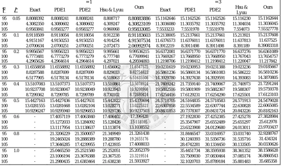
Table 5: Comparison with the one-dimensional PDE method of Ve ~c~er (2001) and Hsu and Lyuu (2005).PDE1 is based on the 2000

100× grid over

[ ] [

0,τ × −1,1

]

.PDE2 is based on the100×10000grid over

[ ] [

0,τ × −1,9

]

. The parameters and numerical data for Exact and Hsu & Lyuu are from Tables 3 and 4. The numerical data for PDE1 and PDE2 are from Hsu (2005).The options are calls with S =100 and r=0.09.

X σ Lower Bound Hsu & Lyuu Fusai Exact Monte Carlo Ours 95 0.05 8.8088 8.808717 8.80885 8.8088392 8.81 8.80883886 100 4.3082 4.309246 4.30824 4.3082350 4.31 4.30823109 105 0.9583 0.960069 0.95839 0.9583841 0.95 0.95833085 95 0.10 8.9118 8.912238 8.91185 8.9118509 8.91 8.91183603 100 4.9150 4.914254 4.91512 4.9151167 4.91 4.91507534 105 2.0699 2.072473 2.07007 2.0700634 2.06 2.06992974 90 0.30 14.9827 14.984037 14.98396 - 14.96 14.9827819 100 8.8275 8.829033 8.82876 8.8287588 8.81 8.82754823 110 4.6949 4.696895 4.69671 - 4.68 4.69490183 90 0.50 18.1829 18.188933 18.18885 - 18.14 18.1829569 100 13.0225 13.028271 13.02816 13.0281555 12.98 13.0225321 110 9.1179 9.124414 9.12432 - 9.10 9.11794987 90 0.60 - 19.964542 - - 19.94 19.9541628 100 - 15.128426 - - 15.13 15.118595 110 - 11.342769 - - 11.36 11.3322821 90 0.80 - 23.622784 - - 23.61 23.5980253 100 - 19.288780 - - 19.33 19.2655176 110 - 15.739790 - - 15.74 15.7164077 90 1.00 - 27.305012 - - 27.25 27.256476 100 - 23.367535 - - 23.36 23.3219514 110 - 20.051542 - - 20.03 20.0069488

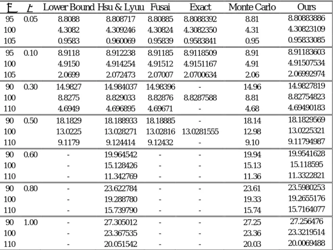
Table 6: Comparison with the lower bounds of Rogers and Shi (1995) and Hsu and Lyuu (2005). The parameters, lower bounds, and Monte Carlo results for

are from Table 3 of Rogers and Shi (1995) and Table 1 of Thompson (1999). The Monte Carlo results for are based on simulation paths. The options are calls with , , and . Hsu & Lyuu algorithm's computed option values and the exact option values are from Table 3. Fusai is based on the data in Table 3 of Fusai (2004) computed using the most computing times. The two boxed numbers are lower than the lower bounds of Rogers and Shi.

5 . 0 ≤ σ 5 . 0 ≥ σ 6 10 2× 100 = S r=0.09 τ =1 21

X σ Lower Bound Hsu & Lyuu Hsu & Lyuu

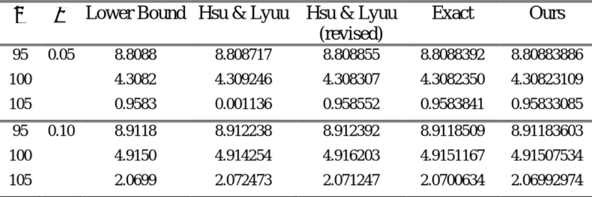
(revised) Exact Ours 95 0.05 8.8088 8.808717 8.808855 8.8088392 8.80883886 100 4.3082 4.309246 4.308307 4.3082350 4.30823109 105 0.9583 0.001136 0.958552 0.9583841 0.95833085 95 0.10 8.9118 8.912238 8.912392 8.9118509 8.91183603 100 4.9150 4.914254 4.916203 4.9151167 4.91507534 105 2.0699 2.072473 2.071247 2.0700634 2.06992974

Table 7: Comparison with the lower bounds of Rogers and Shi (1995) and Hsu and Lyuu (2005) using the revised algorithm. The data and parameters are from Table 6 except that the revised algorithm incorporates tighter running-sum ranges.

Sigma σ Interest Rate r Roger & Shi Lower Ours 0.1 0.05 1.2454 1.24541 0.09 0.6992 0.699247 0.15 0.2516 0.251641 0.2 0.05 3.4044 3.40441 0.09 2.6216 2.62164 0.15 1.7098 1.70982 0.3 0.05 5.6246 5.62469 0.09 4.7382 4.73822 0.15 3.6085 3.60852

Table 8: Comparison with the lower bounds of Rogers and Shi (1995) on foating-strike Asian option prices for S =100 with an expiry time of 1 year.

Chapter 5

Conclusions and Future Work

We extend Thompson (1998) a lower bound to price fixed-strike and floating-strike Asian options. The results can be summarized as follows:

y When volatility is small, the result of our approximation approaches the exact result with the difference starting from ten-thousandths place.

A′ A′

y When volatility is large, the result of our approximation approaches the exact result with the difference starting from one-hundredth place.

y We can get lower bounds efficiently.

y As stated above, our lower bound deteriorates somewhat when the volatility is large. A better approximate lower bound may be possible by replacing

approximation A′ with a different one. That may be a course for future work . y If stock price does not follow a generalized Browning motion, we cannot use this

approximation formula. We should try to seek for another approximation formula under this situation.

Appendix

In this appendix, we will prove two theorems.

Proof for Theorem 2.5 Two random variable with and

then _⎟⎟ ⎠ y ⎞ ⎜ ⎜ ⎝ ⎛ + Φ = > u + y X_{I Y e} c e E x x σ µ σ2 2 1

0 where Φ

( )

⋅ is the normal

distribution function ,I(⋅) is the indicator function and c=Cov

(

X ,Y

)

. Y X ,

(

2

)

, ~ _{x x} X φ µ σ

(

2

)

, ~ _{y y} Y φ µ σ

(

(

)

)

Proof: By definition of Expectation,

(

)

(

e I Y

)

e e ( ) dydx. E y y y y x x x x x y y x y x x X

∫ ∫

−∞∞ ∞ _⎪⎭ ⎪ ⎬ ⎫ ⎪⎩ ⎪ ⎨ ⎧ ⎟ ⎟ ⎠ ⎞ ⎜ ⎜ ⎝ ⎛ − + ⎟ ⎟ ⎠ ⎞ ⎜ ⎜ ⎝ ⎛ − ⎟⎟ ⎠ ⎞ ⎜⎜ ⎝ ⎛ − ⎟⎟ ⎠ ⎞ ⎜⎜ ⎝ ⎛ − − − − = > 0 2 -1 2 1 2 2 2 2 1 2 0 σ µ σ µ σ µ ρ σ µ ρ ρ σ πσ

Let Then , and we can get

( ){u2 ρuv+v2}_dvdu 2 -2 y y x x _v y x u σ µ σ µ − = − = . , dxdy=σ_xσ_ydudv e e y y x x u

∫ ∫

−∞∞ ∞ − − − + _⋅ − = σ µ σ µ ρ ρ π 1 2 1 2 1 2 1 ( )

{

( ) ( )

}

_dvdu e e e y y x x u v v u

∫ ∫

−∞∞ ∞ − + − − ⋅ − = σ µ ρ ρ ρ σ µ ρ π 2 2 2 2 1 -1 2 1 2 1 2 ( ) ( ) _dvdu e e e y y x x u v v u

∫ ∫

−∞∞ ∞ − − + − − ⋅ − = σ µ ρ ρ σ µ ρ π 2 -1 2 2 2 2 2 1 2 . 2 1 ρ ρ − − = u v w 25

We change the variables again: . Then ,and we get

dwdv x v v _{+σ ρ⋅} 2 2 2 1−ρ = du dw e e e y y x x w _w

∫

−∞

∫

∞ ∞ − − ⋅ − + − ⋅ = σ µ ρ σ µ π 1 2 2 2 2

( ) dw e dv e e y y x x x x _v w

∫

−∞

∫

∞ ∞ − ⎟ ⎠ ⎞ ⎜ ⎝ ⎛ _{− −} − − − ⋅ + ⋅ = σ µ ρ σ ρ σ σ µ π π 2 1 2 1 5 . 0 2 2 2 2 2 1 2

( )

2 1 2 2 2 1 ⎟⎠ ⎞ ⎜ ⎝ ⎛ _{− −} − = ρ σ π x w e w f

Given that is a PDF, then , and

the above equals

( ) ∞ − v−σxρ2 1 1 2 1 ₂ 1 2 2 =

∫

−∞∞ ⎟ ⎠ ⎞ ⎜ ⎝ ⎛ _{− −} − dw e x wσ ρ π

∫

− ⋅ + = y y x x dv e e σ µ σ µ π 2 2 5 . 0 2 k = −

We can change variables: . Then ,we can reduce above equation

dk 2 dv dk = ρ σ_x v e e dk e e x y y x x x y y x x _{k k}

∫

∫

−∞+ − ⋅ + ∞ − − − ⋅ + = = σ σ ρ µ σ µ ρ σ σ µ σ µ π π 1 5 . 0 2 1 5 . 0 2 2 2 2 2 2 ⎞ ⎛ + ⎞ ⎛µ µ c

(by the symmetry property of normal distribution)

⎟ ⎟ ⎠ ⎜ ⎜ ⎝ Φ × = ⎟ ⎟ ⎠ ⎜ ⎜ ⎝ + Φ × = + ⋅ + ⋅ y y x y y e e x x x x σ ρ σ σ σ µ σ µ _0.5 2 _0.5 2 .

Proof for Theorem 2.6

For any random variable X with density , we have

1

( )

x f_X

(

) (

)

[

] [

]

(i) S E T dt X K S E T

∫

t − > =

∫

∂ 0 0 γ γ = − > > −K I X E S K X S E _{t t} ; (ii) 26

(

)

T

(

_t K X

)

(

f_X

( )

x

)

dt T − = − ∂ | ; 1 _{γ γ} λ

(

) (

)

[

]

_{∫ ∫}

∞

(

) (

)

(

)

∞ − ∞ ∞ − − > = > − _{t B X t t} t K I X S K I X f B X dXdB S t , , γ γ ∞ ∞ Proof: (i)

(

−

)

(

)

=

[

− >γ

]

=

_{∫ ∫}

∞ − r St K fBt ,X Bt ,X dXdBt E St K;X

(ii) By the definition of expectation,

.

(

)

(

)

T 1 ∞ ∂ ∞

(

)

(

S K

)

f

(

B X

)

dXdBdt T dt X K S E T B X t t T t T t t , 1 ; 1 , 0 0

∫ ∫ ∫

∫

−∞∞ ∞ − ∂ ∂ = > − ∂ ∂ γ γ γ λ

We can exchange the integral and the partial derivative to get

(

S K

)

f

(

B X

)

dXdBdt T B X t t T t t , 1 , 0

∫ ∫

−∞∞

∫

∞ − ∂ ∂ = γ γ dt dXdB X B f K S T

∫ ∫

_{0 −∞}∂

∫

t − Bt,X t , t = γ γ .

(

)

(

)

T ∞ 1 By Leibnitz’s Rule,

(

)

(

)

( )

_{( )}

dB_tdt f f B f K S T _X X T t X B t t γ γ γ ⋅ − − =

∫ ∫

∞ ∞ − 0 , , 1 dt dB B f K S T

∫ ∫

_−∞− t − Bt X t t = 0 , ,γ

(

S K

)

f

(

B

) ( )

f dBdt T X t T t X B t − t γ ⋅ γ − =

_{∫ ∫}

∞ ∞ − 0 , | 1 . 1 T

By the definition of expectation, the above equals

(

)

(

( )

)

0 E St K X| fX x dt

T

∫

− =γ − .

Bibliography

[1] Yuh-Dauh Lyuu, Financial Engineering and Computation. Cambridge University Press, UK, 2002.

[2] Paul G. Hoel, Sidney C. Port, and Charles J. Stone, Introduction to Stochastic Processes. Waveland Press , NJ, 1986.

[3] John C. Hull, Options, Futures, and Other Derivatives. 5th Edtion, Prentice Hall, Englewood Cliffs, NJ, 2003.

[4] Tomas Bjork, Arbitrage Theory in Continuous Time. Oxford University Press, NY, 1998.

[5] J . Michael Steele, Stochastic Calculus and Financial Applications. Springer, NY, 2001.

[6] Sheldon Ross, A First Course in Probability. 5th Edtion, Prentice Hall, NJ, 1998.

[7] J. Aase Nielsen and Klaus Sandmann. “Pricing Bounds on Asian Options.” Journal of Financial and Quantitative Analysis, 38, No. 2 (June 2003), 449–473.

[8] Vicky Henderson and Rafal Wojakowski. “On the Equivalence of Floating- and Fixed-Strike Asian Options.” Journal of Applied Probability, 39(2), 2002, 391–394.