IEEE 802.16e OFDMA 下行同步技術之探討與數位訊號處理器實現

國

立

交

通

大

學

電子工程學系 電子研究所碩士班

碩

士

論

文

IEEE 802.16e OFDMA 下行同步技術之探討與數位

訊號處理器實現

Research in and DSP Implementation of

Synchronization Techniques for IEEE 802.16e

OFDMA Downlink

研 究 生：洪 潤 傑

指導教授：桑 梓 賢 教授

IEEE 802.16e OFDMA 下行同步技術之探討與數位訊號處理器

實現

Research in and DSP Implementation of Synchronization

Techniques for IEEE 802.16e OFDMA Downlink

研 究 生：洪潤傑 Student：Jun-Chieh Hung

指導教授：桑梓賢 教授 Advisor：Tzu-Hsien Sang

國 立 交 通 大 學

電子工程學系 電子研究所碩士班

碩 士 論 文

Submitted to College of Electrical and Computer Engineering National Chiao Tung University

in Partial Fulfillment of the Requirements for the Degree of

Master in

Electronics Engineering January 2008

Hsinchu, Taiwan, Republic of China

IEEE 802.16e OFDMA 下行同步技術之探討與數位訊號

處理器實現

研究生：洪潤傑 指導教授：桑梓賢 教授

國立交通大學

電子工程研究所碩士班

摘要

本篇論文提出IEEE 802.16e 正交分頻多工存取(OFDMA)下行(downlink)過程

中起始同步的機制，包含符碼時間偏移、載波偏移的同步與基地台(cell)同步碼索 引(preamble index)的識別。當一個行動電話在一開始要進入網路的時候，我們必 須做起始的同步。我們提出的方法不需要傳送端同步碼的訊息，只需利用同步碼 的結構、循環字首(cyclic prefix)以及傅立葉轉換(Fourier transform)的性質，即可做 到時間和頻率的同步，與基地台同步碼索引的識別。而在之後的次訊框裡，行動 電話只需要做到追蹤符碼時間偏移和小數部分載波偏移即可。 我們首先用浮點數運算來驗證起始同步的技術，並在多路徑 Rayleigh 衰減 通道下做模擬，模擬速度大約120 km/h，並觀察其結果。最後，我們選擇最適合 我們系統的同步演算法，並把這些方法修改成定點運算的版本，實現在數位訊號 處理(DSP)平台上。

Research in and DSP Implementation of Synchronization

Techniques for IEEE 802.16e Downlink

Student：Jun-Chieh Hung Advisor：Tzu-Hsien Sang

Department of Electronics Engineering & Institute of Electronics

National Chiao Tung University

ABSTRACT

In this thesis, we propose an initial synchronization scheme for time, carrier frequency synchronization and cell preamble index identification in 802.16e OFDMA downlink. In DL synchronization, the mobile station receiver needs to perform initial synchronization upon its initial entrance to the network. The proposed method does not require knowledge of actual transmitted preamble, but only utilizes the preamble structure, CP, and inverse Fourier transform properties to obtain time/frequency synchronization and cell preamble index identification. Then in subsequent sub-frame, the mobile station only needs to track the timing and fractional CFO.

We verify the initial synchronization techniques in floating point computation, simulate in multi-path Rayleigh fading channel which the speed is about 120 km/h, and see the performance. In the end, we choose the most suitable methods for our system into fixed point version on the DSP platform.

誌 謝

另外也感謝S&C 實驗室(S&C Lab)提供了舒適的研究環境與充足的軟硬體設

備以及資策會(III)的慷慨支援，讓我在研究中不虞匱乏，能夠專心投入。

最後，感謝我的父母，無怨無悔的給予我生活上與精神上的支持，以及身邊 的朋友在我苦惱的時候鼓勵我，陪我走過這最後的求學時光，感謝各位。

Contents

Chapter 1 Overview of Physical Layer (PHY) IEEE 802.16e OFDMA ... 1

1.1 Introduction to OFDM and OFDMA Systems ... 1

1.2 Introduction to Mobile WiMAX ... 3

1.3 Introduction to IEEE 802.16e Downlink... 4

1.3.1 OFDMA Frame Structure ... 4

1.3.2 OFDMA Symbol Structure... 5

Chapter 2 Synchronization Techniques for IEEE 802.16e Downlink ... 8

2.1 Channel Model and System Parameters ... 8

2.1.1 Modified Stanford University Interim (SUI) Channel Models . 8 2.1.2 System Parameters...11

2.2 Synchronization Control Mechanisms ... 13

2.2.1 Network Synchronization ... 13

2.2.2 SS Synchronization ... 13

2.2.3 Frequency Control Requirements ... 14

2.3 Mobile Station Synchronization Techniques... 15

2.3.1 Symbol Timing Estimation... 16

2.3.2 Fractional CFO Estimation... 25

Chapter 3 DSP Implementation of IEEE 802.16e Downlink System ... 36

3.1 Introduction to the DSP Platform... 36

3.1.1 MSC8126ADS Board Architecture... 36

3.1.2 MSC8126 Features ... 38

3.1.3 Developing Optimized Code for Speed on SC140 Cores ... 41

3.2 Implementation of Transmitter... 43

3.3 Performance Analysis of Synchronization Implementation... 50

3.3.1 Symbol Timing Estimation... 50

3.3.2 Fractional CFO Estimation... 52

3.3.3 Summary of Implementation Analysis for Synchronization ... 54

3.3.4 Integer CFO Estimation and Preamble Index Identification.. 58

3.4 WiMAX System Integration on the DSP Platform ... 60

Chapter 4 Conclusions and Future Work ... 62

4.1 Conclusions ... 62

4.2 Future Work ... 63 Bibliography 64

List of Figures

Fig. 1.1 Basic architecture of an OFDM system. (Source: [3]) ... 2

Fig. 1.2 OFDMA sub-carriers. ... 2

Fig. 1.3 Mobile WiMAX system profile. (Source: [3]) ... 3

Fig. 1.4 Example of an OFDMA frame (with only mandatory zone) in TDD mode. (Source: [5]) ... 5

Fig. 1.5 Cluster structure. (Source: [3])... 7

Fig. 2.1 Structure of initial DL synchronization. (Source: [7])... 16

Fig. 2.2 Preamble and CP delay correlation under SUI-3 channel... 19

Fig. 2.3 Symbol time synchronization error distribution under SUI-3 channel with 0 Hz, 150 Hz, and 300 Hz Doppler frequency using different methods.23 Fig. 2.4 RMSE of symbol timing offset synchronization using different methods under SUI-3 channel with 0 Hz, 150 Hz, and 300 Hz Doppler frequency... 25

Fig. 2.5 Fractional CFO synchronization error distribution under SUI-3 channel with 0 Hz, 150 Hz, and 300 Hz Doppler frequency. ... 29

Fig. 2.6 RMSE of fractional CFO synchronization under SUI-3 channel with 0 Hz, 150 Hz, and 300 Hz Doppler frequency... 30

Fig. 2.7 The sub-carrier permutation of different segments near the guard band. ... 32 Fig. 2.8 Error probability of preamble index identification after coarse integer

and search range. ... 33

Fig. 2.9 Error probability of either the estimated integer CFO or the identified preamble index under SUI-3 channel with different methods. ... 34

Fig. 3.1 MSC8122/8126ADS top-side part location diagram. (Source: [10]) 37 Fig. 3.2 MSC8126 block diagram. (Source: [11])... 39

Fig. 3.3 SC140 extended core block diagram. (Source: [11])... 40

Fig. 3.4 WiMAX PHY interfaces. ... 43

Fig. 3.5 DL UP chain on MSC8126. ... 44

Fig. 3.6 DL FP processing functions. ... 45

Fig. 3.7 DL carrier scrambling scheme. ... 46

Fig. 3.8 Histogram of UP function cycle count... 48

Fig. 3.9 Histogram of FP function cycle count. ... 49

Fig. 3.10 RMSE of symbol timing offset synchronization under SUI-3 channel.52 Fig. 3.11 RMSE of fractional CFO synchronization under SUI-3 channel with 0 Hz, 150 Hz, and 300 Hz Doppler frequency comparing with fixed point and floating point... 53

Fig. 3.12 Histogram of initial synchronization function cycle count (using preamble). ... 55 Fig. 3.13 Histogram of initial synchronization function cycle count (using

CP). 56

Fig. 3.14 Fixed point implementation results of symbol timing estimation using different correlation under SUI-3 channel with 0 Hz, 150 Hz, and 300 Hz

Doppler frequency. ... 58 Fig. 3.15 Error probability of either the estimated integer CFO or the identified

preamble index under SUI-3 channel with 0 Hz, 150 Hz, and 300 Hz

List of Tables

Table 2.1 Terrain Type vs. SUI Channels ... 9

Table 2.2 General Characteristic of SUI Channels... 9

Table 2.3 SUI-1 Channel Model ... 9

Table 2.4 SUI-2 Channel Model ... 10

Table 2.5 SUI-3 Channel Model ... 10

Table 2.6 SUI-4 Channel Model ... 10

Table 2.7 SUI-5 Channel Model ... 10

Table 2.8 SUI-6 Channel Model ... 10

Table 2.9 OFDMA Scalability Parameters ... 12

Table 3.1 MSC8126ADS Board Features ... 38

Table 3.2 MSC8126 Features ... 41

Table 3.3 Cycle Count of DL UP ... 48

Table 3.4 Cycle Count of DL FP ... 49

Table 3.5 Cycle Count of Initial Synchronization using Preamble ... 55

Table 3.6 Cycle Count of Initial Synchronization using CP ... 56

Table 3.7 Cycle Count of Integer CFO Search for Different Methods per One Preamble Index... 60

Table 3.8 Throughput of WiMAX 16e Transmitter on MSC8126... 61

Chapter 1

Overview of Physical Layer (PHY)

IEEE 802.16e OFDMA

1.1 Introduction to OFDM and OFDMA Systems

Orthogonal frequency division multiplexing (OFDM) in [1] and [2] is a multiplexing technique that subdivides the bandwidth into multiple frequency sub-carriers as shown in Fig. 1.1. In an OFDM system, the input data stream is divided into several parallel sub-streams of reduced data rate (thus increased symbol duration) and each sub-stream is modulated and transmitted on a separate orthogonal sub-carrier. The increased symbol duration improves the robustness of OFDM to channel delay spread. The sub-carriers have the minimum frequency separation required to maintain orthogonality of their corresponding time domain waveforms, yet the signal spectra corresponding to the different sub-carriers overlap in frequency. Hence, the available bandwidth is used very efficiently. Furthermore, the introduction of the cyclic prefix (CP) can completely eliminate inter-symbol interference (ISI) as long as the CP duration is longer than the channel delay spread. OFDM modulation can be realized with efficient IFFT, which enables a large number of sub-carriers (up to 2048) with low complexity.

Fig. 1.1 Basic architecture of an OFDM system. (Source: [3])

Orthogonal frequency division multiple access (OFDMA) in [4] and [5] is a multiple-access/multiplexing scheme that provides multiplexing operation of data streams from multiple users onto the downlink sub-channels and uplink multiple access is achieved by assigning subsets of sub-carriers to individual users as shown in Fig. 1.2. This allows simultaneous low data rate transmission from several users. Different number of sub-carriers can be assigned to different users, in view to support differentiated quality of service (QoS), i.e. to control the data rate and error probability individually for each user.

1.2 Introduction to Mobile WiMAX

The WiMAX technology, based on the IEEE 802.16-2004 air interface standard [4] is rapidly proving itself as a technology that will play a key role in fixed broadband wireless metropolitan area networks. Mobile WiMAX that adopts OFDMA for improved multi-path performance in non-line-of-sight environments is a broadband wireless solution that enables convergence of mobile and fixed broadband networks through a common wide area broadband radio access technology and flexible network architecture. It offer scalability in both radio access technology and network architecture, thus providing a great deal of flexibility in network deployment options and service offerings. Scalable OFDMA (SOFDMA) is introduced in the IEEE 802.16e standard [5] amendment to support scalable channel bandwidths from 1.25 to 20 MHz. Release-1 mobile WiMAX profiles that is completed in early 2006 (see Fig. 1.3 from [3]) will cover 5, 7, 8.75, and 10 MHz channel bandwidths for licensed worldwide spectrum allocations in the 2.3 GHz, 2.5 GHz, 3.3 GHz and 3.5 GHz frequency bands.

1.3 Introduction to IEEE 802.16e Downlink

In OFDMA, the active sub-carriers are divided into subsets of sub-carriers where each subset is termed a sub-channel. The sub-carriers forming one sub-channel may, but need not be, adjacent. Three basic types sub-channel organization are defined in [4] and [5]: partial usage of sub-channels (PUSC), full usage of sub-channels (FUSC), and adaptive modulation and coding (AMC) among which the PUSC is mandatory and the other two are optional. In PUSC DL, the entire channel bandwidth is divided into three segments to be used separately. The FUSC is employed only in the DL and it uses the full set of available sub-carriers so as to maximize the throughput.

1.3.1 OFDMA Frame Structure

In licensed bands, the duplexing method shall be either frequency division duplex (FDD) or time division duplex (TDD). The 802.16e PHY in [4] and [5] supports TDD and full and half-duplex FDD operation however the initial release of mobile WiMAX certification profiles will only include TDD.

Fig. 1.4 from [5] illustrates the OFDMA frame structure for a TDD implementation. Each frame is divided into DL and UL sub-frames separated by transmit/receive transition gap (TTG) and receive/transmit transition gap (RTG) to prevent DL and UL transmission collisions. In a frame, the following control information is used to ensure optimal system operation:

z Preamble: The preamble, used for synchronization, is the first OFDM symbol of the frame.

the frame configuration information such as mapping (MAP) message length and coding scheme and usable sub-channels.

z DL-MAP and UL-MAP: The DL-MAP and UL-MAP provide sub-channel allocation and other control information for the DL and UL sub-frames respectively.

z UL Ranging: The UL ranging sub-channel is allocated for mobile station (MS) to perform closed-loop time, frequency, and power adjustment as well as bandwidth requests.

Fig. 1.4 Example of an OFDMA frame (with only mandatory zone) in TDD mode. (Source: [5])

1.3.2 OFDMA Symbol Structure

As mentioned in [4] and [5], the OFDMA PHY defines four scalable FFT sizes: 2048, 1024, 512, and 128. Here we only take the 2048-FFT OFDMA sub-carrier

allocation for introduction. The sub-carriers are divided into three types: null (guard band and DC), pilot, and data. Subtracting the guard tones from scalable FFT size NFFT,

one obtains the set of “used” sub-carriers Nused. These used sub-carriers are allocated to pilot sub-carriers and data sub-carriers.

z Preamble

The first symbol of the downlink transmission is the preamble. There are three types of preamble carrier-sets, those are defined by allocation of different sub-carriers for each one of them; those sub-carriers are modulated using a boosted BPSK modulation with a specific pseudo-noise (PN) code defined in Table 309 if [4]. The preamble carrier-sets are defined using

3

n

PreambleCarrierSet = + ⋅n k (1.1)

where:

PreambleCarrierSetn specifies all sub-carriers allocated to the specific preamble,

n is the number of the preamble carrier-set indexed 0...2, k is a running index 0...567.

Each segment uses a preamble composed of a carrier-set and modulates each third sub-carrier. Because the DC carrier will not be modulated at all, it shall always be zeroed and the appropriate PN will be discarded. For the preamble symbol there will be 172 guard band sub-carriers on the left side and the right side of the spectrum. z Symbol Structure for PUSC

The symbol structure is constructed using pilots, data, and zero sub-carriers. Active (data and pilot) sub-carriers are grouped into subsets of sub-carriers called sub-channels. The minimum frequency-time resource unit of sub-channelization is one slot, which is equal to 48 data tones (sub-carriers).

With DL-PUSC, for each pair of OFDMA symbols, the available or usable sub-carriers are grouped into clusters containing 14 contiguous sub-carriers per symbol

period, with pilot and data allocations in each cluster in the even and odd symbols as shown in Fig 1.5. A re-arranging scheme is used to form groups of clusters such that each group is made up of clusters that are distributed throughout the sub-carrier space. A slot contains two clusters and is made up of 48 data sub-carriers and eight pilot sub-carriers. The data sub-carriers in each group are further permutated to generate sub-channels within the group. Therefore, only the pilot positions in the cluster are shown in Fig 1.5. The data sub-carriers in the cluster are distributed to multiple sub-channels.

Chapter 2

Synchronization Techniques for

IEEE 802.16e Downlink

2.1 Channel Model and System Parameters

2.1.1 Modified Stanford University Interim (SUI)

Channel Models

Channel models described in [6] provide the basis for specifying channels for a given scenario. It is obvious that there are many possible combinations of parameters to obtain such channel descriptions. A set of 6 typical channels was selected for the three terrain types that are typical of the continental United States. In this section we present SUI channel models that we modified to account for 30o directional antennas. These models can be used for simulations, design, development, and testing of technologies suitable for broadband wireless applications. The parametric view of the SUI channels is summarized in Table 2.1 and Table 2.2.

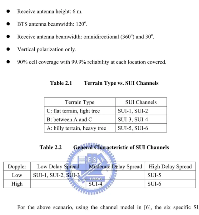
Six SUI channels are constructed which are representative of the real channels, using the general structure of the SUI Channel and assuming the following scenario: z Cell size: 7 km.

z Receive antenna height: 6 m. z BTS antenna beamwidth: 120o_.

z Receive antenna beamwidth: omnidirectional (360o) and 30o. z Vertical polarization only.

z 90% cell coverage with 99.9% reliability at each location covered.

Table 2.1 Terrain Type vs. SUI Channels

Terrain Type SUI Channels

C: flat terrain, light tree SUI-1, SUI-2

B: between A and C SUI-3, SUI-4

A: hilly terrain, heavy tree SUI-5, SUI-6

Table 2.2 General Characteristic of SUI Channels

Doppler Low Delay Spread Moderate Delay Spread High Delay Spread

Low SUI-1, SUI-2, SUI-3 SUI-5

High SUI-4 SUI-6

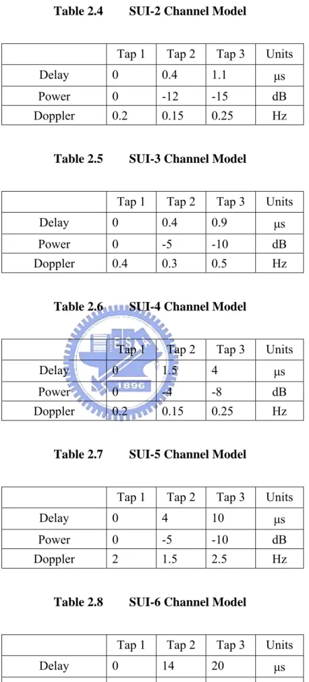
For the above scenario, using the channel model in [6], the six specific SUI channel models are list in Tables 2.3 to 2.8 and we choose SUI-3 channel model as our simulation environment.

Table 2.3 SUI-1 Channel Model

Tap 1 Tap 2 Tap 3 Units

Delay 0 0.4 0.9 μs

Power 0 -15 -20 dB

Table 2.4 SUI-2 Channel Model

Tap 1 Tap 2 Tap 3 Units

Delay 0 0.4 1.1 μs

Power 0 -12 -15 dB

Doppler 0.2 0.15 0.25 Hz

Table 2.5 SUI-3 Channel Model

Tap 1 Tap 2 Tap 3 Units

Delay 0 0.4 0.9 μs

Power 0 -5 -10 dB

Doppler 0.4 0.3 0.5 Hz

Table 2.6 SUI-4 Channel Model

Tap 1 Tap 2 Tap 3 Units

Delay 0 1.5 4 μs

Power 0 -4 -8 dB

Doppler 0.2 0.15 0.25 Hz

Table 2.7 SUI-5 Channel Model

Tap 1 Tap 2 Tap 3 Units

Delay 0 4 10 μs

Power 0 -5 -10 dB Doppler 2 1.5 2.5 Hz

Table 2.8 SUI-6 Channel Model

Tap 1 Tap 2 Tap 3 Units

Delay 0 14 20 μs

Power 0 -10 -14 dB

2.1.2 System Parameters

z Primitive Parameters

The following four primitive parameters defined in [4] characterize the OFDMA symbol:

1) BW: This is the nominal channel bandwidth.

2) Nused: Number of used sub-carriers (which includes the DC sub-carrier).

3) n: Sampling factor. This parameter, in conjunction with BW and Nused

determines the sub-carrier spacing, and the useful symbol time. This value is set as follows: for channel bandwidths that are a multiple of 1.75 MHz then n = 8/7 else for channel bandwidths that are a multiple of any of 1.25, 1.5, 2 or 2.75 MHz then n = 28/25 else for channel bandwidths not otherwise specified then n = 8/7.

4) G: This is the ratio of CP time to “useful” time. The following values shall be supported: 1/32, 1/16, 1/8, and 1/4.

z Derived Parameters

The following parameters are defined in terms of the primitive parameters: 1) NFFT: Smallest power of two greater than Nused

2) Sampling frequency:F_s =⎢_⎣n BW⋅ / 8000⎥_⎦×8000 3) Sub-carrier spacing:Δ =f Fs/NFFT

4) Useful symbol time:T_b = Δ 1/ f

5) CP time:T_g = ⋅G T_b

6) OFDMA symbol time:T_s =T_b+T_g

z Scalable OFDMA

The IEEE 802.16e OFDMA mode is based on the concept of SOFDMA. SOFDMA supports a wide range of bandwidths to flexibly address the need for various spectrum allocation and usage model requirements. The scalability is supported by adjusting the FFT size while fixing the sub-carrier frequency spacing at 10.94 kHz. Since the resource unit sub-carrier bandwidth and symbol duration is fixed, the impact to higher layers is minimal when scaling the bandwidth. The SOFDMA parameters are listed in Table 2.9 from [5]. For convenience, we only take the 512 FFT size following the parameters in Table 2.9 and QPSK data modulation to simulate and implement our OFDMA PHY downlink receiver.

Table 2.9 OFDMA Scalability Parameters

Parameters Values

System Channel Bandwidth (MHz) 1.25 5 10 20

Sampling Frequency (Fs in MHz) 1.4 5.6 11.2 22.4

FFT Size (NFFT) 128 512 1024 2048

Number of Sub-channels 2 8 16 32

Sub-carrier Frequency Spacing 10.94 kHz

Useful Symbol Time (Tb = 1/f) 91.4 microseconds

Guard Time (Tg = Tb/8) 11.4 microseconds

2.2 Synchronization Control Mechanisms

2.2.1 Network Synchronization

For TDD and FDD realizations, it is recommended (but not required) that all BSs be time synchronized to a common timing signal. In the event of the loss of the network timing signal, BSs shall continue to operate and shall automatically resynchronize to the network timing signal when it is recovered. The synchronizing reference shall be a 1 pps timing pulse and a 10 MHz frequency reference. These signals are typically provided by a global positioning system (GPS) receiver.

For both FDD and TDD realizations, frequency references derived from the timing reference may be used to control the frequency accuracy of BSs provided that they meet the frequency accuracy requirements of 2.2.3. This applies during normal operation and during loss of timing reference.

2.2.2 SS Synchronization

For any duplexing, all SSs shall acquire and adjust their timing such that all uplink OFDMA symbols arrive time coincident at the BS to an accuracy of ± 25% of the minimum guard interval or better. Ranging for time (coarse synchronization) and power is performed during two phases of operation: during (re)registration and when synchronization is lost; and second, during FDD or TDD transmission on a periodic basis.

and if successful, is entered into a ranging process under control of the BS. The ranging process is cyclic in nature where default time and power parameters are used to initiate the process followed by cycles where (re)calculated parameters are used in succession until parameters meet acceptance criteria for the new subscriber. These parameters are monitored, measured, and stored at the BS, and transmitted to the subscriber unit for use during normal exchange of data. During normal exchange of data, the stored parameters are updated in a periodic manner based on configurable update intervals to ensure changes in the channel can be accommodated. The update intervals shall vary in a controlled manner on a subscriber unit by subscriber unit basis.

Ranging on re-registration follows the same process as new registration.

2.2.3 Frequency Control Requirements

At the BS, the transmitted center frequency, receive center frequency, and the symbol clock frequency shall be derived from the same reference oscillator. At the BS, the reference frequency accuracy limited in [3] shall be better than ±2×10–6.

At the SS, both the transmitted center frequency and the sampling frequency shall be derived from the same reference oscillator. Following [4], the SS uplink transmission shall be locked to the BS, so that its center frequency shall deviate no more than 2% of the sub-carrier spacing, compared to the BS center frequency.

During the synchronization period, the SS shall acquire frequency synchronization within the specified tolerance before attempting any uplink transmission. During normal operation, the SS shall track the frequency changes by estimating the downlink frequency offset and shall defer any transmission if synchronization is lost. To determine the transmit frequency, the SS shall accumulate

the frequency offset corrections transmitted by the BS (for example in ranging response (RNG-RSP) message), and may add to the accumulated offset, an estimated UL frequency offset based on the downlink signal.

2.3 Mobile Station Synchronization Techniques

Synchronization is an essential task for any digital communication system. Without accurate synchronization algorithms, it is not possible to reliably receive the transmitted data. In OFDM system, the received signal detection requires sub-carrier orthogonality. Variations of the carrier oscillator, sampling clock or the symbol time offset affect this orthogonality. Therefore, the synchronizer estimates and compensates any offsets in carrier, sampling time, and OFDM symbol time in the receiver in reference to the transmitter.

WLAN systems typically include a preamble in the start of the packet with reference to [1]. The length and the contents of the preamble have been carefully designed to provide enough information for good synchronization performance without any unnecessary overhead.

In this chapter, we present a novel initial synchronization algorithm for downlink of OFDMA TDD based mobile WiMAX. When the MS receiver enters the network for the first time, initial DL synchronization including timing and carrier recovery will be done. We assume that the frame synchronization is done by monitoring the power of the received signal. Upon entering the network and upon a need to handover, the MS has to identify the preamble index of the BS segment that it will communicate with. Therefore, another important task needed to be done during initial synchronization is to find the preamble index. Fig. 2.1 from [7] depicts the overall structure of the proposed

initial DL synchronization.

Fig. 2.1 Structure of initial DL synchronization. (Source: [7])

In particular, we exploit the properties of the DL preamble described in [8] to obtain time and frequency synchronization. The proposed method does not require prior knowledge of transmitted preamble for coarse or fine time synchronization. This enables frequency domain search of the transmitted preamble and eliminates the need for computationally intensive time-domain preamble search using cross-correlation with the set of all possible preambles.

2.3.1 Symbol Timing Estimation

Symbol timing refers to the task of finding the precise moment of when individual OFDM symbols start and end. Its result defines the DFT window; i.e., the set of samples used to calculate DFT of each received OFDM symbol. In practice, it is impossible to fix the symbol timing point perfectly to the first sample of the OFDM

symbol. There will always be some variability in the symbol timing estimate around the ideal boundary. When the symbol timing point is estimated before the ideal value, the start of the DFT window will contain samples from the CP and the last samples of the symbol are not used at all. This case does not cause serious problem because the CP is equal to the last samples of the symbol. Next consider the case when the symbol timing estimate is after the ideal value. In this case, the start of the DFT window will be after the first sample of the symbol and the last samples are taken from the beginning of the CP of the next symbol. When this happens, significant ISI is created by the samples from CP of the next symbol. Additionally the circular convolution property required for the orthogonality of the sub-carriers is no longer true, hence inter-carrier interference (ICI) is generated. The end result of a late symbol timing estimate is a significant performance loss. Fortunately, there is a simple solution for this problem. Since early symbol timing does not create significant problems, the mean value of the symbol timing point can be shifted inside the CP. This means that the circular convolution is preserved and no ISI is caused by the samples from CP of the next symbol.

In IEEE 802.16e OFDMA, BS transmits a unique preamble as the first symbol in DL sub-frame. We first examine the properties of the preamble and later utilize them to develop the suitable synchronization procedure. In according to the description about the preamble in 1.3.2 the main properties of the preamble can be summarized as follows.

1) Preamble data is transmitted on every 3rd sub-carrier in the frequency domain while other two sub-carriers carrying zeros. It leads to time domain repetition, but strictly, the time domain symbol is not repetitive as IFFT size is not modulo-3, however, it does show high correlation.

conjugate symmetry in time domain.

3) Combination of above two properties lead to repetitive conjugate symmetry in the preamble symbol that is each 3rd of the time domain preamble symbol exhibits conjugate symmetry. The time domain preamble p(n) can be written as * ( ), 0,1,..., / 2 ( ) ( ), / 2 1,..., p n n N p n p N n n N N = ⎧ = ⎨ − = + ⎩ (2.1) [ ], ( ( )) p≈ a b a b a b b=conj flip a (2.2) where N is the size of FFT, conj is the conjugate operation, and flip is the operator of reversing sequence a.

In order to estimate the accurate timing offset, we propose to utilize the conjugate symmetry search for fine time acquisition. The conjugate symmetric correlation XCS(n)

can be written as 1 2 1 ( ) ( ( / 2) ) ( ( / 2) ) N CS i X n r n N i r n N − = i =

∑

where r is the received signal and the symbol timing offset estimator refer to [1] is given by n ∧ 2 arg max{ _CS( ) } n X ∧ = n . (2.4)

We show the preamble conjugate symmetric correlation and compare with the CP delay correlation in Fig. 2.2. We find that the preamble conjugate symmetric correlation has a much sharper boundary and much larger magnitude than CP delay correlation. Thus, the preamble conjugate symmetric correlation has a better noise resistance and provides a good estimate of start of the preamble symbol as well as the tap delay profile. It also allows receiver to identify the first arriving path. We exploit this property to obtain fine time synchronization. In hardware implementations, the

correlation can be efficiently implemented using an add-subtract strategy with 2 complex multiply-and-accumulate (C-MAC) operations for each search.

0 50 100 150 200 250 300 350 400 450 500 0 0.5 1 1.5 2 2.5 3 Rx Sample De la y Co rre la ti o n

Delay Correlation, FFT=512, SNR=0dB, SUI-3 Channel Model

Preamble Delay Correlation CP Delay Correlation

Fig. 2.2 Preamble and CP delay correlation under SUI-3 channel.

Further, as (2.2) in the preamble property (3), the conjugate symmetry search returns the peaks at roughly 1/6th of the FFT size shown in Fig. 2.2. The discrepancy of the repetitive conjugate symmetry may lead to false preamble edge detection. However it can be resolved using the cyclic prefix search over the identified samples from the conjugate symmetry search. The CP search over the 1/6th of symbol boundary can be expressed as 1 * 0 ( ) ( ) ( ), [ 3,.., 2] 6 6 cp N CP CS CS i N N X n rτ n i r τ n i N n − = ⎢ ⎥ ⎢ ⎥ = + _{⎢ ⎥}− × + _{⎢ ⎥}− + ∈ − ⎣ ⎦ ⎣ ⎦

∑

where Ncp is the length of CP andτCSis the peaks at roughly 1/6th of the FFT size N.

Now, we analyze the performance of two symbol timing estimation methods in IEEE 802.16e OFDMA. One is using the preamble conjugate symmetric correlation

and another is using CP delay correlation. In addition to the estimator (2.4), we adopt the timing metric with SNR parameter proposed in [9], which is derived for a maximum likelihood (ML) estimator and is given by

(

)

(

)

∑

∑

where r(n) is a sample of the received signal,θis the beginning of the symbol, Ncp is the length of the CP, N is the length of FFT size, andρ=SNR SNR/( +1).

The simulation environment is following FFT-512 in Table 2.9 and using SUI-3 channel model. The mobile Doppler frequency is from 0 to 300 Hz. Our simulated SNR values are in the range 0 to 20 dB.

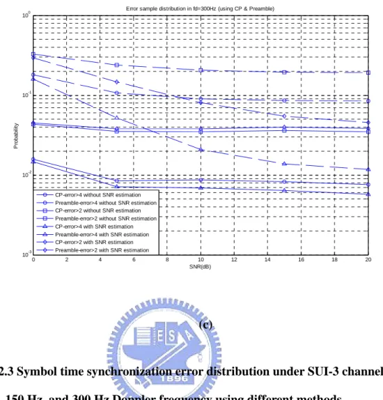
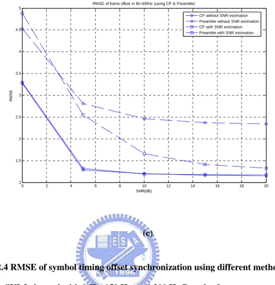
Fig. 2.3 shows how different SNRs affect the error distributions of symbol timing during the two methods with different estimator in various Doppler frequencies. First, in fd = 0 Hz, the channel is almost fixed, we see that the symbol timing estimation is more accurate than mobile channel in fd = 150 Hz and fd = 300 Hz. Second, we compare with the two symbol timing estimation methods using preamble and CP. According to the error probability shown in Fig. 2.3, we observe the probability density function (PDF) of a realistic symbol timing estimate has a large variance in CP correlation method. This is because the preamble conjugate symmetry correlation has a sharper boundary and stronger noise resistance than CP correlation as in Fig. 2.2. Last, we test the performance of estimator (2.6) and find that it has a better performance in high SNR when using CP correlation method. It is likely the CP correlation is sensitive to noise and the estimator (2.6) with SNR estimation can eliminate the noise effect. When using the preamble conjugate symmetry correlation, the estimator (2.6) has almost no effect to performance. The reason is given above. The same simulation results are shown in Fig. 2.4 where the root mean square error (RMSE) is defined

as 2 E n n ∧ ⎧ ⎫ ⎪ − ⎨ ⎪ ⎪ ⎩ ⎭ ⎪

⎬ and we can see which one has better performance. Further, because the

preamble length is longer than CP, larger correlation values improve performance, but also increase the amount of computation required. As a whole, the symbol timing estimation method using preamble has better performance than using CP correlation. But when we take implementation into account, the CP correlation is more suitable for the estimation. The reasons and comparison results are discussed in the next chapter (section 3.3.3).

0 2 4 6 8 10 12 14 16 18 20 10-2

10-1 100

Error sample distribution in fd=0Hz (using CP & Preamble)

SNR(dB) P rob abi li ty

CP-error>1 without SNR estimation Preamble-error>1 without SNR estimation CP-error=0 without SNR estimation Preamble-error=0 without SNR estimation CP-error>1 with SNR estimation Preamble-error>1 with SNR estimation CP-error=0 with SNR estimation Preamble-error=0 with SNR estimation

(a) 0 2 4 6 8 10 12 14 16 18 20 10-3 10-2 10-1 100

Error sample distribution in fd=150Hz (using CP & Preamble)

SNR(dB) P rob abi li ty

CP-error>4 without SNR estimation Preamble-error>4 without SNR estimation CP-error>2 without SNR estimation Preamble-error>2 without SNR estimation CP-error>4 with SNR estimation Preamble-error>4 with SNR estimation CP-error>2 with SNR estimation Preamble-error>2 with SNR estimation

0 2 4 6 8 10 12 14 16 18 20 10-3

10-2 10-1 100

Error sample distribution in fd=300Hz (using CP & Preamble)

SNR(dB) P rob abi li ty

CP-error>4 without SNR estimation Preamble-error>4 without SNR estimation CP-error>2 without SNR estimation Preamble-error>2 without SNR estimation CP-error>4 with SNR estimation Preamble-error>4 with SNR estimation CP-error>2 with SNR estimation Preamble-error>2 with SNR estimation

(c)

Fig. 2.3 Symbol time synchronization error distribution under SUI-3 channel with 0 Hz, 150 Hz, and 300 Hz Doppler frequency using different methods.

0 2 4 6 8 10 12 14 16 18 20 0 1 2 3 4 5 6

RMSE of frame offset in fd=0Hz (using CP & Preamble)

SNR(dB)

RM

S

E

CP without SNR estimation Preamble without SNR estimation CP with SNR estimation Preamble with SNR estimation

(a) 0 2 4 6 8 10 12 14 16 18 20 1 1.5 2 2.5 3 3.5 4 4.5 5

RMSE of frame offset in fd=150Hz (using CP & Preamble)

SNR(dB)

RM

S

E

CP without SNR estimation Preamble without SNR estimation CP with SNR estimation Preamble with SNR estimation

0 2 4 6 8 10 12 14 16 18 20 1 1.5 2 2.5 3 3.5 4 4.5 5

RMSE of frame offset in fd=300Hz (using CP & Preamble)

SNR(dB)

RM

S

E

CP without SNR estimation Preamble without SNR estimation CP with SNR estimation Preamble with SNR estimation

(c)

Fig. 2.4 RMSE of symbol timing offset synchronization using different methods under SUI-3 channel with 0 Hz, 150 Hz, and 300 Hz Doppler frequency.

2.3.2 Fractional CFO Estimation

One of the main drawbacks of OFDM is its sensitivity to carrier frequency offset (CFO). The degradation is caused by two main phenomena: reduction of amplitude of the desired sub-carrier and ICI caused by neighboring carriers described in [1] and [2]. The amplitude loss occurs because the desired sub-carrier is no longer sampled at the peak of the sinc-function of DFT. Adjacent carriers cause interference, because they are not sampled at the zero-crossings of the sinc-functions.

CFO can be partitioned into the fractional part of “normalized CFO” (where normalization is with respect to the sub-carrier spacing) and integral part of “normalized CFO”. We call them “fractional CFO” and “integer CFO” respectively in this thesis.

After obtaining the fine time synchronization, the CFO can be estimated using a 2-step process. During the first step, the receiver estimates fractional CFO by measuring the phase of the CP correlation to avoid ICI before switching to the frequency domain operations. The integer CFO can then be measured in frequency domain using the cross correlation with known preamble sequence, by measuring sub-carrier shift in frequency domain. We talk about integer CFO in the next section.

From [1] and [9], the fractional CFO can be estimated using CP correlation XCP(n)

as 1 * ( ) cp ( ) ( ) n N CP i n X n r i r i + − = =

∑

where Ncp is the length of CP, r(i) is the received signal, and N is the FFT size. This yields the ML estimation of fractional CFO

{

}

{

}

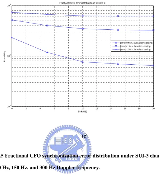
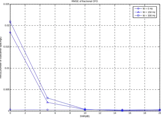
Performance results for the SUI-3 channel in Doppler frequency 0Hz, 150Hz, and 300Hz are shown in Fig. 2.5 and Fig. 2.6. We set the central frequency is 2.5G Hz and the fractional CFO is 2ppm of it. Note that we do not take sampling inaccuracy caused by the sampling frequency offset into account in our simulation. Fig. 2.5 shows how SNR affects the error distribution of carrier frequency synchronization. In fd = 0 Hz, the channel has no Doppler spread, its performance is better than fd = 150 Hz and fd = 300 Hz and has no error floor. It is found that when SNR = 10 dB in the mobile channel, the correct frequency offset under 2% of the sub-carrier spacing (as required

by IEEE 802.16e described in 2.2.3) is more than 90% of all test cases. We can also see

the same results by the way of calculating RMSE defined as

2 E ε ε ∧ ⎧ ⎫ ⎪ − ⎨ ⎪ ⎪ ⎩ ⎭ ⎪ ⎬ in Fig. 2.6.

0 2 4 6 8 10 12 14 16 18 20 10-5 10-4 10-3 10-2 10-1 100

Fractional CFO error distribution in fd=0Hz

SNR(dB) P rob abi li ty

|error|>0.5% subcarrier spacing |error|>1% subcarrier spacing |error|>2% subcarrier spacing

(a) 0 2 4 6 8 10 12 14 16 18 20 10-3 10-2 10-1 100

Fractional CFO error distribution in fd=150Hz

SNR(dB) P rob abi li ty

|error|>0.5% subcarrier spacing

|error|>1% subcarrier spacing

|error|>2% subcarrier spacing

0 2 4 6 8 10 12 14 16 18 20 10-2

10-1 100

Fractional CFO error distribution in fd=300Hz

SNR(dB) P rob abi li ty

|error|>0.5% subcarrier spacing |error|>1% subcarrier spacing |error|>2% subcarrier spacing

(c)

Fig. 2.5 Fractional CFO synchronization error distribution under SUI-3 channel with 0 Hz, 150 Hz, and 300 Hz Doppler frequency.

0 2 4 6 8 10 12 14 16 18 20 0 0.005 0.01 0.015 0.02 0.025

RMSE of fractional CFO

SNR(dB) R M S E (num b e r of s u bc arri e r s pac ings ) fd = 0 Hz fd = 150 Hz fd = 300 Hz

Fig. 2.6 RMSE of fractional CFO synchronization under SUI-3 channel with 0 Hz, 150 Hz, and 300 Hz Doppler frequency.

2.3.3 Integer CFO Estimation and Preamble Index

Identification

After time and frequency synchronization in time domain, we do the integer CFO estimation and the preamble index identification in frequency domain (see Fig. 2.1). Since the preamble index must be estimated by using the preamble, we keep the received preamble signal in a buffer after the FFT function block. Then we estimate the integer CFO and identify the preamble index using the compensated preamble in the frequency domain.

Note (1.1) in 1.3.2 there are three types of preamble carrier-sets and each segment uses only one carrier-set. As the feature of the preamble, we cannot find the exact

integer CFO until we find the correct preamble index which contains the information about the used carrier-sets and vice versa. Directly we consider the brute force correlation method to find the preamble index and integer CFO jointly. Fortunately since the preamble data is BPSK (1-bit) in frequency domain, it allows easier implementation without any need for complex multipliers. Further reduction in complexity can be achieved with the knowledge that the preamble is transmitted on every 3rd sub-carrier.

Refer to [8] the joint integer CFO and preamble search can be summarized as

1 ₂ , ₀ , arg max N ( ) _i m( ) i m _k i m R k P k − ∧ ∧ = ⎛ = _⎜ ⎝

∑

where m∈

{

}

{

}

i∈ −Nfo +Nfo represents the range of integer CFO, R is the received preamble

symbol in frequency domain (as estimated by time acquisition step), Pm is the m-th

possible preamble sequence, Nfo is the maximum frequency offset normalized to sub-carrier spacing, and ( )v n _idenotes the shift of vector v(n) by i elements.

Further, in order to reduce the number of correlation operations, we present a method using the guard band power of preamble to do the coarse estimation of integer CFO first and than do the preamble index identification. We observe the sub-carrier structure of different segments near the guard band from Fig. 2.7. When the segments are 0, 1, 2, the corresponding sub-carrier permutations are shown in the top, middle, bottom of Fig. 2.7, respectively. All 114 preambles are classed as three segments (carrier-sets) described in (1.1). The method of coarse integer CFO estimation using guard band power calculation and preamble index identification is described as follows.

(2) Set a window which length is the same as guard band range. Then calculate the signal power inside the window and shift the window to find the sub-carrier permutation fit in with the segment 0 (top of Fig. 2.7). The amount of the window shift fitting segment 0 is the coarse integer CFO. (3) Compensate the coarse integer CFO.

(4) Calculate the correlation of frequency domain received preamble compensated by coarse integer CFO and all segment 0 preambles using (2.9). Because we do the coarse integer CFO we can reduce the search range Nfo of

i in (2.9). Set a threshold and find the maximum correlation value exceeding

it. The preamble index and final correct integer CFO are our goal.

(5) If we can not find a maximum correlation value exceed the threshold, it means that there is no correct preamble index in all segment 0 preambles. We return to (1) and test segment 1 situation from (2) to (4). If it still can not find a correct result, return to (1) and test segment 2 from (2) to (4) until find the true integer CFO and preamble index.

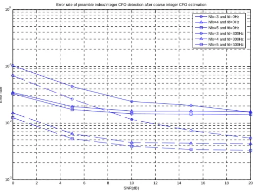
Fig. 2.8 shows the simulation results of the method described above in different Doppler frequencies with FFT size 512 where “error” means incorrect identification of the integer CFO or the preamble index or both. We discuss the influence of the search range Nfo selection after the coarse integer CFO estimation. From Fig. 2.8, the results for Nfo = 4 and Nfo = 5 are almost the same and better than Nfo = 3. So setting the search range Nfo for 5 is appropriate to our simulation enough.

0 2 4 6 8 10 12 14 16 18 20

10-3 10-2 10-1 100

Error rate of preamble index/integer CFO detection after coarse integer CFO estimation

SNR(dB) E rror rat e Nfo=3 and fd=0Hz Nfo=4 and fd=0Hz Nfo=5 and fd=0Hz Nfo=3 and fd=300Hz Nfo=4 and fd=300Hz Nfo=5 and fd=300Hz

Fig. 2.8 Error probability of preamble index identification after coarse integer CFO estimation under SUI-3 channel with different Doppler frequencies and search range.

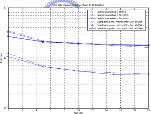
Now we compare the performance and computational complexity of the two methods described above. Assume that the symbol timing and fractional CFO offset are perfect estimated and compensated. Set the maximum search range of integer CFO to be ±10Δf , and let the preamble index be 31 in our simulation. Fig. 2.9 shows the

error probability of 105 test samples under SUI-3 channel in various SNRs and Doppler frequencies with FFT size 512. The brute force correlation method has a little better performance than guard band power calculation method in low SNR. This is because the guard band power is led by the noise. There is only noise power in the guard band so that we may not find the sub-carrier pattern shown in Fig. 2.7 accurately and make a worse coarse integer CFO estimation. The true integer CFO is probably outside the search range and the preamble identification failed. In high SNR, the performance of the two methods is almost the same and does not improve more, i.e. it has an error floor. It is because the noise is independent and has no effect on the signal correlation. Further, the threshold setting has some influence on performance.

0 2 4 6 8 10 12 14 16 18 20

10-3 10-2 10-1

Error rate of preamble index/integer CFO detection

SNR(dB) E rro r r a te Correlation method in fd=0Hz Correlation method in fd=150Hz Correlation method in fd=300Hz Guard band power method (Nfo=5) in fd=0Hz Guard band power method (Nfo=5) in fd=150Hz Guard band power method (Nfo=5) in fd=300Hz

Fig. 2.9 Error probability of either the estimated integer CFO or the identified preamble index under SUI-3 channel with different methods.

We analyze the computational complexity. The major load of complexity is the

number of multiplications. There are 114 142 21×

(

)

multiplications for the brute force correlation method where 114 is number of all preambles, 142 is the number of BPSK PN symbols used in preamble, and 21 (Nfo=10) is the estimation range of integer CFO. For the guard band power calculation method,

there are 76 complex multiplications used where 76

( (142 11) 118712 × × = 1 114 1 114 1 114 2 3 3 3 3 3 3

= × + × × + × ×3) is the expect number of the preambles used to

calculate in the method and 11 (Nfo=5) is the search range of integer CFO. Note that the guard band power method has lower complexity. The complexity reduction is depended on the search range Nfo but make sacrifice for performance in low SNR. Allow for the better performance, the correlation method is maybe more suitable to find the preamble index and integer CFO jointly in IEEE 802.16e.

Chapter 3

DSP Implementation of IEEE

802.16e Downlink System

DSP implementation is the final goal of our work. The MSC8126ADS board (see Fig. 3.1) is made by Freescale Semiconductor. In this chapter, we introduce the architectures of the DSP board.

This chapter is organized as follows. In section 3.1, we present the architecture of the MSC8126ADS board. In section 3.2, we introduce that how to develop optimized code for speed on the SC140 cores.

3.1 Introduction to the DSP Platform

3.1.1 MSC8126ADS Board Architecture

The MSC8126ADS board uses the Freescale MSC8126 processor [10], a highly integrated system-on-a-chip device containing four StarCore SC140 DSP cores along with an MSC8103 device as the host processor. The MSC8126ADS board serves as a platform for software and hardware development in the MSC8126 processor environment. Developers can use the on-board resources and the associated debugger

to perform a variety of tasks, such as downloading and running code, setting breakpoints, displaying memory and registers, and connecting proprietary hardware via the expansion connectors. This board works seamlessly with the CodeWarrior Development Studio for StarCore. According to [10], we described the MSC8122/26ADS board features in Table 3.1 as follows.

Table 3.1 MSC8126ADS Board Features

Feature Description

MSC8126ADS board

• Host debug through a single JTAG connector supports both the MSC8103 and MSC8126 processors.

• MSC8103 is the MSC8126 host. The MSC8103 system bus connects to the MSC8126 DSI.

• Emulates MSC8126 DSP farm by connecting to three other ADS boards.

3.1.2 MSC8126 Features

The MSC8126 (see Fig. 3.2) is a highly integrated system-on-a-chip that combines four SC140 extended cores with a turbo coprocessor (TCOP), a Viterbi coprocessor (VCOP), an RS-232 serial interface, four time-division multiplexed (TDM) serial interfaces, thirty-two general-purpose timers, a flexible system interface unit (SIU), an Ethernet interface, and a multi-channel DMA controller.

The SC140 extended core (see Fig. 3.3) is a flexible, programmable DSP core that handles compute-intensive communications applications, providing high performance, low power, and code density. It efficiently deploys a novel variable-length execution set (VLES), attaining maximum parallelism by allowing multiple address generation and data arithmetic logic units to execute multiple operations in a single clock cycle. A single SC140 core running at 500 MHz can perform 2000 MMACS. Having four such cores, the MSC8126 can perform up to 8000 MMACS per second.

Based on [11], we organized the features of MSC8126 and SC140 extended core and listed them in Table 3.2. The block diagram of the MSC8126 is shown in the Fig. 3.2 and SC140 extended core is shown in the Fig. 3.3.

Table 3.2 MSC8126 Features Feature _Description

MSC8126

• Four-core DSP with internal clock up to 500 MHz at 1.2 V. System bus frequency up to 166 MHz using 64 or 32 data lines, addressing up to 4 GB external memory,

connected to:

— 16 MB of soldered, non-buffered on one 4-bank × 1 M × 32-bit device.

— 4 MB of buffered Flash memory organized as 4 M × 8-bit for configuration/boot/program storage.

•DSI frequency up to 100 MHz as a 32-bit or 64-bit slave on the MSC8103 system bus connects to:

— 2 MB of non-buffered SDRAM organized as 32-bit (default) or 64-bit.

— 16 MB of 100 MHz soldered, non-buffered SDRAM, organized on two 4-bank × 32-bit devices.

— 4 MB of 16-bit buffered Flash memory.

— Buffered board control and status register (BCSR) with eight byte-sized registers.

•SDRAM machine controls the SDRAM on the system bus. •SMII support for MAC-to-PHY or MAC-to-MAC connections. •RMII and MII support for MAC-to-PHY connections.

•Core power level adjustable via potentiometer. •Includes Viterbi coprocessor and Turbo coprocessor.

3.1.3 Developing Optimized Code for Speed on SC140

Cores

Speed optimization techniques on the SC140 core reference to [12] are generally classified as follows.

z Loop unrolling

the body of a loop with corresponding indices. As a stand-alone technique, loop unrolling increases the Data ALU usage per loop step. If the iterations are independent, each one is performed on a single Data ALU.

z Split computation

A frequent operation in DSP computations is to reduce one dimension of a data massive (scalars are zero-dimensional, vectors are one-dimensional, and matrices are two-dimensional). The most frequently used reductions are: energy computation of a vector, mean square error, or maximum of a vector. If the reduction operator is associative and commutative, the reduction can be performed by splitting the original data massive into several data massives (usually four on the SC140 core).

The same conditions must be met as for loop unrolling (for example, the vector alignment and the loop counter). In addition, split computations are used if the operator on the given data set is associative and commutative.

z Multisampling

The multisampling technique is frequently used in nested loops and is a combination of primitive transformations. Given a nested loop formed out of OL (outer loop) and IL (inner loop containing one or two instructions), the multisampling transformation consists of the following.

(1) A loop unroll applied for OL to create a new OL with four IL inside (IL0, IL1, IL2, and IL3).

(2) A loop merge applied for IL0, IL1, IL2, and IL3 to create a new IL that makes more efficient use of the DALU units.

(3) A loop unroll applied to the newly-obtained IL so that the programmer can detail the reuse of already fetched values in the computations inside the new IL.

The speed increases by sample-factor times, but the code size also increases significantly. Therefore, multisampling should be used only if the speed constraints are

much more important than the size constraints.

3.2 Implementation of Transmitter

Our IEEE 802.16e OFDMA downlink PHY implementation system on the MSC8126 includes the user domain processing (UP), the frequency domain (FP) processing, and the time domain processing (TP). The following diagram, Fig. 3.4, gives a high level view on the main building blocks for WiMAX OFDMA PHY processing. The upper PHY part on the MSC8126 includes the two main subsystems UP and FP. The demo focuses on the data path implementation, assuming a fully synchronized system. Tx User SP Tx User SP Rx Time Domain SP Tx Time Domain SP Tx User SP Rx User SP D/A A/D A na log stag e s Uplink Rx PHY Tx Frequency Domain SP Rx Frequency Domain SP Tx Time Domain SP Rx Time Domain SP Downlink Tx PHY MAC L a yer IF 1TX IF 2TX IF 3TX IF 4TX IF 4RX IF 3RX IF 2RX IF 1RX

Fig. 3.4 WiMAX PHY interfaces.

The user domain processing covers the channel encoding and decoding steps. Specifically these are:

z Randomization and derandomization z Convolutional encoder and decoder

z Interleaving and deinterleaving

z Constellation mapping and demapping

Fig. 3.5 shows an overview of the UP steps throughout the PHY chain on the MSC8126. Random izer FE C Encoder E d Interleaver Q P SK Modulation M AC layer TX UP Fig. 3.5 DL UP chain on MSC8126.

The frequency domain processing is mainly responsible for the OFDMA signal formatting. It is a subsystem that is not tied to any specific user functionality. The processing steps in the DL direction are:

z Preamble generation z Data modulation z Data symbol mapping

z Pilot generation and mapping z Carrier scrambling

From a processing point of view, the DL FP data flow is as follows and shown in Fig. 3.6.

(1) The first symbol in a frame is the preamble, which is a PN code pattern dependent on some control variable like ID cell. It is independent of user data. The mobile station knows this sequence and hence may use for initial

channel estimation.

(2) After the preamble user processing fills sub-channels with user and control data. FP performs as follows and is shown in Fig. 3.7 for detail.

z Mapping data to logical slots on logical sub-channels (function MapDl()).

z Generate and insert the pilot symbols into the tiles.

z Translate the logical carriers to physical carriers by the function CarrierScrambler(). This function needs a permutation table which is generated by GenerateDlTable(). This map is generated once per permutation zone.

z Modulate the resulting data vector on the physical carriers by a PN sequence and a static weight. This is achieved by the function DataModulation().

MapDl()

Map user bursts on frames in the symbol sub-channel space

(see [1..3]. sec 8.4.3.4)

CarrierScrambler()

Scramble carrier by using look-up table

To IFFT From DL User processing

Carrier Lookup table:

ausiDlCarrierMap[] GenerateDlTable(..)

Generate Carrier Lookup Table (see [1..3]. sec 8.4.6.1.2.2.2) Map Information PreambleGen() Preamble Generation (see [1..3]. sec 8.4.6.1.1) From DL User processing Map Information To IFFT DataModulation() RCF-IF MapToComplexRowVec tor()

N-Used/ 14 adjacent Carriers 14 adjacent Carriers = 14 adjacent Carriers 14 adjacent Carriers 14 physical Cluster 14 adjacent Carriers 14 adjacent Carriers = 14 adjacent Carriers 14 adjacent Carriers N-Used/14 locical Cluster First Perm Formula: Cluster Scrambling Major Group 0 Major Group 5 locical Cluster 0-> N-1 locical Cluster 5N-> 6N-1 N=24 for FFT2048 N=12 for FFT1024 N=10 for FFT512 N=2 for FFT128 N-Used physical Carriers Linear ordered data carriers All Carriers except pilots All Carriers except pilots Second Perm Formula: Carrier Scrambling Linear ordered data samples DL User Processing Physical to logical

Fig. 3.7 DL carrier scrambling scheme.

The time domain processing includes IFFT/FFT and synchronization mechanism. In our DSP implementation programs, it is limited to only PUSC and the configurations marked as “optional” in [4] and [5] are not considered. This functionality is confined to user independent sub-channel management. Hence, all specific control channels like ranging, FCH, Map-DL/UL bursts etc are not considered specifically because they are treated as normal bursts. Table 3.3 and Table 3.4 list the cycle count of UP and FP respectively for WiMAX OFDMA DL transmitter on single MSC8126 SC140 core running up to 500 MHz. Fig. 3.8 and Fig. 3.9 show the histograms of them. In DL UP, we see Fig. 3.8 and obtain that the interleaver and modulation spend clock cycles about 50 % of total respectively. To speed up implementation, the functions using shift registers or memory arrangement like randomizer, convolutional encoder, puncture, and interleaver are written by assembly language and the improvement of cycle count is shown in Table 3.3. In DL FP, we

transmit the preamble and a data symbol which needs to execute the initialization function. Then record clock cycles of every function using in the preamble and data symbols as Table 3.4. Fig. 3.9 shows the histogram of all FP functions. Clearly, we see that the preamble spends fewer clock cycles and the data initialization spends most clock cycles. Fortunately, the data initialization must be done only once in a data burst. So it doesn’t spend much time to transmit data symbols and the real time speed is

about 20842 symbols per second ( 500 ( / sec)

23990( / )

M cycles cycles symbol

Table 3.3 Cycle Count of DL UP

Function Cycle Count (cycles/bit)

Randomizer (assembly) 0.15

Randomizer 0.23

Convolutional Encoder (assembly) 1.02

Convolutional Encoder 2.21

Puncture (Rate = 1) (assembly) 0.45

Puncture (Rate = 1) 0.71

Interleaver (assembly) 13.64

QPSK Modulation 15.95

Total Cycles (assembly) 18.59

Bit Rate (Mbits/sec) 26.39

Cycle count of UP functions

0 2 4 6 8 10 12 14 16 18 20 C lo ck cy cl es p er b it Randomizer (assembly)

Convolutional Encoder (assembly) Puncture (Rate = 1) (assembly) Interleaver (assembly)

QPSK Modulation Total Cycles

Total

Table 3.4 Cycle Count of DL FP

Function Description Function Name Cycle Count

Preamble

Symbol Preamble Generation PreambleGen() 4175

Carrier Permutation Table

Generation GenerateDlTable() 98089

Initial Data Position within

Sub-channel InitialDataPositionVectorDl() 1360

Data Initialization

Subtotal Cycles 99508

Mapping Data onto Physical

Sub-carrier MapDl() 3147

Carrier Scramble CarrierScramble() 5661

Carrier Manipulation DataModulation() 10945

Data Symbol

Subtotal Cycles 23990

Total Cycles 135549

Data Symbol Rate (symbols/sec) 20842

Data Rate (Mbits/sec) 17.51

Cycle count of FP functions

0 20000 40000 60000 80000 100000 120000 140000 160000 C lo ck cy cl es PreambleGen() GenerateDlTable() InitialDataPositionVectorDl() MapDl() CarrierScramble() DataModulation() Total

3.3 Performance Analysis of Synchronization

Implementation

We implement initial synchronization techniques described in section 2.3 for WiMAX OFDMA downlink on MSC8126 DSP. All simulation parameters and environments are similar to those in chapter 2, but we translate floating data type to short integer data type. For comparison, floating point simulation results are also presented together with the fixed point results.

3.3.1 Symbol Timing Estimation

As the description in section 2.3.1, we use the preamble to estimate the symbol timing offset. Fig. 3.10 shows the RMSE of symbol timing offset estimation in SUI-3 channel for different Doppler frequencies. We can see the curves of fixed point simulation are very close to those of floating point simulation.

0 2 4 6 8 10 12 14 16 18 20 0.5 1 1.5 2 2.5 3 3.5 4 4.5 5 5.5

RMSE of frame offset in fd=0Hz

SNR(dB) RM S E floating point fixed point (a) 0 2 4 6 8 10 12 14 16 18 20 1 1.5 2 2.5 3 3.5

RMSE of frame offset in fd=150Hz

SNR(dB) RM S E floating point fixed point (b)

0 2 4 6 8 10 12 14 16 18 20 1 1.5 2 2.5 3 3.5

RMSE of frame offset in fd=300Hz

SNR(dB) RM S E floating point fixed point (c)

Fig. 3.10 RMSE of symbol timing offset synchronization under SUI-3 channel.

3.3.2 Fractional CFO Estimation

When implementing the fractional CFO estimation on MSC8126 DSP platform we have a difficulty to obtain the phase of CP correlation. Taking hardware signal processing complexity into account, we adopt a phase estimation algorithm which is called CORDIC, an acronym for COordinate Rotation DIgital Computer. This algorithm described in [13] for detail provides an iterative method of performing vector rotations by arbitrary angles using only shifts, adds and a small lookup table. So it is a better choice to use in the fixed point environment on DSP platform. For our implementation on MSC8126, the phase of the CP correlation value which represents

the frequency offset is normalized byπand it is between [-1,…,+1) with Q15 format (16 bits).

Fig. 3.11 shows the RMSE of fractional CFO estimation in SUI-3 channel for different frequencies. We can learn how the SNR affects the carrier frequency synchronization and see that the corrected frequency offset is under 2% of the sub-carrier spacing, as required by IEEE 802.16e. From the figure on fractional CFO estimation results, we can also see the performance curves for fixed point and floating point implementations are almost the same.

0 2 4 6 8 10 12 14 16 18 20 0 0.005 0.01 0.015 0.02 0.025

RMSE of fractional CFO

SNR(dB) R M S E (num b e r of s u bc arri e r s pac ings ) floating point in fd=0Hz floating point in fd=150Hz floating point in fd=300Hz fixed point in fd=0Hz fixed point in fd=150Hz fixed point in fd=300Hz

Fig. 3.11 RMSE of fractional CFO synchronization under SUI-3 channel with 0 Hz, 150 Hz, and 300 Hz Doppler frequency comparing with fixed point and floating point.