A P P E N D I X
The analytical model of the large-angle magnetic suspension test facility is
AmX + D,«W
y = c„x
( A l ) (A2) where x= CM, A„ = [;=« X?]- B„ = LT'^ and C,„ = [C, Osxs]. The state variable Xp includes pitch and yaw angles and three linear displacements of the cylinder's centroid. The matri-ces A21, A22, S2, and C, are
The eigenvalues of the system matrix A,„ are ±58.78, ±57.81, ±9,78, ±;7.97, and ±;'0.96. The matrix C, which relates the sensor output voltage to the displacement can be obtained from calibration and is assumed known. To recover the displacement from the sensor output voltage, one can use Xp = C'i'y.
The performance index for the state feedback design is chosen as
PI- = Z ylQyk + u'kRu, (A3) where Q = (Ci
—
hx5-V diag [l.e3 l.e3 2.e8 2.e8 2.e8]Cr' and R
A21 = fi2 =
c, =
•3.3415e + 03 0 -9.8070e + 00 -3.6031e - 15 .-2.3357e - 16 3.8370e + 01 0 2.2144e - 01 0 0 3.3415e + 03 -2.4664e - 15 1.9618e - 15 -3.6031e - 15 3.8370e + 01 8.9802e + 01 -1.5274e - 01 1.2154e - 01 -3.9392e + 04 -4.9534e - 12 4.9937e + 01 4.3604e - 15 -2.5089e - 02 4.9534e - 12 4.8609e - 12 4.3604e - 15 9.5577e + 01 -9.0007e - 15 2.081 le - 12 • -1.4472e - 11 -2.5089e - 02 -9.0007e - 15 -9.1324e - 01.3.8370e + 01 3.8370e + 01 3.8370e + 01 ' 5.5514e + 01 -5.5514e + 01 -8.9802e + 01 7.8453e - 02 7.8453e - 02 -1.5274e - 01 -1.9674e - 01 1.9674e - 01
.-2.7672e - 01 -8.5465e - 02 2.2388e - 01 2.2388e - 01
-1.2154e - 01 -8.5465e - 02. 8.9024e + 01 0 -1.1625e + 02 0 0 0 0 0 9.5425e + 01 -1.0725e -I- 02 0 7.8740e 0 0 0 + 03 0 0 0 -6.5359e -5.1813e 03 03 6.097 6e + 03 0 6.2500e + 03 0 0
Feedforward and Feedback Control
Strategy for Active Noise
Cancellation in Ducts
Jwu-Sheng Hu^
This paper presents the theoretical work about active noise cancellation in ducts. The proposed control system is designed based on the assumption of a one-dimensional sound field. The controller consists of a feedforward block which serves as a noise observer. The feedback portion of the control algorithm is to minimize residual disturbances. Closed-loop stability of the MIMO (multiple-input-multiple-output) system is analyzed and the result shows that the dynamic influenced by the space-feedforward and feedback controllers can be decoupled. Both
semi-infinite and finite-length ducts are considered in this study and simulation examples are given to illustrate the effectiveness of the proposed controllers.
1 Introduction
Active Noise Control (ANC) utilizes the physical principle of wave superposition to attenuate unwanted noise. During the
' Associate Professor, Institute and Department of Control Engineering, Na-tional Chao-Tung University, 1001 Ta Hsueh Road, Hsinchu, Taiwan.
Contributed by the Dynamic Systems and Control Division of THE AMERICAN SOCIETY OF MECHANICAL ENGINEERS . Manuscript received by the DSCD July 28, 1993. Associate Technical Editor: M. Dahleh.
past decade, much progress has been reported toward applying ANC to attenuate noise in confined spaces. A review by Nelson and Elliott (1992) presents the fundamental principles underly-ing modem techniques for ANC while Gorden and Vinunderly-ing (1992) provide an overview of the field. The most successful application so far is to cancel noise in ducts, especially cancella-tion of plane waves. Utilizing the principle of wave propagacancella-tion, the active controller can be synthesized by introducing delay elements (Eghtesadi and Leventhall, 1982; Guicking and Karcher, 1984). Although the idea is not new, a complete theo-retical analysis on its performance and closed loop stability has not been presented, especially in a finite-length duct without prior knowledge of the noise source (Trinder and Nelson, 1983). The concept of controlling wave propagation is also investigated in structural vibration suppression (von Flotow and Shafer, 1986; von Flotow, 1986; Pines and von Flotow, 1990; Tanaka and Kikushima, 1992). The problem is more compli-cated because of the distributed-delay dynamic of the plant.
In this paper, theoretical studies about noise cancellation in semi-infinite and finite-length ducts are presented. While many ANC research are conducted in the Fourier Transform domain, the proposed controllers are designed using the Laplace Trans-form so as to avoid causality problem (Curtis et al., 1987) and to analyze closed loop stability. The plant is derived by assuming a one-dimensional sound field in ducts (Hu, 1993). The control-lers' structures are explained by analyzing the interconnection of delay elements in the plant model. For a semi-infinite duct, an upstream microphone is used to observe noise propagating in the downstream direction. This signal is then fed into the controller as a space-feedforward command to attenuate noise transmitting downstream. Theoretically, complete cancellation can be achieved through this control configuration. An addi-tional microphone placed at a downstream location to pick up
x=0 '*Joise Source \ \ "2 _ feedforward Vlicrophones /I
f ^
a X3 Feedback Microphone Ii
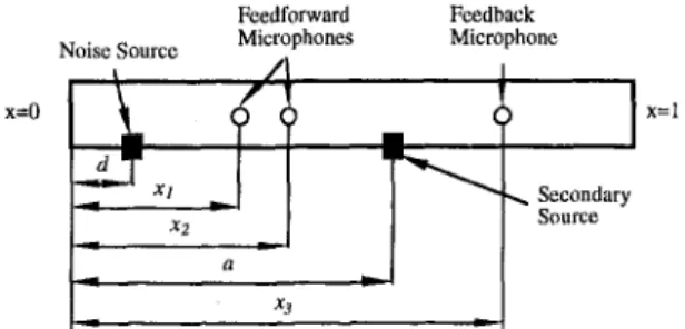
— -^ Secondary Source GD(X, a, s) — --Qi{s)e -iUlc)l2-x~a) X=lFig. 1 Schematic diagram of a finite-length duct (all the variable are dimensionless)
any residual noise is used to generate a feedback signal. Closed-loop stability of the MIMO (multiple-input-multiple-output) system is analyzed and the result shows that the dynamic influ-enced by the space-feedforward and feedback controllers can be decoupled.
For a finite-length duct, the duct's dynamic becomes more complicated due to reflection from the downstream boundary. Consequently, two upstream microphones are needed to observe noise propagating downstream. Unlike the semi-infinite duct, only asymptotic cancellation can be achieved in a finite-length duct using the proposed control strategy. The error dynamic is governed by the characteristic equation of the open loop plant. A complete analysis of the closed loop system including a feed-back microphone is also presented.
It should be noted that the objective of the work is to develop a theoretical foundation of noise cancellation based on wave propagation principles and close-form solutions in the Laplace Transform domain. Other important issues such as the ro-bustness of the control system and actuator and sensor dynamics will be considered in the following studies.
2 The Dynamic Model of a Finite-Length Duct
The schematic diagram of a finite-length duct is shown in Fig. 1. It is assumed that the noise (primary source) enters the duct eA d, & control speaker (secondary source) is placed at a, and X represents a point within the duct. The length of the duct is L and a, d, and x are dimensionless variables. The specific impedance of both ends is denoted as ZQ{S) at J: = 0 and Z\{s) aix — \ where .s is the Laplace variable. It is further assumed that the boundaries are passive. This implies that the impedance functions are positive real (Hu, 1993). Moreover, the pressure reflection coefficients for each end can be defined from the impedance functions as
.(*)
=
1 - Zajs)1 + Zo(i) and ^1(5') =
1 - z i ( ^ ) 1 + zAs) Denoting the strength of the noise and control source as A'(i') and Q{s) respectively, the transfer function of the speaker to the source pressure can be derived as
When rf < X < a, + [Gt,{x, a, s) + G'^x, a, s)]Q{s) + [G^(x,d,s) + Gi(x,d,s)]N{s) (la) and when d ^ a s x, p(x, s) = e„(s)0,(s)e~^''-"''^p(x, s) + [Goix, a, s) + Giix, a, s)]Q(s) + [GUx,d,s) + Gh(x,d,s)]N(s) (lb) where c: speed of sound - 6io(j)(9|(j')e-""'''*''-'*"' (Id) Gu(x, a, s) = -(?-<'-"'•)("-') - 61,(i)e-""'"•'"-"-"> ( l e ) Gtj(x, a, s) = eo(.?)e"*'-'''"'""'" + 6io(.5)6'i(.Oe"''-"''*''''^~"* ( 1 / ) The above equations are obtained from Green's function of a one-dimensional wave equation (Hu, 1993). The superscripts/
subscripts used in the above equations are based on physical meanings of the transfer function. Subscript D means down-stream position, U means updown-stream position, superscript + means pressure wave propagating in the downstream direction, and — means pressure wave propagating in the upstream direc-tion. For example, Gu(x, a, s) represents the influence of the source at downstream position but propagating in the upstream direction. It is easy to see that GD(X, a, s) consists of a direct propagating wave (the first term on the left-hand side) and a wave reflected from the boundary x = 0 (the second term). Further, the multiplication of &o(s) in the second term shows that part of the energy is absorbed by the passive boundary. Notice that a delayed superposition appears in Eq. ( l a ) and (lb). This term represents the wave traveling twice the length of the duct. If no energy is absorbed at both boundaries (^o(*), 6x(s) = ± 1 ) , the reflected wave will be reinforced and results in resonance at certain frequencies.
The transfer functions defined in Eq. ( I c ) to ( 1 / ) possess some interesting properties. Let JT, y be two arbitrary points and x,y a a, the following relations can be derived.
—G'jj(x, a, s)Gu(x, d, s) + Go(x,d,s)Gi(x,a,s) = 0 ( P I ) ~Grj(x, a, s)Gi(y, d, s) + GUx,d,s)GUy,a,s) = 0 (P2) —Gj}(x, a, s)Gr>(y, d, s) + Gn(x,d,s)GUy,a,s) = 0 (P3) These properties will be used later for constructing a noise observer and controller.
3 Noise Cancellation in a Semi-Infinite Duct
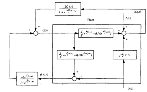
The diagram of a semi-infinite duct is shown in Fig. 2. Its dynamic can be derived from Eq. (1) by letting the impedance at j ; = 1 equal 1 (i.e., zero pressure reflection coefficient). The control signal is derived from the microphone placed upstream (at X2). The purpose of putting another microphone downstream (xi in Fig. 2) will be explained later. Notice that in a semi-infinite duct, we can no longer use dimensionless space vari-ables. Assuming that the effect of noise at X2 is N(s), the pressure response can be written as
Feedforward ,, . „ Microphones Noise Source Feedback Microphone
\ { r ^
— " ' X2 a "1 • ^ j _1
1--•s. Secondary SourcepiX2, S) = 2 ( - « *''' + 6)o(5)e-<"'^'*^2+''>)!2(*) + N(s) (2a) Moreover, the pressure response at any downstream position x > a is
p(x, s) = i(e-("'^«^-'" + 0o(^)e"''"'"*""'"')Q(^)
+ e -(.sIcXx-x.) N(s) {2b) The objective is to block the transmission of noise, i.e., p{x, s) = 0. Solving Qis) by letting Eq. (2b) equal zero, we have
Q(s)
_'2Q-islc){x-x^)
-islc)(.x-a) + Oa(s)e-
7^^i')
Substituting Eq. (2a) into the above equation, the control signal can be shown as
G(*) =
_2g-(.5/c)(a-Xj)
1 + i;^/'^^^,^) (3)
The control law can also be derived by combining Eq. (2a) and (2b):
p(x, s) — e ~(,SIC)(X-X,)
P(X2, S)
An interesting observation of Eq. (3) is that the control signal is independent of the impedance at the boundary. In fact, the result is the same as the case of an infinite duct (Eghtesadi and Leventhall, 1982). From Fig. 2, it is obvious that the purpose of placing a microphone upstream is to detect the noise before it arrives at the position of the cancellation speaker. Therefore, it is characterized as a space-feedforward control signal. Never-theless, in time domain, it is still a feedback control system and the closed-loop response at X2 can be derived as
1 + g-(2.r/c)C<.-X2) p(x2, s) = T^rrr N(s) ^ , 1 + 9o(s)e^'-^"'^" ^
(5)
Equation (5) shows that the cancellation speaker acts like a hard-walled boundary (impedance equals infinity). Since Oo(s) is derived from a passive boundary, the closed-loop system is stable (Hu, 1993).
To accommodate the model uncertainty, a "true" feedback signal should be used in the overall control system. Since the target area is the downstream area of the duct, the error signal measured at Xi(>a) is included in the controller as
Q(s) -2e 1 + e -(slc)(a-x,) -i2.s/cna-x^)P(^^' •^) ~2C(s) 1 + e (2.,/c.)(„-.„)/'(-«l"*) ( 6 ) where C(s) is the feedback compensator. The block diagram of the overall control system is shown in Fig. 3. Suppose some bounded uncertainty S(s) (Fig. 3) is presented at Xi, the re-sponse of p(X[, s) can be shown as
p(xi, s) = 6(s)
1 + C{s)e -(s(,x.-a)/c) (7)
The controller C{s) can be designed to minimize the effect of the disturbance. Since the control system is a multiple-input-multiple-output (MIMO) system, it is essential to analyze the global stability. As will be shown later, the stability is guaran-teed if and only if both Eqs. (5) and (7) are stable. Substituting Eq. (6) into Eq. ( 2 ) , the closed-loop transfer function can be derived as g n ( . 0 8i2(s) 82i(s) g22(s) p(Xi, S) _P(X2, S) N(s) g-(2.,/c)U,-,,)^(^) + 6{S) (8) where g-uic)u,-x^) _ 0 (s)e-'-"'^'-"^'^'> ^, , « n ( j ) = 77-—^n.i.-M,.^r,. C(s) (1 + e~ "T)) g\l(s) = g2x(s) = 1 + gn(s) = (\J^ g-(2s/c)(<"-J;2)\ I _|_ g - ( 2 j / c ) ( < i - j : j ) g - ( . , W U , - . , ) _^ Q^^^^y-i,lc,(x^*^a~x^^ (1 + e-(2"0(<.-'2)) C(s)
It is straightforward to verify that the characteristic equation of the above equation is
(1 + 9o(i)c"*''"'*'')(l + C(s)e -(.s(x,-a)/c) ) = 0 (9)
The condition on C{s) to guarantee stability of the system can be checked by using various frequency domain methods (Marshall, 1979). This condition depends on the value of xj -a. An obvious choice of x, to simplify the design is Xi = a (collocated sensor and actuator).
4 Noise Cancellation in a Finite-Length Duct
The dynamic of sound in a finite-length duct (Section 2) is more complicated than the infinite one. Unlike the semi-infinite duct, the noise travels in the upstream direction due to reflection from the boundary (x = 1 in Fig. 1). As a result, the space-feedforward signal can not be constructed by a single microphone only. To better explain the proposed control system, we first examine the following control law:
G(.)=^gf^iV(.)
GD(X, a, s) (10)
where x > a is a downstream location. Substituting Eq. (10) into Eq. (lb) and using ( P I ) , the pressure response atx satisfies
p(x, s) - 0o(s)di(s)e -(2L,t/c) 'p(x,s) = 0 (11) This means that the pressure will go to zero asymptotically. The proposed control law (Eq. (10)) is derived by letting the controlled sound propagating downstream cancel the noise propagating downstream. Once the downstream-propagating noise is canceled, the upstream-propagating noise will vanish automatically as demonstrated by Eq. (11). The same result can also be obtained at other downstream location y > a. Ac-cording (P2) and (P3), the response at y can be derived. p(y,s)-eo(s)9,(s)e" '^p(y,s)
= [GUy, a, s) + GTAy, a, s)] i ^ ^ ^ " " ' ' ^ ' f N(s) Go(x, a, s)
+ [Gi(y, d, s) + Gi{y, d, s)]Nis) = 0 In order to implement Eq. (10), a noise observer based on microphone measurements has to be constructed. Let two micro-phones be placed at x, and X2 (Fig. 1), from Eq. ( l a ) , the following relation can be derived.
Feedback Controller
o
Q(s) -2e< 1 + e plh'^) -2C(si 1 +e' Plant -'/.>-%ftW.^'""'7 ^/_,-1'-^ftW.>"'76-^
Ftv) S(s) ^ -'l>i- X,) N(s) Space-feedforward ControllerFig. 3 Block diagram of active noise control system in a semi-infinite duct
X [ G J ( x , , a, s)Qis) + GUxu d, s)N{s)] (12a) where
p, = p{xu s) - e,{s)6,(s)e'''^''''^pixu s) {Mb) and
P2 = Pix2, s) - eois)e,is)e^'''^'''>p(x2, s) (12c) Further, the noise propagating downstream satisfies the follow-ing equation.
Gt(x, d, s)Nis) = e-"'~"i'"->^G;(;c,, d, s}N{s) As a result, the downstream noise observer can be designed as
Qis) = - ( p ( x , , s) - p(xi, i)e-(('2-^,)'=)-^')e-(«""'i)'')^' 1 ~i2(x,~i,)/c)U
C(s)p(x3, s)
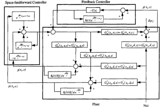
1 - e,(s)e<'^'^'<'-'3' (16) where x^ is a downstream position as indicated in Fig. 1. The complete block diagram of the control system is depicted in Fig. 4 where 5 ( i ) is a bounded uncertainty presented at x^. As shown in the Appendix, the pressure response at x, is
p{Xi, S) = 6(s) [1 -t- C(i')e~<'^''><^5"'"][l - 6»o(*)6'i(.s)e-'^'"'''] (17) Gi(x, d, s)N{s) = -(2(x^-x,)/c)U Giixu a, i)e-"-'--'i'"^'^(2(j) (13) \ — e ' " ' 2 ' I ' -{ix-x.)lc)L!i f
Substituting Eq. {\2b), (12c), and (13) into Eq. (10), the control law becomes
-{p{xu s) - p{x2, ,)e-<(^2-^.v-)^)e-«'--^.)^^)^
It is interesting to see that the control law is independent of the impedance functions at both boundaries. By applying Eq. (14), the pressure response at upstream location is altered. As shown in the Appendix, the pressure response ?Ay,d<y<a,\s piy, s)
1 + 9o(s)e -(2Lslc)a Nis)
(15) As clearly shown in the denominator of Eq. (15), the secondary source acts like a hard-walled boundary. The space-feedforward controller in Eq. (14) is combined with a feedback signal as
Similar to the case of semi-infinite duct, an obvious choice of
^3 is a .
Finally, we examine the closed-loop characteristic equation of the overall system. As shown in the Appendix, the character-istic equation can be derived as
[1 -t- flo(*)e""^''""'][l + C(i)e~<'"'''><-'3-''>]
X [1 - Oo(s)e,(s)e'^^'-'"^] = 0 (18) which consists of the dynamics appeared in Eqs. (15) and (17).
5 Simulation Examples
The following parameters are used to simulate the control system for a semi-infinite duct (Fig. 2 ) .
a = 0.7m, d = O.lm, Xi - 0.7m, Xt = 0.4m, and qo = 0.5. The speed of sound is assumed to be 350 m/s. It is noted that the feedback microphone is placed at the speaker's position (collocated). Figure 5 shows the pressure response of a pure space-feedforward control (assuming S(^s) = 0 ) . The response is measured at x = 2.3m. It can be seen that once the controller is turned on, the pressure at downstream position becomes zero as explained in Section 3. Figure 6 shows the pressure response at A;, when d{s) is not zero and the feedback control law is included. The feedback controller is selected as
Space-feedforward Controller Feedback Controller Jjfjj+a-;jr,J
3
-'',-;> •^c-p(Xj,s) p(x,.s) -C(s) 9,(s)eT
p(Xj,s)o-G:(x„a.s)+a;,(x,.a,s) GJx,.a,sHG;(x„a,s) S(s)
<y-^ i , + Gl(x,.d,s)+Gl(x,,d,s) G„( X2,a,s) +GJ Xj,a,s) 8„(s)e,(s)e
T
GJx„d,s) + GJx,.d,s) eo(s)e,(s)eU-(y* Gl(x„ds) + Gl(x„ds) Plant
Fig. 4 Block diagram of active noise controi system In a finlte-iengtii duct N(s) 0.5
I
I
0.2 0.4 0.6 time (second) 0.8Fig. 5 Pressure response of a pure space-feedforward controi In a semi-Infinite duct (controlier is turned on at t = 0.2 s)
time (second)
Fig. 7 Pressure response of a pure space-feedforward control in a finlte-lengtin duct
Figure 7 shows the result of pure space-feedforward control when 6(s) = 0. The pressure goes to zero asymptotically as indicated by Eq. (11). The same controller C(s) (Eq. (19)) is used to simulate the feedback control. Figure 8 shows the pres-sure response at x^.
6 Conclusion
Active noise cancellation in ducts based on delay relations of wave propagation is discussed. The proposed controllers use
0.2 0.4 0.6 0.8 1 time (second)
Fig. 6 Pressure response of space-feedforward and feedback control in a semi-infinite duct (non-zero disturbance S{s) as shown in Fig. 3)
C(s) 500
i + 100 (19)
The case of sound cancellation in a finite-length duct is also simulated by using the following parameters,
L = 3.13m, a = 0.379, d = 0.076, xi = 0.228, X2 = 0.176, Xj = 0.379, and qa = q\ = 0.5. ! ' « * * * * * « * * ^ ^ 0.5 1 time (second) 1.5
Fig. 8 Pressure response of space-feedforward and feedback control In a flnlte-iengtfi duct (non-zero disturbance S(s) as shown In Fig. 4)
both space-feedforward and feedback sound measurements. It is shown that by carefully selecting the delay elements in the controller, prior information of noise can be observed. Most importantly, the design results in simple closed-loop transfer functions which are easy to analyze. More theoretical develop-ment as well as experidevelop-mental verification will be conducted in future research work.
Acknowledgment
This research work is supported by the National Science Foundation of USA under grant number MSS-9210756.
References
Eghtesadi, Kh. and Leventhall, H. G., 1982, "Active Attenuation of Noi.se— The Monopole System," Journal of Acoustic Society of America, Vol. 71(3), pp. 608-611, Mar,
Curtis, A. R. O., Nelson, P. A., Elliott, S. J. and BuUmore, A. J„ 1987, "Active Suppression of Acoustic Resonance," J. Acoust. Soc. Am., Vol. 81, pp. 624-631.
Gorden, R. T. and Vining W. D., 1992, "Active Noise Control: a Review of The Field,'' American Industrial Hygiene Association Journal, Vol, 53(11), Nov. Guicking D. and Karcher K., 1984, "Active Impedance for One-Dimensional Sound," Journal of Vibration, Acoustic, Stress, and Reliability design. Vol. 106, pp. 393-396, July.
Hu, J., 1993, "Active Sound Cancellation in Finite-Length Ducts Using Closed Form Transfer Function Models," in press, ASME JOURNAL OF DYNAMIC
SYS-TEMS, MEASUREMENT, AND CONTROL.
Marshall, J. E., 1979, Control of Time-Delay Systems, Institution of Electrical Engineers, London.
Nelson, P. A. and Elliott, S. J., 1992, "Active Noise Control: A Tutorial Review," lEICE Trans. Fundamentals, Vol. E75-A, No. U , Nov.
Pines, D . J. and von Flotow, A. H., 1990, "Active Control of Bending Wave Propagation at Acoustic Frequencies," Journal of Sound and Vibration, Vol.
142(3), pp. 391-412.
Tanaka, Nobuo and Kikushima, Yoshihiro, 1992, "Active Wave Control of a Flexi-ble Beam," JSME International Journal, Series m. Vol. 35, No. 2, pp. 236-244.
Trinder, M. C. J. and Nelson P. A., 1983, "Active Noise Control in Finite Length Ducts," Journal of Sound and Vibration, Vol. 89(1), pp. 95-105.
von Flotow, A. H. and Shafer, B., 1986, "Wave-Absorbing Controller for a Flexible Beam," Journal of Guidance, Control, and Dynamics, Vol. 9, No. 6, pp. 673-680.
von Flotow, A. H., 1986, "Traveling Wave Control for Large-Space-Craft Structures," Journal of Guidance, Control, and Dynamics, Vol. 9, No. 4.
A P P E N D I X
Proof of Eq. (15): Defining py as the following
From Eq. ( l a ) , we have:
Py = p{y, s) - eois)dds)e-^''^"^p(y, ,s) (A-1)
Py = [Gtiy, a, s) + Gu(y, a, s)]Q(s) + [GUy, d, s) + G^iy, d, s)]N(s) Using control law of Eq. (10), the following equation can be derived.
Py = -[Gi(y, a, s) + Gd(y, a, s)] ^l^^""' ''' 'l N(s) + [GtAy, d, s) + Goiy, d, s)]N{s)
GD(X, a, s)
G^(v d c'le-f'-^X''''')'
= -[Gaiy, a, s) + Guiy, a, s)] 1Y' ' _,,_,»,;,), N(s) + [GUy, d, s) + Goiy, d, s)]N(s) Gh(y, a, s)e ' yx^'-"-)'
_ [Gi(y, d, s)GUy, a, s) + Gojy, d, s)Gi{y, a, s)]N{s) [Gt(y,a,s)Giiy, d, s) + Gd(y, a, s)Gi(y, d, s)]N{s)
Giiy,a,s) Giiy,a,s) Expanding the numerators in the above equation and rearranging the all terms, we obtain:
[1 - eo(.s)6'i(j')e"<^'-'"'*][e"<'-"'*'''~'" + 6'o(s)e""-"'>*""''''*][l + e-(2i.7c>(^-„)j Giiy, a, s)
Equation (15) can be derived by substituting Eq. ( A l ) into the above equation. Proof of Eq. (17):
Substituting Eq. (I2a) into Eq. (14), we have:
Q(s) = -IGtJy, a, s)Q(s) + Gjjy, d, s)N(s)]e-''-"'^''->' C(s)p{x, s) 1 - 6'o(.?)6»,(*)e"<'^''^> 1 - 6l|(j)e-'"^'''«'-"' ^ -[6'o(.;)e''"^'"^" + 9ois)eds)e-^^'-"'']Q(s) - Gjjy, d, s)Nis)e-^'-"'^"'-'^
1 - 9ois)e,(s)e-^^'^'''> 1 - 6l|(.s)e-<'^'''^><'-'' The above equation can be rearranged as follows.
Cis)pix, s)
^ _ Gi(y,d,s) ^^^^ C(s)[l - eo(i)fl,(i)e"<^'^"^']e^<'^"«'-'"V(^- s) Gt(y, a, s)
Gijx, d, s)
GD(X, a, s)
Gi(y,a,s)n -d,is)e ~(,2Ulc)(l~x)-i
N{s) C(s)[l - 6lo(«)^i(*)e~<''-"'']e"<'""""""V(Jc, .$)
Gi{x,a,s)[l - ei{s)e -(,2U/c)([-x)-\ (A-2)
Substituting the above controller into Eq. (1^), and considering that there exists a disturbance 6{s) at downstream position x, the pressure response can be shown as
p, = p(x, s) - eo(s)e,(s)e-^^'-'"'^p{x, s) = [G!Ax, a, s) -H GB(x, a, s)]Q{s) + [Gi{x, d, s) + Goix, d, s)'[N{s) + 6{s)
= [Gtix, a, s) + Gnix, a, s)] ~ ^ ° ^ ' ^ ' '^' '^ N{s) - [GUx,a,s)
C(s)e-+ GD(X, a, s)] • = - [ 1 - 6>i(j)e-<2'^"'>"^''i '[1 - eois)eiis)e-'^''"'] GUx, a, s)[l - e i ( i ) e - < ' ^ ' ' ' « ' - " j 1^,)-, C(s)[l - eo(s)ei(s)e-^^''"'^]e-^'^"'^^'-^p(x,s) = -C(s)[l - 0o(«)6ii(i)e^"^'"']e-<'""^'<"-'"p(^. •s) + ^C-?) Therefore, 6(s) p(x, s) + [Gt(x, d, s) + GB(x, d, s)]N{s) + 6(s) + 6is) p(x, s)
[1 - C(i)e^<'"''"'-"*][1 - 6'o(5)6ii(i)e-''^"^'] (A-3) Proof of Eq. (18):
Substitute Eq. (A-2) into Eq. (1^) for x = AIJ, we have:
Pi = [Gt,(xu a, s) + Gu(xi, a, s)] J' ^' ' N(s) - [Gi(x,, a, s) Gl(Xi, a, s) + G-,(x„ a, s)] ^ ^ \' aX Xc,u-.u P^^^' '^ + C^^^^" ^ ' '^ + G ° ( ^ " ^ ' ^)]^(^> Gl(xx, a, s)[\ - 9i(s)e ^^"""' ^3'] GS(A;I, a, i ) A r ( ^ ) - [G^(xua,s) ^-, M C ( j ) e - ( Z j / c ) ( j ; . ~ ( i ) r i __ [1 - eo(i)e,(*)e-*''^'^>] G S t e , a, ^)[1 - e,(i)e-'^^'^><'-'3)] ^ ^ ' ' ' ' ^^ The above equation can be rearranged as follows
A , i / j ( x i , s) + Ai3p(.x;3,.?) = Af(.y)
where.
and
A„ =
G D ( X I , a , i )[ G J ( A : I , a, *) + Gu(jc,, a, ^)]C(i)e-<^'''<''-'''
-(Ls/cWo-d) + ^o(i')e - ( I j / c X o + d ) ][1 + e -(2/.v/c)(jr,-<i)-i Similarly, for x = X2,
Where
and
From Eq. (A-3), we have:
where
A22 =
A23 = •
A22P(JC2, S) + A23P(.«3, s) = Af(.s)
G D ( X 2 , a , .s)
[G?;(X2, a, *) + GZ;(A:2, a, s)\C(s)e~'-'^''^^'^-'^ -(.U/c)(_a-d)
+ Oo(s)e -(Ulc)(a+d) "irl 1 „-(.2U/c)I.X2~a)-i
A 3 3 / ? ( X 3 , S) = S(S)
A33 = [1 - 6lo(s)0,(*)e"<"'"'''][l + C(5)e^<'"''=«'3-'»] So, the whole closed-loop system can be expressed by:
A„
0 0 0 A22 0 A,3 A23 A33 p(xu s) pixi, s) P(Xi, S) = N(s) N(s) 6(s)The characteristic equation of above equation is
which is equivalent to Eq. (18).