多重存取萊斯衰減通道之通道容量分析

國 立 交 通 大 學

電信工程學系

碩 士 論 文

多重存取萊斯衰減通道之通道容量分析

Capacity Analysis of Multiple-Access

Rician Fading Channel

研究生： 林谷嶸

指導教授： 莫詩台方 副教授

多重存取萊斯衰減通道之通道容量分析

Capacity Analysis of Multiple-Access

Rician Fading Channel

研究生：林谷嶸

Student：Lin Gu-Rong

指導教授：莫詩台方 副教授

Advisor：Dr. Stefan M. Moser

國 立 交 通 大 學

電 信 工 程 學 系 碩 士 班

碩 士 論 文

A Thesis

Submitted to Department of Communication Engineering

College of Electrical and Computer Engineering

National Chiao Tung University

In Partial Fulfillment of the Requirements

For the Degree of

Master of Science

In

Communication Engineering

June 2009

Hsinchu, Taiwan, Republic of China

多重存取萊斯衰減通道之通道容量分析

研究生：林谷嶸 指導教授：莫詩台方 博士

國立交通大學電信工程學系碩士班

中文摘要

本篇論文中探討的是非同調多重存取萊斯衰減通道的通道容量。在此通道

中，所傳送的訊號會遭遇相加高斯雜訊以及萊斯衰減；也就是說，此衰減通道程

序為高斯分佈並且有一個可目視的路徑成分。在傳送端使用者之間不允許相互合

作通訊，因此各使用者假設在統計特性上獨立。

我們的任務是根據已知的單使用者衰減通道的漸進通道容量，推廣到多使用

者多重存取的總通道容量。我們只探討單一天線的情況：所有傳送端的使用者及

接收端都僅使用單一天線。如果使用者間的獨立限制被放寬，我們可以得到自然

的通道容量上限，也就是多傳送天線單一接收天線的通道容量。而如果只有一個

使用者傳送其餘皆不傳送，我們可以得到通道容量的下限，也就是單傳送天線單

接收天線的通道容量。我們在本論文中改善此上下限，並且得到此通道的確切漸

進通道容量。

在本論文中用到的主要概念是輸入信號的機率分佈逃脫到無限，意思是當可

用的功率趨近無限大時，輸入信號也要使用隨之趨近無限大的符號。我們提出在

多重存取衰減通道中，至少要有一個使用者使用輸入信號分佈逃脫到無限。由此

我們得到的結果是此漸進總通道容量等於之前所提的下限：也就是單使用者單傳

送天線單接收天線的通道容量。我們推斷出在多重存取的系統中，為了得到最佳

的總通道容量，我們必須停止擁有較差通道的使用者傳送，並且只允許有最好通

道的使用者傳送。

Abstract

Capacity Analysis of Multiple-Access

Rician Fading Channel

Student: Lin Gu-Rong

Advisor: Prof. Stefan M. Moser

Department of Communication Engineering

National Chiao Tung University

In this thesis the channel capacity of the noncoherent multiple-access Rician fading chan-nel is investigated. In this chanchan-nel, the transmitted signal is subject to additive Gaussian noise and Rician fading, i.e., the fading process is Gaussian in addition to a line-of-sight component. On the transmitter side the cooperation between users is not allowed, i.e., the users are assumed to be statistically independent.

Based on the known result of the asymptotic capacity of a single-user fading channel, our work is to generalize it to the multiple-user sum-rate capacity. We study the single-antenna case only: all transmitters and the receiver use one single-antenna. We get a natural upper bound on the capacity if the constraint of independence between the users is relaxed, in which case the channel becomes a multiple-input single-output (MISO) channel. Also, a lower bound can be obtained if all users apart from one are switched off, which corresponds to a single-input single-output (SISO) channel. We improve these bounds and get an exact formula of the asymptotic capacity.

The main concept we use in this thesis is escaping to infinity of input distributions, which means that when the available power tends to infinity, the input must use symbols that also tend to infinity. We propose that in the multiple-access fading channel, at least one user’s distribution must escape to infinity. Based on this we obtain the result that the asymptotic sum-rate capacity is identical to the previously mentioned lower bound: the single-user SISO capacity. We conclude that in order to achieve the best sum-rate capacity in the multiple-access system, we have to switch off the users with bad channels and only allow those with the best channel to transmit.

Acknowledgments

I would like to thank my advisor, Prof. Stefan M. Moser, for providing me this project and offer. This thesis would not have been done without the instruction and guidance of Prof. Moser. He provided me the greatest LAB I have ever seen, the Information Theory LAB, NCTU, and all facilities including the iMACs, the printer, and the laptop, etc. With his valuable help and instructive suggestion, I could have solved the problems and completed the work. I also would like to thank him for his patience; whenever I cannot follow his brilliant ideas, he is always willing to slow down and explain again. I have also learned much from him, not only related to the research but also the philosophy.

I also want to thank all the members in the Information Theory LAB. They have helped me a lot in my oral presentation and research problems. I am also grateful to my classmates, who have shared the course information, cool things, interesting experience with me. Next, I would like to thank my roommates. With their accompany, I had a great time during the whole master career. Furthermore, I really appreciate my girl friend Zhong-Yu. She has always encouraged me when I am depressed so that I can have the motive power to keep going.

Finally, I would like to thank my parents, my grandmother and my sister. Without their support, I could not have finished my master degree. I am greatly indebted to my family.

Hsinchu, 29 June 2009

Master’s Thesis CONTENTS

Contents

2.1 The General Channel Model . . . 4

2.2 The Simplified Channel Model . . . 5

3 Mathematical Preliminaries 8 3.1 The Channel Capacity . . . 8

3.2 The Fading Number . . . 9

3.3 Escaping to Infinity . . . 10

4 Previous Results 12 4.1 Natural Upper and Lower Bounds . . . 12

4.2 An Upper Bound on the Sum-Rate Capacity and Fading Number . . . 13

5 Main Result 16 5.1 Generalization of Escaping to Infinity to Multiple Users . . . 16

5.2 The Fading Number of The Two-User SISO MAC . . . 16

5.3 The Fading Number of General SISO MAC . . . 17

5.4 Discussion on Power Constraints . . . 17

6 Derivation of Results 19 6.1 Derivation of Proposition 5.1 . . . 19 6.2 Derivation of Theorem 5.2 . . . 21 6.2.1 Symmetric Case . . . 22 6.2.2 Asymmetric Case . . . 25 6.3 Derivation of Theorem 5.4 . . . 26

Master’s Thesis CONTENTS

7 Other Observations 31 7.1 Generalization of Scale Family . . . 31 7.2 Observation on Power Usage . . . 32 8 Discussion and Conclusion 34 A Derivation of Proposition 6.1 36 Bibliography 40

Master’s Thesis LIST OF FIGURES

List of Figures

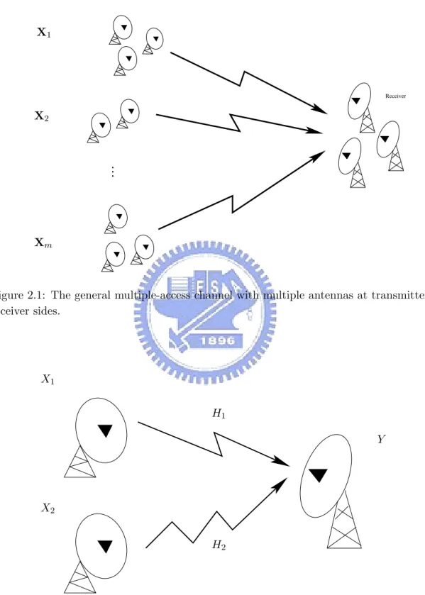
2.1 The general multiple-access channel with multiple antennas at transmitter

and receiver sides. . . 7

2.2 The two-user SISO MAC. . . 7

4.3 The plot of ξ_{7→ log(ξ) − Ei(−ξ) for ξ from 0 to 2.5. . . 14}

4.4 The plot of ξ_{7→ log(ξ) − Ei(−ξ) for ξ from 0 to 10. . . 14}

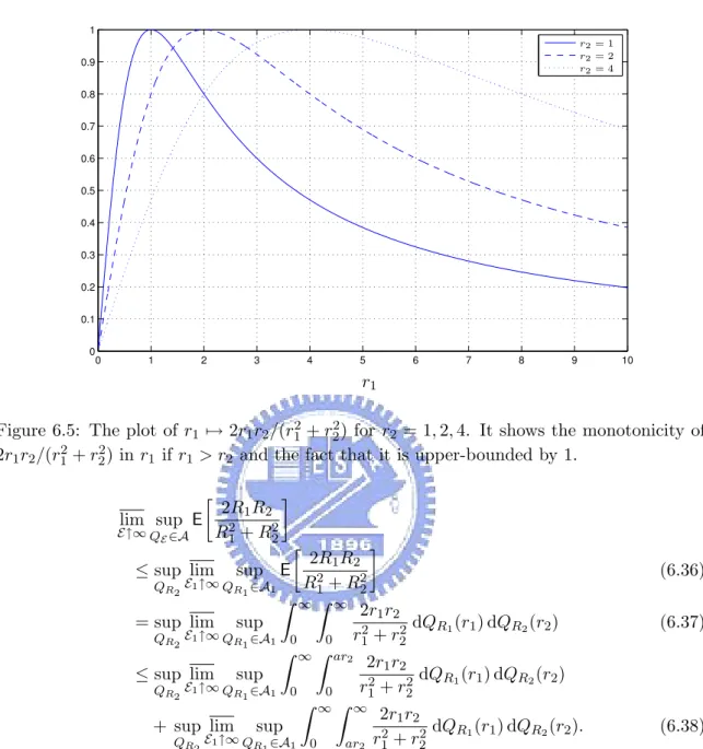
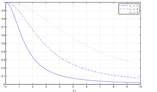
6.5 The plot of r1 7→ 2r1r2/(r21+ r22) for r2 = 1, 2, 4. It shows the monotonicity of 2r1r2/(r21+ r22) in r1 if r1 > r2 and the fact that it is upper-bounded by 1. 23 6.6 The plot of r1 7→ 2r2i/(r12+ 2r2i) for ri = 1, 2, 4. It shows the monotonicity of 2r2_i/(r₁2+ 2r_i2) in r1 and the fact that it is upper-bounded by 1. . . 29

Introduction Chapter 1

Chapter 1

Introduction

Wireless communication channels encounter additive Gaussian noise and a phenomenon called fading. The fading phenomenon impacts the signal amplitude (often destructively) and is usually modeled as a multiplicative noise. Due to this multiplicative noise, it is much more difficult to design a good communication system for such channels, and hence fading is a hot research topic. Usually channels with this fading phenomenon are called fading channels.

In this thesis we investigate the multiple-access fading channel. We restrict ourselves to the special case of Rician fading. This means that the multiplicative noise process is Gaussian distributed and that there is a line-of-sight path between the transmitter and the receiver.

Multiple-access indicates that several users utilize the channel at the same time. These users are assumed to be statistically independent, which distinguishes the multiple-user channel from the channel with a single user having multiple antennas. Common examples of the multiple-access channel (MAC) are a group of mobile phones communicating with a base station or a satellite receiver with several ground stations.

The work in this thesis focuses on the capacity analysis of the multiple-access fading channel. The concept of channel capacity was initially introduced in Shannon’s famous landmark paper “A Mathematical Theory of Communication” [1]. In this paper, Shannon proved that for every communication channel there exists a theoretically maximum rate — denoted capacity—that can be transmitted reliably, i.e., for every transmission rate below capacity the probability of making a decision error can be as small as one wishes. Therefore, the capacity is fundamental for the understanding of the channel and also for the judgment of efficiency for a designed system on a channel. However, capacity is defined in a single-user system. To generalize it to the multiple-single-user situation, we consider the theoretically maximum possible sum rate of all users. To be specific, we call this maximum possible sum rate the sum-rate capacity, but simply use capacity exchangeably in both cases.

Though many systems and techniques have been developed for the wireless communica-tion channel, the channel capacity of a general fading channel is not yet known. Researchers have been trying to solve this problem via various approaches. One common approach is to

Chapter 1

analyze the channel based on the assumption that the receiver has perfect knowledge of the channel state by estimating the channel state from training sequences. However, we cannot ignore the bandwidth kept for these training sequences. Furthermore, we can never measure the channel state perfectly even with a large amount of training data.

Another approach is to utilize joint estimation and detection: here we estimate the chan-nel state by the received information data. No assumption of a particular estimation scheme is then required. The only assumption is that both the transmitter and the receiver know the channel characteristics (but not the realizations!). The capacity under this approach of analysis is known as the noncoherent capacity.

However, no exact expression for the noncoherent capacity of a fading channel is known so far. As a function of the signal-to-noise ratio (SNR), the noncoherent capacity is only understood at asymptotic high and low SNR. Lapidoth and Moser have derived in [2] [3] [4] the asymptotic high-SNR capacity of general single-user fading channels. The asymptotic low-SNR capacity of fading channel has also been derived in [5]. In this work we extend the result of the high-SNR asymptotic capacity to the multiple-access channel.

The evaluation of noncoherent capacity involves an optimization problem. To derive the exact expression either analytically or numerically is very difficult. One promising approach is to derive upper and lower bounds to the capacity and try to make them close. Based on [6], we know natural lower and upper bounds from the single-user single-input single-out (SISO) channel and the multiple-input single-out (MISO) channel. We also know that the upper bound from the MISO channel is loose. In addition, a known upper bound is the duality-based upper bound. This duality-duality-based upper bound comes from a successful technique [7], [3] utilizing the dual expression of the channel capacity where the maximization (of mutual information) over distributions on the channel input alphabet is replaced with a minimization (of average relative entropy) over distributions on the channel output alphabet. The main contributions in this thesis are as follows. First we generalize the concept of input distributions that escape to infinity to the multiple-user case. The rough idea of escaping to infinity is that for input distributions, it is not favorable to use finite-cost input symbols whenever the cost constraint is loosened completely. Secondly, relying on this concept, we obtain the asymptotic capacity in both the two-user and general multiple-user case.

The structure of this thesis is as follows. In the remainder of this chapter we will briefly describe our notation. Next we will give a setup of the channel model in Chapter 2. The subsequent Chapter 3 gives some mathematical preliminaries about the fading number and input distributions that escape to infinity. In Chapter 4 we review the previous results as the fundamental basis of this thesis. The main result and its derivation are shown in Chapter 5 and Chapter 6, respectively. Some interesting observations not used in the proof of the main result are provided in Chapter 7, and at last we give a conclusion in Chapter 8. For random quantities we use uppercase letters such as X to denote scalar random variables and for their realizations we use lowercase letters like x. For random vectors we use bold-face capitals, e.g., X and bold lower-case letters for their realization, e.g., x. Constant matrices are denoted by upper-case letters but of a special font, e.g., H. For

Chapter 1

random matrices we yet use another font, e.g., H. Scalars are typically denoted using Greek letters or lower-case Roman letters.

Some exceptions that are widely used and therefore kept in their customary shape are: • h(·) denotes the differential entropy.

• I(·; ·) denotes the mutual information functional.

Moreover, we use the capitals Q and W as the input probability distribution and the channel law (distribution of the channel output conditioned on the channel input), and C exchange-ably for the single-user capacity and the multiple-user sum-rate capacity. The energy per symbol is denoted by _{E, and the signal-to-noise ratio SNR is denoted by snr. Also note} that we use log(_{·) to denote the natural logarithmic function.}

Channel Model Chapter 2

Chapter 2

Channel Model

In this chapter, we will introduce the channel model of the multiple-access Rician fading channel. In Section 2.1, we give the mathematical formula and some assumptions of this multiple-access channel, but restrict ourselves only to the memoryless case. In Section 2.2, we will describe the special cases of the multiple-access channel when the users in the transmitter side and the receiver use one antenna only.

2.1

The General Channel Model

In our analysis, we consider the noncoherent channel in the sense that both the transmitter and the receiver do not know the channel state realization, but only have knowledge about the channel characteristics, e.g., the distribution of the channel state.

We restrict ourselves to the memoryless case in our work. Distributions of the input and the channel are IID at every time step. Therefore, we will drop the time index.

We consider a channel as illustrated in Figure 2.1 with m users each having ni transmit

antennas for i = 1, . . . , m. The total number of transmit antennas is then

m

X

i=1

ni= nT. (2.1)

We then assume one receiver with nR receive antennas whose output Y∈ CnR is given by

Y= Hx + Z. (2.2)

Here x_{∈ C}nT _{denotes the input vector consisting of m subvectors of length n}

i for each user;

the random matrix H _{∈ C}nR×nT denotes the fading matrix; the random vector Z ∈ CnR

denotes the additive noise vector.

We assume the fading H and the additive noise Z are independent and of a joint law that does not depend on the channel input x. The different users are assumed to have access to a common clock, resulting in the output at a discrete time. Note that different users are

2.2 The Simplified Channel Model Chapter 2

not allowed to cooperate, i.e., for the input vector

X=    X1 .. . Xm    (2.3)

the subvectors Xi∈ Cni denoting the input vectors of each user are statistically independent

Xi⊥ X⊥ j, ∀ i 6= j. (2.4)

We assume that the random vector Z is a spatially white, zero-mean, circularly symmetric, complex Gaussian random vector, i.e., Z_{∼ N}C

¡

0, σ2I¢ _{for some σ}2 _{> 0. Here I denotes the} identity matrix.

As for the fading matrix H, in general it can be of any distribution. In this thesis, we restrict ourselves to the Rician fading case, i.e., every component Hi,j in the fading matrix

is given by Hi,j ∼ NC ¡ di,j, σi,j2 ¢ . (2.5) where di,j ∈ C represent the line-of-sight components and σi,j2 denotes the variance of each

component for i = 1, . . . , nR and j = 1, . . . , nT.

As for the input, two different constraints are used: a peak-power constraint or an average-power constraint. We use E to denote the maximum allowed total instantaneous power in the former case, and to denote the allowed total average power in the latter case. For both cases we get

snr_, E

σ2. (2.6)

Note that the total power still must be split and distributed among all users. The peak-power constraint is

kXk2 ≤ E, almost surely. (2.7) The average-power constraint is given by

E£_kXk2¤_{≤ E. (2.8)}

2.2

The Simplified Channel Model

For simplicity, we first assume that each user and the receiver use only one antenna, i.e., n1 = n2 = · · · = nm = 1, such that nT = m, and nR = 1. This reduces (2.2) to the

multiple-access SISO case: the channel output Y _{∈ C is:}

Y = HT_{x+ Z (2.9)}

= dT_{x+ ˜H}T_{x+ Z (2.10)}

2.2 The Simplified Channel Model Chapter 2

Here x∈ Cm _{denotes the input vector. The components x}

i in x are the input of each user.

H denotes the fading vector where each component is a random variable representing the channel state for each user. By the assumption of Rician fading we have

˜

Hi+ di = Hi∼ NC(di, 1) , i = 1, . . . , m, (2.12)

i.e., ˜Hi are zero-mean, circularly symmetric, complex Gaussian random variables with

vari-ance 1. Moreover, the channels are assumed to be independent

Hi⊥ H⊥ j, i, j = 1, . . . , m, i6= j, (2.13)

and Z _{∼ N}C

¡

0, σ2¢ denotes additive, zero-mean, circularly symmetric Gaussian noise. A special simplified case is the two-user multiple-access Rician fading channel as shown in Figure 2.2. We use this most simplified case at the beginning of our analysis. In this case we assume there are only two users, i.e., m = 2, and n1= n2 = 1 so that nT= 2, and

nR= 1. The channel output can be written as

Y = H1x1+ H2x2+ Z (2.14)

= d1x1+ ˜H1x1+ d2x2+ ˜H2x2+ Z, (2.15)

where Hi and Z are as described before. Also recall that the two users are not allowed to

cooperate, i.e.,

X1⊥ X⊥ 2 (2.16)

is required.

Given X1 = x1 and X2 = x2 the channel output is Gaussian distributed:

2.2 The Simplified Channel Model Chapter 2 Receiver X1 X2 Xm

...

Figure 2.1: The general multiple-access channel with multiple antennas at transmitter and receiver sides. X1 X2 Y H1 H2

Mathematical Preliminaries Chapter 3

Chapter 3

Mathematical Preliminaries

In this chapter we review some important concepts mainly related to the analysis of the single-user memoryless case. The channel model considered is (2.2). In Section 3.1 we review the channel capacity and make a further generalization to the maximum possible sum rate of multiple users. In Section 3.2 we introduce the fading number. In Section 3.3 we provide the concept of input distributions that escape to infinity and a lemma which shows that under some conditions the input distribution must escape to infinity. The concepts mentioned in this chapter are strongly based on [2] and [3].

3.1

The Channel Capacity

In this section we first review the definition of channel capacity provided by Shannon in [1]. Further we give the definition of the maximum possible sum rate of the multiple-access channel; it is basically identical to the channel capacity, but takes multiple users into consideration.

Recall that in a discrete memoryless channel (DMC), the channel capacity is defined as

C_{, max}

QX

I(X; Y ) (3.1)

where the maximization is taken over all possible input distributions QX(·). When the

concept is generalized to the continuous case, i.e., the input and output take values in continuous alphabet, a power constraint must be taken into consideration: for the peak power constraint (2.7) C_{, max} QX |X|2 ≤E I(X; Y ), (3.2)

or for the average power constraint (2.8)

C_{, max}

QX

E[X2

]≤E

3.2 The Fading Number Chapter 3

where the maximization is taken over all the input distributions satisfying the constraint. In the generalization to the memoryless multiple-user channel, we use C to denote the maximum possible sum rate. The (sum-rate) capacity of the channel (2.2) is given by

C_{= sup}

QX

I(X; Y) (3.4)

where the supremum is taken over the set of all probability distributions on X for which the m subvectors are independent and which satisfy the power constraint, i.e.,

kXk2≤ E, almost surely (3.5) for a peak-power constraint, or

E£_kXk2¤_{≤ E (3.6)} for an average-power constraint.

3.2

The Fading Number

In the asymptotic analysis of channel capacity at high SNR, it has been shown in [2],[3] that at high SNR capacity grows only double-logarithmically in the SNR. This means that at high power these channels become extremely power-inefficient because we have to square the SNR to get an additional bit improvement in capacity. Furthermore, the difference between channel capacity and log log SNR is bounded as the SNR tends to infinity, i.e.,

lim E↑∞ ½ C_{(E) − log log} E σ2 ¾ <∞. (3.7)

This bounded term is called the fading number. A precise definition of the fading number is as follows.

Definition 3.1. The fading number χ of a memoryless fading channel with fading matrix

H_{is defined as} χ(H)_{, lim} E↑∞ ½ C_{(E) − log log} E σ2 ¾ . (3.8)

Whenever the limit in (3.8) exists and χ is finite, the expression of capacity is

C_{(E) = log log} E

σ2 + χ + o(1) (3.9)

where o(1) denote terms that tend to zero as the SNR tends to infinity. Thus, at high SNR the channel capacity of a fading channel can be approximated by

C_{(E) ≈ log log} E

σ2 + χ. (3.10)

Hence we can say that the fading number is the second term in the asymptotic expression of the channel capacity at high SNR. Note that the approximation of capacity in (3.10) is

3.3 Escaping to Infinity Chapter 3

not always valid. In the low-SNR to medium-SNR regime, the capacity is dominated by the o(1) term that cannot be neglected in that regime. In the analysis of the asymptotic capacity, however, we are only concerned with the high-SNR regime and in particular when the SNR tends to infinity. Thus, we usually use the approximation of (3.10) instead of the intractable exact expression. Furthermore, we can even only consider the fading number because the first term of the capacity is always the same.

The fading number also plays a role as a qualitative criterion for the communication system. Since in the high-SNR regime the capacity is extremely power-inefficient, we should avoid transmission in this severe regime. The fading number can provide a threshold of how high the rate can be before entering the high-SNR regime, i.e., the fading number can provide a certain threshold snr0 such that once the available SNR is above snr0, we are in

the log log snr dominated regime, and should not stick on this system. Instead we should use other schemes, e.g., use more antennas in order to reach a higher transmission rate.

3.3

Escaping to Infinity

A sequence of input distributions parameterized by the allowed cost (in our case the cost of fading channels is the available power or the SNR, respectively) is said to escape to infinity if it assigns to every fixed compact set a probability that tends to zero as the allowed cost tends to infinity. In other words this means that in the limit—when the allowed cost tends to infinity—such a distribution does not use finite-cost symbols.

We give the definition of escaping to infinity for the fading channel under consideration in this thesis; the definition for general channels can be found in [2], [3].

Definition 3.2. Let {QE}E≥0 be a family of input distributions for the memoryless fading

channel (2.2), where this family is parameterized by the available average power _{E such that}

E_QE£_kXk2¤_{≤ E, E ≥ 0. (3.11)}

We say that the input distributions {QE}E≥0 escape to infinity if for every E0

lim

E↑∞QE

¡

kXk2≤ E0¢= 0. (3.12)

This notion is of importance because the asymptotic capacity of the fading channels can only be achieved by input distributions that escape to infinity. As a matter of fact one can show that to achieve a mutual information of only identical asymptotic growth rate as the capacity, the input distribution must escape to infinity. The following lemma describes this fact.

Lemma 3.3. Assume a single-user memoryless multiple-input multiple-output (MIMO)

fad-ing channel as given in (2.2) and let W (_{·|·) denote the corresponding conditional channel}

law. Let _{QE}E≥0 be a family of input distributions satisfying the power constraint (3.11)

and the condition

lim

E↑∞

I(QE, W )

3.3 Escaping to Infinity Chapter 3

Then {QE}E≥0 escapes to infinity.

Proof. A proof can be found in [2], [3].

From the engineering point of view, this concept matches the intuition: as the available power tends to infinity, the input should utilize the resource (available power) completely, therefore any fixed symbol is not used in the limit.

Remark 3.4. When computing the bounds of the fading number (which is part of the

capac-ity in the limit when _{E tends to infinity), we can therefore assume that for any fixed value}

E0

Previous Results Chapter 4

Chapter 4

Previous Results

In this chapter we review some known results of the simplified two-user SISO case (2.14) and (2.15). In Section 4.1 we show that the sum rate of the two users is bounded between the single-user MISO capacity and the single-user SISO capacity. In Section 4.2 we review a known bound of the sum-rate capacity in our case. The content in this chapter is mainly based on [6].

4.1

Natural Upper and Lower Bounds

We consider the channel model of a two-user SISO fading channel as in (2.14) and (2.15). Note that the difference between the MAC and the MISO fading channel with two transmit antennas and one receive antenna is that in the latter both transmit antennas can cooperate, while in the former they are assumed to be independent. Hence, it immediately follows from this that the MAC sum-rate capacity can be upper-bounded by the MISO capacity:

C_{MAC(E) ≤ CMISO(E). (4.1)} On the other hand, the sum rate cannot be smaller than the single-user rate that can be achieved if the weaker of the two users is switched off, i.e.,

C_{MAC(E) ≥ max}

i=1,2

C_{SISO,i(E). (4.2)} Based on (4.1), (4.2) and (3.8), we define the MAC fading number by

χMAC, lim E↑∞

½

C_{MAC(E) − log log} E σ2

¾

. (4.3)

From [3] we know that

χMISO= log ¡ |d1|2+|d2|2 ¢ − Ei¡−|d1|2− |d2|2 ¢ − 1 (4.4) where Ei(_{−·) is the exponential integral function defined as}

Ei(_{−ξ) , −} Z ∞

ξ

e−t

4.2 An Upper Bound on the Sum-Rate Capacity and Fading NumberChapter 4

Therefore, from (4.1) we obtain

χMAC≤ χMISO= log¡|d1|2+|d2|2¢− Ei¡−|d1|2− |d2|2¢− 1. (4.6)

On the other hand from (4.2) χMAC≥ max

i=1,2χSISO,i = maxi

© log¡|di|2 ¢ − Ei¡−|di|2 ¢ − 1ª. (4.7)

Using the monotonicity of ξ _{7→ log(ξ) − Ei(−ξ) as shown in Figure 4.3 and Figure 4.4 and} comparing (4.6) and (4.7), the sum-rate capacity of two-user MAC can be written as a similar expression

χMAC= log¡d2MAC

¢

− Ei¡−d2MAC

¢

− 1 (4.8) where dMAC is a nonnegative real number satisfying

max{|d1|, |d2|} ≤ dMAC≤

p

|d1|2+|d2|2. (4.9)

Note that the difference between χMAC, χMISO, and χSISO is the parameter of the function

log(·) − Ei(−·). Thus, we can investigate dMAC instead of the whole fading number.

Furthermore, from [8] we actually know that dMAC<

p

|d1|2+|d2|2 (4.10)

with strict inequality.

4.2

An Upper Bound on the Sum-Rate Capacity and Fading

Number

Since the multiple-access channel is quite similar to the MISO channel, we review an upper bound on the MISO capacity. This upper bound comes from the dual expression of the mu-tual information by choosing the output distribution as a generalized Gamma distribution. A detailed proof of this lemma can be found in [2] and [3].

Lemma 4.1. Consider a memoryless MISO fading channel with input x∈ CnT _{and output}

Y ∈ C such that

Y = HT_{x+ Z. (4.11)}

Then the mutual information between input and output of the channel is upper-bounded as follows:

I(X; Y )≤ −h(Y |X) + log π + α log β + log Γ µ α,ν β ¶ + (1_{− α)E}£log¡_{|Y |}2+ ν¢¤+ 1 βE £ |Y |2¤+ ν β (4.12)

where α, β > 0 and ν_{≥ 0 are parameters that can be chosen freely, but must not depend on}

4.2 An Upper Bound on the Sum-Rate Capacity and Fading NumberChapter 4 0 0.5 1 1.5 2 2.5 −0.6 −0.4 −0.2 0 0.2 0.4 0.6 0.8 1 ξ log(ξ)_{− Ei(−ξ)}

Figure 4.3: The plot of ξ 7→ log(ξ) − Ei(−ξ) for ξ from 0 to 2.5.

0 1 2 3 4 5 6 7 8 9 10 −1 −0.5 0 0.5 1 1.5 2 2.5 ξ log(ξ)− Ei(−ξ)

4.2 An Upper Bound on the Sum-Rate Capacity and Fading NumberChapter 4

Applying Lemma 4.1 to the Rician fading channel (2.15), we have:

I(X1, X2; Y )≤ −h(Y |X1, X2) + log π + α log β + log Γ

µ α,ν β ¶ + (1− α)E£log¡|Y |2+ ν¢¤+ 1 βE £ |Y |2¤+ ν β. (4.13) Using the fact in (2.17) that given X1 = x1 and X2 = x2, Y is Gaussian distributed, and

choosing the parameters α, β and ν appropriately, (4.13) can be further simplified to obtain an upper bound on the fading number of the MAC:

Theorem 4.2. The fading number of a two-user Rician fading MAC as defined in (2.14) and under the average-power constraint (2.8) is upper-bounded as follows:

χMAC ≤ lim E↑∞_QX1sup_·QX2 ( log E· |d1X1+ d2X2| 2 |X1|2+|X2|2 ¸ − Ei µ −E· |d1X1+ d2X2| 2 |X1|2+|X2|2 ¸¶ − 1 ) . (4.14)

Proof. The theorem is a special case of the Proposition 6.1. The proof can be found in

Appendix A or in [6].

Note that ξ 7→ log(ξ) − Ei(−ξ) is monotonically increasing, thus according to Theo-rem 4.2, the parameter dMAC defined in (4.8) is upper-bounded as follows:

d2_{MAC ≤} sup QX1·QX2 E· |d1X1+ d2X2| 2 |X1|2+|X2|2 ¸ . (4.15)

Main Result Chapter 5

Chapter 5

Main Result

In this chapter, the exact MAC fading number is provided. In Section 5.1 we extend the notion of escaping to infinity to multiple users. In Section 5.2, we will show the two-user SISO MAC sum-rate fading number. In Section 5.3, we generalize to the m-user SISO MAC and provide its sum-rate fading number; and in Section 5.4 we discuss the power constraints.

5.1

Generalization of Escaping to Infinity to Multiple Users

The following proposition is a generalization of Lemma 3.3.

Proposition 5.1. Let_{QE}E≥0be a family of joint input distributions of the multiple-access

fading channel given in (2.2), where the family is parameterized by the available average

power _{E such that}

E_QE£_kXk2¤_{≤ E, E ≥ 0. (5.1)}

Let W (_{·|·) be the channel law, and {Q}E} be such that

lim

E↑∞

I(QE, W )

log logE = 1. (5.2)

Then at least one user’s input distribution must escape to infinity, i.e., for any_E0 > 0,

lim E↑∞QE Ã_m [ i=1 ½ ° °Xi ° °2 ≥ E0 m ¾! = 1. (5.3)

5.2

The Fading Number of The Two-User SISO MAC

Theorem 5.2. Assume a two-user SISO Rician fading MAC channel as defined in (2.15). Then the sum-rate fading number is given by

χMAC = log¡d2MAC

¢

− Ei¡−d2MAC

¢

5.3 The Fading Number of General SISO MAC Chapter 5

where

dMAC = max©|d1|, |d2|ª. (5.5)

This sum-rate MAC fading number holds in both cases when the peak-power constraint (2.7) or the average-power constraint (2.8) is considered.

This shows that the lower bound in (4.2) is tight. Note that if the magnitude of the line-of-sight component of one user is strictly smaller than of the other user, then this sum rate can only be achieved if the user with the weaker_|di| is switched off. If both line-of-sight

components have identical magnitudes, then the sum rate can be achieved by time-sharing. Remark 5.3. Recall that in [6, Lemma 17] the distribution taking only two symbols causes an opposite result: the natural upper bound to the MAC fading given in (4.6) can be achieved by the binary input distribution. Relying on Proposition 5.1, any input distribution that takes value in finite-cost symbols is excluded from being the capacity achieving distribution of the multiple-access fading channel.

5.3

The Fading Number of General SISO MAC

Theorem 5.4. Assume a SISO Rician fading multiple-access channel as defined in (2.9). Then the sum-rate fading number is given by

χMAC = log ¡ d2_MAC¢− Ei¡−d2MAC ¢ − 1 (5.6) where dMAC = max©|d1|, |d2|, . . . , |dm|ª. (5.7)

This sum-rate MAC fading number holds in both cases when the peak-power constraint (2.7) or the average-power constraint (2.8) is considered.

The result for the general m users is similar to the two-user case. The SISO MAC fading number is exactly the same as the single-user SISO fading number. To achieve the fading number, the input should only allow the user with the largest line-of-sight component to transmit, and switch off all users with weaker _|di|. If several users encounter channels with

a line-of-sight component of maximum magnitude, time-sharing among these users can be used to achieve the fading number.

5.4

Discussion on Power Constraints

In our channel model, we consider the average total power constraint of all users, and even allow power allocation among the users, i.e., the users can share the total power and the power constraints for individual user are loosened.

5.4 Discussion on Power Constraints Chapter 5

However, note that both Theorem 5.2 and Theorem 5.4 continue to hold even if we do not allow power optimization over the users, i.e., if we constrain the inputs to satisfy

|Xi|2 ≤ E

m, almost surely, ∀i. (5.8) Because both the looser and the more stringent cases lead to the same result, the re-sults hold implicitly for other cases in between these two cases with respect to the power constraints.

Derivation of Results Chapter 6

Chapter 6

Derivation of Results

In this chapter, the derivations of the results shown in Chapter 5 are provided. In Section 6.1, the generalization of the concept of escaping to infinity to multiple users is mainly based on the proof of the single-user case in [3, Theorem 2.6]. In Section 6.2 and Section 6.3, the SISO MAC sum-rate fading number of the two-user and m-user cases are derived strongly relying on the concepts provided in Section 3.3 and Section 5.1.

6.1

Derivation of Proposition 5.1

From (4.1) and (4.2) we know that the asymptotic behavior of CMAC(E) is equivalent to

the behavior of the single-user fading channel capacity shown in (3.9), i.e., we can write C_{MAC(E) = log log} E

σ2 + χMAC+ o(1). (6.1)

Note that this expression is also valid in the general m-user case. So we have the following:

lim

E↑∞

C_MAC(E)

log log_E = 1. (6.2) Moreover note that

lim E↑∞ ( sup µ∈(0,µ0] µ log logE_µ log logE ) < 1, _{∀ 0 < µ}0< 1. (6.3)

Fix some_E0> 0 and let

E ,            1 if m [ i=1 ½ kXik2≥ E0 m ¾ , 0 if m \ i=1 ½ kXik2< E0 m ¾ . (6.4) and µ_{, Pr[E = 1] .} (6.5)

6.1 Derivation of Proposition 5.1 Chapter 6 Then I(X; Y) = I (X, E; Y) (6.6) = I(E; Y) + I (X; Y_{| E)} (6.7) = I(E; Y) + I (X; Y_{| E = 0) Pr[E = 0]} + I (X; Y| E = 1) Pr[E = 1] (6.8) ≤ log 2 + I (X; Y | E = 0) + µI (X; Y | E = 1) (6.9) ≤ log 2 + CMAC(E0) + µCMACµ E

µ ¶

, (6.10)

where the first inequality follows because E is a binary random variable and because Pr[E = 0]_{≤ 1; the subsequent inequality follows from that conditional on E = 0,}

E£_kXk2¯¯E = 0¤<E₀, (6.11) and E£_kXk2¤_{= µE}£_kXk2¯¯ E = 1¤+ (1− µ)E£kXk2¯¯ E = 0¤ | {z } ≥0 (6.12) ≥ µE£kXk2¯¯ E = 1¤ (6.13) from which follows that

E£_kXk2¯¯ E = 1¤≤ E £ kXk2¤ µ ≤ E µ. (6.14) To show µ _{↑ 1, let E}n be a sequence with En ↑ ∞. Let {QEn} be a family of joint input

distributions on the MAC channel (2.2) such that

lim n↑∞ I(QEn, W ) log logEn = 1 (6.15) and define µn, QEn Ã_m [ i=1 ½ ° °Xi°°2 ≥ E0 m ¾! (6.16)

By contradiction, assume µn→ µ∗ < 1. Then∃ µ0 < 1 such that

µn< µ0, n sufficiently large. (6.17) From (6.10) we have I(X; Y) log logEn | {z } →1 ≤ log 2 + CMAC(E0) log logEn | {z } →0 + C_MAC³En µn ´ log logEn µn | {z } →1 ·µnlog log En µn log logEn (6.18)

6.2 Derivation of Theorem 5.2 Chapter 6

Here the limiting behavior of the LHS follows from (6.15); the first term on the RHS tends to zero because CMAC(E0) <∞; the second term on the RHS

C_MAC³En µn ´ log logEn µn → 1 (6.19)

follows becauseEn↑ ∞ implies En/µn↑ ∞ and because of (6.2). So, when n ↑ ∞ we obtain

the following contradiction

1_{≤ lim} n↑∞ µnlog logE_µn_n log log_En (6.20) ≤ lim E↑∞ ( sup µ∈(0,µ0] µ log logE_µ log log_E ) (6.21) < 1, (6.22)

where the first inequality follows from (6.18); the second inequality follows from (6.17), and the last inequality follows from (6.3).

6.2

Derivation of Theorem 5.2

The proof of Theorem 5.2 consists of two parts. The first part is given already in (4.9). There it is shown that max_{|d1|, |d2|} is a lower bound to dMAC. Note that this lower bound

can be achieved by using an input that satisfies the peak-power constraint.

The second part will be to prove that max_{|d1|, |d2|} is also an upper bound. We

will prove this under the assumption of an average-power constraint. Since a peak-power constraint is more stringent than an average-power constraint, the result follows.

The proof of this upper bound relies strongly on the Proposition 5.1. From that the supremum in (4.14) should be replaced by the supremum taken over all joint distributions such that at least one user’s input distribution escapes to infinity. So (4.14) becomes

χMAC ≤ lim E↑∞_Qsup_E∈A

( log E· |d1X1+ d2X2| 2 |X1|2+|X2|2 ¸ − Ei µ −E· |d1X1+ d2X2| 2 |X1|2+|X2|2 ¸¶ − 1 ) . (6.23)

Here we defineA to be the set of joint input distributions such that X1⊥ X⊥ 2 and the input

distribution of at least one user escapes to infinity when the available power E tends to infinity, i.e., A , ½ QX1,X2 ¯ ¯ ¯ ¯X1⊥ X⊥ 2, E↑∞limQE ¡© |X1|2≥ E0/2ª∪©|X2|2≥ E0/2ª¢= 1

for any fixed_E0> 0

¾

6.2 Derivation of Theorem 5.2 Chapter 6

Following the same argument as given after Theorem 4.2, we note that since ξ 7→ log(ξ) − Ei(_{−ξ) is monotonically increasing, finding the MAC fading number is reduced to finding} dMAC which is upper-bounded by

d2_{MAC≤ sup} QE∈A E· |d1X1+ d2X2| 2 |X1|2+|X2|2 ¸ . (6.25) 6.2.1 Symmetric Case

In the following we will first prove the theorem for the special case when d1 = d2= d. The

proof for general d1, d2 will be provided later.

Continuing from (6.25) and writing Xi= RieiΦi, we have

d2_{MAC≤ sup} QE∈A E· |dX1+ dX2| 2 |X1|2+|X2|2 ¸ (6.26) = sup QE∈A E· |d| 2_|X 1+ X2|2 |X1|2+|X2|2 ¸ (6.27) = sup QE∈A E · |d|2 µ 1 +2|X1||X2| cos(Φ1− Φ2) |X1|2+|X2|2 ¶¸ (6.28) =|d|2 à 1 + sup QE∈A E· 2|X1||X2| cos(Φ1− Φ2) |X1|2+|X2|2 ¸! (6.29) ≤ |d|2 à 1 + sup QE∈A E· 2R1R2 R2₁+ R2₂ ¸! , (6.30)

where in the last inequality we upper-bounded cos(Φ1 − Φ2) ≤ 1. The result now follows

once we can show that

lim

E↑∞_Qsup_E∈A

E· 2R1R2 R2

1+ R22

¸

= 0. (6.31)

To that goal let

E£_|X1|2¤_{≤ E1 (6.32)} E£_|X2|2¤_{≤ E2 (6.33)} where

E1+E2=E. (6.34)

Note that from Proposition 5.1 we know that if _{E ↑ ∞ then E}1 ↑ ∞ or E2 ↑ ∞ or both.

Without loss of generality assume thatE1↑ ∞. Note further that

2r1r2

r2 1+ r22

≤ 1 (6.35)

and that r1 7→ 2r1r2/(r12 + r22) is monotonically decreasing in r1 if r1 > r2 as shown in

6.2 Derivation of Theorem 5.2 Chapter 6 0 1 2 3 4 5 6 7 8 9 10 0 0.1 0.2 0.3 0.4 0.5 0.6 0.7 0.8 0.9 1 r₂= 1 r₂= 2 r₂= 4 r1

Figure 6.5: The plot of r1 7→ 2r1r2/(r21 + r22) for r2 = 1, 2, 4. It shows the monotonicity of

2r1r2/(r21+ r22) in r1 if r1> r2 and the fact that it is upper-bounded by 1.

lim

E↑∞_QsupE∈A

E· 2R1R2 R2₁+ R2₂ ¸ ≤ sup QR2 lim E1↑∞ sup QR1∈A1 E· 2R1R2 R2 1+ R22 ¸ (6.36) = sup QR2 lim E1↑∞ sup QR1∈A1 Z ∞ 0 Z ∞ 0 2r1r2 r2₁+ r2₂ dQR1(r1) dQR2(r2) (6.37) ≤ sup QR2 lim E1↑∞ sup QR1∈A1 Z ∞ 0 Z ar2 0 2r1r2 r2 1+ r22 dQR1(r1) dQR2(r2) + sup QR2 lim E1↑∞ sup QR1∈A1 Z ∞ 0 Z ∞ ar2 2r1r2 r2₁+ r2₂ dQR1(r1) dQR2(r2). (6.38)

Here in the first inequality we define _A1 as the set of all input distributions of the first

user that escape to infinity, we use that from _{E ↑ ∞ we know that E}1 ↑ ∞ and take the

supremum over all QR2 without any constraint on the average power and no dependence

on QR1. The last inequality then follows from splitting the integration into two parts and

from the property that the supremum of a sum is always upper-bounded by the sum of the suprema.

Next, let’s look at the first term in (6.38):

lim E1↑∞ sup QR1∈A1 Z ∞ 0 Z ar2 0 2r1r2 r₁2+ r2₂ | {z } ≤1 dQR1(r1) dQR2(r2)

6.2 Derivation of Theorem 5.2 Chapter 6 ≤ lim E1↑∞ sup QR1∈A1 Z ∞ 0 Z ar2 0 dQR1(r1) dQR2(r2) (6.39) ≤ lim E1↑∞ Z ∞ 0 sup QR1∈A1 Z ar2 0 dQR1(r1) dQR2(r2) (6.40) = Z ∞ 0 lim E1↑∞ sup QR1∈A1 Z ar2 0 dQR1(r1) dQR2(r2) (6.41) = Z ∞ 0 0 dQR2(r2) (6.42) = 0. (6.43) Here, (6.42) follows because QR1 escapes to infinity; and in (6.41) we exchange the limit

and the integration which can be justified as follows: let

gE1(r2), sup QR1∈A1 Z ar2 0 dQR1(r1) (6.44) ≤ sup QR1∈A1 Z ∞ 0 dQR1(r1) (6.45) = 1_{, g}upper(r2) (6.46)

Then note that

Z ∞ 0 gupper(r2) dQR2(r2) = Z ∞ 0 dQR2(r2) = 1, (6.47)

i.e., gupper(·) is independent of E1 and integrable. Thus, by the Dominated Convergence

Theorem (DCT) [10, Chapter 14] we are allowed to swap limit and integration. Continuing with (6.38) we get:

lim

E↑∞_Qsup_E∈A

E· 2R1R2 R₁2+ R2₂ ¸ ≤ sup QR2 lim E1↑∞ sup QR1∈A1 Z ∞ 0 Z ∞ ar2 2r1r2 r2 1+ r22 dQR1(r1) dQR2(r2) (6.48) ≤ sup QR2 lim E1↑∞ sup QR1∈A1 Z ∞ 0 Z ∞ ar2 2(ar2)r2 (ar2)2+ r22 dQR1(r1) dQR2(r2) (6.49) = sup QR2 lim E1↑∞ sup QR1∈A1 Z ∞ 0 Z ∞ ar2 2a a2_{+ 1}dQR1(r1) dQR2(r2) (6.50) ≤ sup QR2 lim E1↑∞ sup QR1∈A1 Z ∞ 0 Z ∞ 0 2a a2_{+ 1}dQR1(r1) dQR2(r2) (6.51) = 2a a2_{+ 1}sup QR2 lim E1↑∞ sup QR1∈A1 Z ∞ 0 Z ∞ 0 dQR1(r1) dQR2(r2) (6.52) = 2a a2_{+ 1} < ǫ if a large enough. (6.53)

Here (6.49) follows because r17→ 2r1r2/(r12+ r22) is monotonically decreasing in r1 if r1 > r2.

6.2 Derivation of Theorem 5.2 Chapter 6

6.2.2 Asymmetric Case

Next we will investigate the general d1, d2. Assuming that |d1| > |d2| without loss of

generality, we again start with (6.25) and write di =|di|eiψi and Xi = RieiΦi.

d2_{MAC≤ sup} QE∈A E· |d1X1+ d2X2| 2 |X1|2+|X2|2 ¸ (6.54) = sup QE∈A E " |d1X1|2+|d2X2|2+ d*1X1*d2X2+ d1X1d*2X2* |X1|2+|X2|2 # (6.55) = sup QE∈A E· |d1| 2_R2 1+|d2|2R22+ 2|d1||d2|R1R2cos(Φ2+ ψ2− Φ1− ψ1) R2₁+ R2₂ ¸ (6.56) ≤ sup QE∈A E· |d1| 2_R2 1+|d2|2R22+ 2|d1||d2|R1R2 R2₁+ R₂2 ¸ (6.57) ≤ sup QE∈A E· |d1| 2_R2 1+|d2|2R22 R2 1+ R22 ¸ + sup QE∈A E· 2|d1||d2|R1R2 R2 1+ R22 ¸ . (6.58)

Here the first inequality follows from cos(Φ2 + ψ2 − Φ1 − ψ1) ≤ 1, and the subsequent

inequality follows from that the supremum of the sum is less equal to the sum of the suprema.

Let’s first look at the first term in (6.58). We define a matrix ˜D _{as a diagonal matrix} where the components on its diagonal are_|di|2, i.e.,

˜ D_{= diag}¡_|d1|2_,|d2|2¢₌ Ã |d1|2 0 0 |d2|2 ! (6.59) Note that sup QE∈A E· |d1| 2_R2 1+|d2|2R22 R2 1+ R22 ¸ ≤ sup r1,r2 |d1|2r12+|d2|2r22 r2 1+ r22 (6.60) = sup r rT_D˜_r krk2 (6.61) = λmax( ˜D) (6.62)

where in the first equality r, (r1, r2)T, and in the subsequent equality λmax( ˜D) denotes the

maximum eigenvalue of the matrix ˜D_{. Here the last equality follows from the Rayleigh-Ritz} Theorem [11, Theorem 4.2.2]. The maximum eigenvalue of ˜D_{is evidently |d1|}2_{, so we know}

sup QE∈A E· |d1| 2_R2 1+|d2|2R22 R2 1+ R22 ¸ ≤ |d1|2 (6.63)

Next, note that for the second term in (6.58)

lim

E↑∞_Qsup_E∈A

E· 2|d1||d2|R1R2 R2

1+ R22

¸

=|d1||d2| lim E↑∞_Qsup_E∈A

E· 2R1R2 R2 1+ R22 ¸ (6.64) =_|d1||d2| · 0 (6.65) = 0 (6.66)

6.3 Derivation of Theorem 5.4 Chapter 6

where (6.65) follows from (6.31). Note that (6.31) also holds for asymmetric |d1| and |d2|.

We have shown that (6.31) is true by assuming R1 escapes to infinity in Section 6.2.1; for

R2 escaping to infinity the proof is identical so we omit it.

From (6.58), (6.63) and (6.66) we obtain the following:

lim

E↑∞_Qsup_E∈A

E· |d1X1+ d2X2|

2

|X1|2+|X2|2

¸

≤ |d1|2 (6.67)

therefore our result follows for the asymmetric case.

6.3

Derivation of Theorem 5.4

In this section, we step further to general m-user SISO MAC. Our goal is to derive upper and lower bounds to dMAC. From the same argument in Section 4.1 we know that

χMAC≥ max

i=1,...,mχSISO,i = maxi=1,...,m

©

log¡|di|2¢− Ei¡−|di|2¢− 1ª. (6.68)

and hence we get

dMAC≥ max{|d1|, . . . , |dm|}. (6.69)

Once the upper bound to dMACcan be shown to be equivalent to the lower bound in (6.69),

we complete the proof of the result. Note that the lower bound (6.69) can be achieved by using an input that satisfies the peak-power constraint, while we will derive the upper bound under the average-power constraint.

Using the upper bound in (4.13) for the channel model (2.11), we can get after some steps the bound

I(X; Y )_{≤ −1 + E} · log|d1X1+· · · + dmXm| 2 |X1|2+· · · + |Xm|2 − Ei µ −|d1X1+· · · + dmXm| 2 |X1|2+· · · + |Xm|2 ¶¸ + ǫν

+ α(log β− log σ2+ γ) + log Γ µ α,β γ ¶ + 1 β ¡¡ 1 + d2_max¢E + σ2¢+ ν β (6.70) which with the right choice of the free parameters α, β, and ν leads to the following propo-sition.

Proposition 6.1. For the Rician fading MAC (2.9), an upper bound of the sum-rate fading number under the average-power constraint (2.8) is given as follows:

χMAC≤ lim E↑∞_Qsup_E∈A

( log E· |d1X1+· · · + dmXm| 2 |X1|2+· · · + |Xm|2 ¸ − Ei µ −E· |d1X1+· · · + dmXm| 2 |X1|2+· · · + |Xm|2 ¸¶ − 1 ) . (6.71)

Here we defineA to be the set of joint input distributions such that all users are independent

and at least one user’s input distribution escapes to infinity when the available power_{E tends} to infinity.

6.3 Derivation of Theorem 5.4 Chapter 6

Proof. A proof is provided in Appendix A.

Since ξ 7→ log(ξ) − Ei(−ξ) is monotonically increasing, the problem of deriving an upper bound to dMAC can be transformed to finding an upper bound of the expression:

E· |d1X1+· · · + dmXm|

2

|X1|2+· · · + |Xm|2

¸

. (6.72)

Note that (6.72) is equivalent to

E· |d1| 2_|X 1|2+· · · + |dm|2|Xm|2 |X1|2+· · · + |Xm|2 ¸ + m X j=1 m X i=1 i6=j E " did*jXiXj* |X1|2+· · · + |Xm|2 # . (6.73)

Assume _|d1| ≥ |d2| ≥ · · · ≥ |dm| without loss of generality. For the first term in (6.73), we

can upper-bound it as follows:

sup QE∈A E· |d1| 2_|X 1|2+· · · + |dm|2|Xm|2 |X1|2+· · · + |Xm|2 ¸ = sup QE∈A E· |d1| 2_R2 1+· · · + |dm|2R2m R2 1+· · · + R2m ¸ (6.74) ≤ sup r1,...,rm |d1|2r21+· · · + |dm|2r2m r₁2+· · · + r2 m (6.75) = sup r rT_D˜_r krk2 (6.76) = λmax( ˜D) (6.77) =|d1|2. (6.78) Here in (6.76) we define ˜ D_{= diag}¡_|d1|2_{, . . . ,|dm|}2¢_{. (6.79)} and r_,    r1 .. . rm    . (6.80)

In (6.77) we use Rayleigh-Ritz Theorem as in Section 6.2.2, and (6.78) follows because the maximum eigenvalue of ˜D_{is |d1|}2_.

As for the second term in (6.73), we write Xi = RieiΦi and di=|di|eiψi and get m X j=1 m X i=1 i6=j E " did*jXiXj* |X1|2+· · · + |Xm|2 # = E · 2_|d1|R1 R2 1+· · · + Rm2 ³ |d2|R2cos(Φ2+ ψ2− Φ1− ψ1) +· · · +|dm|Rmcos(Φm+ ψm− Φ1− ψ1) ´

6.3 Derivation of Theorem 5.4 Chapter 6 + 2|d2|R2 R2 1+· · · + R2m ³ |d3|R3cos(Φ3+ ψ3− Φ2− ψ2) +· · · +_|dm|Rmcos(Φm+ ψm− Φ2− ψ2) ´ + _{· · · +} 2|dm−1|Rm−1 R2₁+· · · + R2 m|d m|Rmcos(Φm+ ψm− Φm−1− ψm−1) ¸ (6.81) ≤ E " 2_|d1|R1¡|d2|R2+· · · + |dm|Rm¢ R2 1+· · · + R2m # + E " 2_|d2|R2¡|d3|R3+· · · + |dm|Rm¢ R2 1+· · · + R2m # + _{· · · + E}· 2|dm−1|Rm−1|dm|Rm R2₁+· · · + R2 m ¸ (6.82)

Assuming that QR1 escapes to infinity, we can separate (6.82) into two kinds of products as

follows E· 2|d1||di|R1Ri R2 1+· · · + Rm2 ¸ for i = 2, . . . , m, (6.83) and E· 2|di||dj|RiRj R2 1+· · · + R2m ¸ for i, j = 2, . . . , m, i6= j. (6.84)

Firstly, we look at (6.83) and note that

lim

E↑∞_Qsup_E∈A

E· 2|d1||di|R1Ri R2

1+· · · + R2m

¸ ≤ lim

E↑∞_Qsup_E∈A|d1||di|E

· 2R1Ri

R2 1+ R2i

¸

= 0 (6.85)

where in the first inequality we upper-bound by dropping terms in the denominator, and the last equality follows from (6.31).

In (6.84) we upper-bound by dropping terms in the denominator as follows:

E· 2|di||dj|RiRj R2 1+· · · + R2m ¸ ≤ E " 2|di||dj|RiRj R2 1+ R2i + R2j # =|di||dj|E " 2RiRj R2 1+ R2i + R2j # . (6.86)

Hence, the problem lies in to show that

lim

E↑∞_QsupE∈A

E " 2RiRj R2₁+ R2_i + R2_j # = 0. (6.87)

To that goal again we let

E£_|Xi|2¤_{=Ei i = 1, . . . , m (6.88)} where m X i=1 Ei =E. (6.89)

Assume if _{E ↑ ∞ then E}1↑ ∞ without loss of generality. Moreover, note that

2rirj r2 1 + ri2+ rj2 ≤ 2r 2 i r2 1+ 2r2i ≤ 1 (6.90)

6.3 Derivation of Theorem 5.4 Chapter 6 0 1 2 3 4 5 6 7 8 9 10 0 0.1 0.2 0.3 0.4 0.5 0.6 0.7 0.8 0.9 1 r1 ri= 1 ri= 2 ri= 4

Figure 6.6: The plot of r1 7→ 2r2i/(r12+ 2ri2) for ri = 1, 2, 4. It shows the monotonicity of

2r2

i/(r21+ 2ri2) in r1 and the fact that it is upper-bounded by 1.

and that r1 7→ 2ri2/(r21+ 2r2i) is monotonically decreasing in r1 as shown in Figure 6.6. For

an arbitrary choice of a > 0, we have

lim

E↑∞_Qsup_E∈A

E " 2RiRj R2 1+ R2i + R2j # ≤ sup Q_Ri·Q_Rj lim E1↑∞ sup QR1∈A1 Z ∞ 0 Z ∞ 0 Z ∞ 0 2rirj r2 1+ r2i + r2j · dQR1(r1) dQRi(ri) dQRj(rj) (6.91) ≤ sup Q_Ri lim E1↑∞ sup QR1∈A1 Z ∞ 0 Z ∞ 0 2r_i2 r2 1+ 2r2i dQR1(r1) dQRi(ri) (6.92) ≤ sup Q_Ri lim E1↑∞ sup QR1∈A1 Z ∞ 0 Z ari 0 2r2_i r2 1+ 2ri2 dQR1(r1) dQRi(ri) + sup Q_Ri lim E1↑∞ sup QR1∈A1 Z ∞ 0 Z ∞ ari 2r2 i r2 1 + 2r2i dQR1(r1) dQRi(ri). (6.93)

Here in (6.91) we define _A1 as the set of all input distributions such that the first user

escapes to infinity, and take the supremum over all joint distributions of QRi and QRj. In

the subsequent inequality we apply (6.90) to replace rj by ri. In the last inequality we split

6.3 Derivation of Theorem 5.4 Chapter 6

For the first term in (6.93), we have

lim E1↑∞ sup QR1∈A1 Z ∞ 0 Z ari 0 2r2_i r2₁+ 2r_i2 | {z } ≤1 dQR1(r1) dQR_i(ri) ≤ lim E1↑∞ sup QR1∈A1 Z ∞ 0 Z ari 0 dQR1(r1) dQRi(ri) (6.94) = 0 (6.95)

Here (6.95) follows from the fact that QR1 escapes to infinity and equivalent derivation as

in Section 6.2.1.

As for the second term in (6.93), we have

sup Q_Ri lim E1↑∞ sup QR1∈A1 Z ∞ 0 Z ∞ ari 2r_i2 r2 1+ 2r2i dQR1(r1) dQRi(ri) ≤ sup Q_Ri lim E1↑∞ sup QR1∈A1 Z ∞ 0 Z ∞ ari 2r2_i (ari)2+ 2r2i dQR1(r1) dQRi(ri) (6.96) ≤ sup Q_Ri Z ∞ 0 2 a2_{+ 2}dQRi(ri) (6.97) = 2 a2_{+ 2} < ǫ if a large enough. (6.98)

Here in the first inequality we use that r1 7→ 2r2i/(r12+ 2r2i) is monotonically decreasing in

r1. The last inequality follows because a can be chosen arbitrarily.

We have shown that if QR1 escapes to infinity, then (6.85) and (6.87) hold. As for other

users’ distribution escaping to infinity, we can easily reformulate (6.82) and follow the same steps to obtain

lim

E↑∞_Qsup_E∈A m X j=1 m X i=1 i6=j E " did*jXiXj* |X1|2+· · · + |Xm|2 # = 0 (6.99)

Other Observations Chapter 7

Chapter 7

Other Observations

This chapter contains some observations not related to the proof of the main results but still interesting. In Section 7.1 we review what a scale family is, and provide a proposition of previous results. In Section 7.2 we give an observation on the power usage of a capacity-achieving distribution in the multiple-access channel.

7.1

Generalization of Scale Family

The definition of a scale family is given in [3]: a scale family of input distributions{Qβ} is

generated by a random vector with a given distribution Q1 that is then multiplied by the

factor β > 0. Note that the Gaussian input signal is a scale family. In [3, Theorem 6.11] it was shown that in the MIMO fading channel a scale family is sub-optimal in the sense that the mutual information is bounded in the available_{E. As to the multiple-access fading} channel, we have a proposition for the special case (2.14).

Proposition 7.1. Consider the channel given in (2.14). Assume that E£|X1|2+|X2|2¤=

E£_kXk2¤_{= 1. Then}

lim

E↑∞sup_E>0I

³√

EX;√EHT_{X+ Z}´_<

∞. (7.1)

Proof. Expanding the mutual information we get

I³√_EX;√_EHT_{X+ Z}´_{≤ I}³√_EX;√_EHT_X´ _(7.2)

= h(HT_{X)− h(H}T_{X| X) (7.3)}

= h(HT_{X)− E}£_{log πekXk}2¤ _(7.4)

= h(HT_{X)− E}£_logkXk2¤_{− log πe (7.5)}

= h µ HT X kXk ¶ − log πe (7.6) ≤ log πeVar³HT_Xˆ´ − log πe (7.7) = log Var³HT_Xˆ´_{. (7.8)}

7.2 Observation on Power Usage Chapter 7

Here the first inequality follows from data processing inequality, and (7.4) follows because

h(HT_{X| X = x) = log πeVar(H}

1x1+ H2x2) (7.9)

= log πe¡_|x1|2+|x2|2¢ (7.10)

= log πekxk2 (7.11) then we take the expection over X; (7.6) follows from the scale property of the differen-tial entropy; in (7.7) we upper-bound the differendifferen-tial entropy by the Gaussian differendifferen-tial entropy.

Continuing on (7.8), we look at Var³HT_Xˆ´_:

Var³_HT_Xˆ´_{= E}h¯_¯HT_Xˆ_¯¯2i₋³_Eh_HT_Xˆi ´2 _(7.12) ≤ Eh¯¯HT_Xˆ¯_¯2i _(7.13) ≤ sup kxk=₁ Eh¯_¯HT_ˆx¯_¯2i _(7.14) ≤ sup kxk= 1 E£_kHk2_kˆxk2¤ _(7.15) = E£_kHk2¤ (7.16) = 2 +_|d1|2+|d2|2 (7.17)

which is finite and therefore completes the proof.

Thus we learn that any scale family including Gaussian input is sub-optimal for this special two-user SISO MAC. Note that in this proposition the noise is assumed Gaussian, while in [3, Theorem 6.11] the noise can be any additive noise.

7.2

Observation on Power Usage

Consider the two-user multiple-access fading channel given in (2.14). If the input vector uses full available average power, i.e.,

E£_kXk2¤_{=E, (7.18)} then one can define a new input vector as

˜ X= √1

EX. (7.19) In this case note that

Eh°° ˜X°°2 i = E "° ° ° ° 1 √ EX ° ° ° ° 2# = 1. (7.20)

7.2 Observation on Power Usage Chapter 7

Therefore X is a scale family of ˜X. This input vector X cannot achieve the asymptotic capacity when_{E tends to infinity.}

It is an unexpected observation that in order to achieve the asymptotic capacity, the input cannot use the full available average power. However, we also know from escaping to infinity that in order to achieve the asymptotic capacity, the cost function _kXk2 _should

take values that also tend to infinity withE. We conclude that the capacity-achieving input cannot have an average power with linear growth rate as the available power_{E, but should} have an average power that goes to infinity with_{E with a slower growth rate than the linear} growth rate.

The following example shows this behavior. Consider one of the capacity-achieving distributions of the single-user SISO fading channel

log_|X|2_{∼ U([log log E, log E]) .} (7.21) Note that this distribution also achieves the MAC fading number if we only allow the users with the best channel to transmit using this distribution. The average power of this input distribution can be computed as follows: first let

Y = log_{|X| ∼ U}µ· 1 2log logE, 1 2logE ¸¶ . (7.22)

By changing the variable

|X| = eY, (7.23) we have f_|X|(x) =    2

x·log E−log log E1 x∈

h_√

logE,√Ei,

0 otherwise. (7.24) After a few steps of integration, the average power can be obtained:

E£_|X|2¤₌ E − log E

log_{E − log log E}. (7.25) We can observe that this distribution does not use full power E but its average power also tends to infinity with_{E, which fits the previous discussion.}

Discussion and Conclusion Chapter 8

Chapter 8

Discussion and Conclusion

In this thesis, the fading number of the multiple-access fading channel is provided in the two-user SISO and the m-user SISO case. The results of this study indicate that the MAC fading number is exactly equivalent to the single-user SISO fading number. In order to be able to achieve the fading number, we need to reduce the multiple-user channel to a single-user channel. This single user must have a maximum line-of-sight component and use a input distribution that escapes to infinity.

A possible reason for this rather pessimistic result might be that cooperation among users is not allowed. Therefore, the best strategy in the single-user MISO fading channel—

beam-forming among antennas on the transmitter side—can not be implemented. The users

interfere with each other and this causes the degression in performance, i.e., without coop-eration between the users, signals transmitted from other users can only be interferences.

Recall that it is shown in [6, Lemma 6] that a capacity-achieving input distribution can be assumed to be circularly symmetric in the single-user fading channel. Also note that in [6, Proposition 19] if at least one user uses circularly symmetric input, then the MAC fading number is the same as the SISO fading number. From the results in this thesis, we learn that the capacity-achieving input distribution reduces the MAC to a single-user channel. Hence one can assume the input distribution to be circularly symmetric, which exactly fits the two previous results.

The result shown in this thesis using the noncoherent capacity approach is obviously far below that of assuming the perfectly known channel state. Since the users on the transmitter side have no knowledge of the channel state, some techniques such as successive interference canceling cannot be utilized. However, real systems operate at low SNR. This is theoretical result when SNR tends to infinity; in practical situation, it is not necessary to reduce a multiple-access channel to a single-user channel for designing a system.

Possible future works for the multiple-access fading channel might be as follows: • Generalizing to the MIMO case: the users and the receiver use multiple antennas. A

possible approach could be first to consider the MISO case. • Considering the case with memory.

Appendix

• Considering the case with side-information.

• Loosening the restriction of Rician fading and considering a general fading process. • Deriving the nonasymptotic capacity. This is related to the upper and lower bounds

Derivation of Proposition 6.1 Appendix A

Appendix A

Derivation of Proposition 6.1

To derive the upper bound in Proposition 6.1, we follow steps in [6, Section 4.2]. From Lemma 4.1 we have

I(X; Y )_{≤ −h(Y |X) + log π + α log β + log Γ} µ α,ν β ¶ + (1− α)E£log(|Y |2+ ν)¤+ 1 βE £ |Y |2¤+ν β (A.1) ≤ −h(Y |X) + log π + α log β + log Γ

µ α,ν β ¶ + (1_{− α)E}£log_{|Y |}2¤+ ǫν + 1 βE £ |Y |2¤+ν β (A.2) =−E£log πe(kXk2+ σ2)¤+ log π + α log β + log Γ

µ α,ν β ¶ + (1_{− α)E}£E£_{log|Y |}2¯¯ X= x¤¤+ ǫν + 1 βE £ kXk2+ σ2+_|dT_X |2¤+ ν β (A.3) =−E£log(kXk2+ σ2)¤− 1 + α log β + log Γ

µ α,ν β ¶ + (1_{− α)E}£log¡_kXk2+ σ2¢¤ + (1− α)E " log à |dT_X|2 kXk2_{+ σ}2 ! − Ei µ − |d T_X|2 kXk2_{+ σ}2 ¶# + ǫν + 1 βE £ kXk2+ σ2+_|dT_X|2¤₊ν β (A.4) =_{−1 + E} " log à |dT_X|2 kXk2_{+ σ}2 ! − Ei µ − |d T_X|2 kXk2_{+ σ}2 ¶# + α à log β− E£log¡kXk2+ σ2¢¤ − E " log à |dT_X|2 kXk2_{+ σ}2 ! − Ei µ − |d T_X|2 kXk2_{+ σ}2 ¶# !

Appendix A + log Γ µ α,ν β ¶ + ǫν+ 1 βE £ kXk2+ σ2+_|dT_X |2¤+ν β. (A.5) Here the first inequality follows from Lemma 4.1; in the subsequent equality we assume 0 < α < 1 such that 1_{− α > 0 and define}

ǫν , sup x ½ E£_log¡_{|Y |}2_{+ ν}¢ ¯¯ X= x¤_{− E}£log_{|Y |}2¯¯ X= x¤ ¾ , (A.6) such that

(1− α)E£log¡|Y |2+ ν¢¤= (1− α)E£log|Y |2¤+ (1− α)E£log¡|Y |2+ ν¢¤ (A.7) ≤ (1 − α)E£log¡_{|Y |}2+ ν¢¤ + (1_{− α) sup} x ½ E£_log¡_{|Y |}2_{+ ν}¢ ¯¯ X= x¤ − E£log_{|Y |}2¯¯X= x¤ ¾ (A.8) = (1− α)E£log|Y |2¤+ (1− α)ǫν (A.9)

≤ (1 − α)E£log_{|Y |}2¤+ ǫν; (A.10)

in the subsequent equality we use the fact that given X = x the channel output is Gaussian distributed; in the subsequent equality we evaluate the expected logarithm of a noncentral chi-square random variable as derived in [12], [2, Lemma 10.1], [3, Lemma A.6]; and the last equality follows from simple algebraic rearrangements.

Next we bound the following expressions:

E£_log¡_kXk2_{+ σ}2¢¤_{≥ log σ}2_{; (A.11)} E " log à ¯ ¯dT_X¯_¯2 ° °X°°2+ σ2 ! − Ei à − ¯ ¯dT_X¯_¯2 ° °X°°2+ σ2 !# ≥ −γ; (A.12) and Eh°_°X°°2+ σ2+¯¯dT_X¯_¯2i_{≤ E + σ}2_{+ E}£_kdk2_kXk2¤ _(A.13) =E + σ2+kdk2E£_kXk2¤ _(A.14) ≤ E + σ2+kdk2E (A.15) =¡1 +kdk2¢E + σ2. (A.16) Here, (A.11) follows from dropping some nonnegative terms; (A.12) follows because log ξ− Ei(_{−ξ) ≥ −γ where γ ≈ 0.57 denotes Euler’s constant; and to derive (A.16) we used the} Cauchy-Schwarz inequality and the fact that the input needs to satisfy the average-power constraint. Moreover, we bound E " log à ¯ ¯dT_X¯_¯2 ° °X°°2+ σ2 ! − Ei à − ¯ ¯dT_X¯_¯2 ° °X°°2+ σ2 !# ≤ E " log à ¯ ¯dT_X¯_¯2 ° °X°°2 ! − Ei à − ¯ ¯dT_X¯_¯2 ° °X°°2 !# , (A.17)