具平型化處理之JPEG2000方塊編解碼晶片設計

全文

(1)國立交通大學電機與控制工程學系碩士論文. 具平行化處理之 JPEG2000 方塊編解碼晶片設計 Design of the efficient Pass-Parallel Context Formation Codec for JPEG2000. 研究生 : 陳沛君指導教授 : 吳炳飛. 博士. 中華民國九十三年七月.

(2) 具平行化處理之 JPEG2000 方塊編解碼晶片設計 Design of the efficient Pass-Parallel Context Formation Codec for JPEG2000 研究生：陳沛君. Student：Pei-Chun Chen. 指導教授：吳炳飛. Advisor：Bing-Fei Wu. 國立交通大學電機與控制工程學系碩士論文. A Thesis Submitted to Department of Electrical and Control Engineering College of Electrical Engineering and Computer Science National Chiao Tung University in partial Fulfillment of the Requirements for the Degree of Master in Electrical and Control Engineering July 2004 Hsinchu, Taiwan, Republic of China. 中華民國九十三年七月.

(3) 具平行化處理之 JPEG2000 方塊編解碼晶片設計. 學生：陳沛君. 指導教授：吳炳飛教授. 國立交通大學電機與控制工程研究所碩士班. 摘. 要. JPEG2000 是一種新的靜態影像壓縮規格，它擁有比 JPEG 更好的壓縮率，並也提供了更多的特色，但是相對的，JPEG2000 也比 JPEG 需要更多的 memory 以及運算量，其中又以 EBCOT 為最，因此我們針對 EBCOT 裡的 context formation 提出了一些加快運算以及減少 memory 的方法。Sample-Skipping method 可以直接對需要編碼的 sample 執行動作，略過不需被編碼的 sample，而 Pass-Parallel method 可以使三個 coding pass 在同一層 bit-plane 上平行處理，column-based architecture 則可同時判斷同一行的四個 sample 中是否需要被編碼，這三種方法可以有效的加速 JPEG2000 的編解碼速度，大約可以將編解碼所需的時間減少至 36%。我們的設計經過 CMOS 0.25 製程合成後，晶片面積大小為 1775 µ m × 1695 µ m.，工作頻率最快可以到達 133 MHz，在 100 MHz 下，處理一張 2304 × 1728 的灰階影像時，編碼時間為 0.323 秒，解碼則需 0.512 秒。.

(4) Design of the efficient Pass-Parallel Context Formation Codec for JPEG2000. Student: Pei-Chun Chen. Adviser: Prof. Bing-Fei Wu. Department of Electrical and Control Engineering National Chiao Tung University. ABSTRACT. JPEG2000 is a new still image compression standard. It has better compression performance than the JPEG standard and also provides new features not available in JPEG. However, the high performance and new features require more complex computations and hardware cost than traditional JPEG. Moreover, most of the computation time is in EBCOT. Therefore, an efficient JPEG2000 codec design is proposed to ease in the overhead. We focus on context formation module of EBCOT Tier-1 in JPEG2000. Two speedup methods, Sample-Skipping and Pass-Parallel, are adopted in our design. The Sample-Skipping method is to skip no-operation samples in each column and then codes the need-to-be-coded samples directly. The Pass-Parallel method is to process three coding passes of the same bit-plane in parallel to improve the system performance. A column-based architecture using these combined speedup methods is then proposed to check four samples in a column concurrently. The prototype chip of the proposed technique is synthesized in CMOS 0.25 µ m 1P5M technology. The area of this chip is 1775 µ m× 1695 µ m. The clock frequency can reach 133 MHz. With clock frequency, 100 MHz, it needs 0.323 second to encode and 0.512 second to decode an image with 2304 × 1728 image size.. ii.

(5) ACKNOWLEDGEMENTS. 研究所兩年的生涯也隨著本篇論文完成畫下了句點，於此同時，要感謝許多人的幫忙，使我能夠順利完成研究所的學業。首先要感謝的是我的指導教授. 吳炳飛老師。吳炳飛老師是交大十分傑出. 的一位教授，感謝他提供我一個理想的工作環境以及正確的引導。在老師的照顧與耐心指導下，讓我學習到解決問題的方法與求學時應有的態度，使我獲益良多。另外要感謝實驗室重甫學長、志旭學長的細心教導，開闊了我的視野，使我增進了不少專業知識。也感謝實驗室所有的夥伴、學弟妹以及稚芳、阿吉、瓊文、雅貞、小牙籤、廢書、老麥、建仁等好友的鼓勵與包容。最後要感謝媽媽以及所有家人的支持，讓我能夠專心於學業上的研究，有他們的支持，使得求學之途得以如此順利、踏實。. 僅以本論文獻給家人及所有關愛我的人. iii.

(6) CONTENTS. ABSTRACT(Chinese)...................................................................................................i ABSTRACT(English) ..................................................................................................ii ACKNOWLEDGEMENTS ...................................................................................... iii CONTENTS.................................................................................................................iv LIST OF TABLES.......................................................................................................vi LIST OF FIGURES ...................................................................................................vii. CHAPTER 1. 1.1. 1.2. 1.3.. JPEG2000 OVERVIEW ...................................................................................2 JPEG2000 PERFORMANCE .............................................................................3 THESIS ORGANIZATION ..................................................................................6. CHAPTER 2. 2.1.. 2.2.. 3.2.. 3.3.. OVERVIEW OF EBCOT TIER-1 CF AND ANALYSIS .............7. CONTEXT FORMATION MODULE OF EBCOT TIER-1 .......................................7 2.1.1. Five coding states ..........................................................................9 2.1.2. Four coding primitives.................................................................10 2.1.3. Three coding passes .....................................................................14 ANALYSIS OF CONTEXT FORMATION ............................................................18 2.2.1. Execution time..............................................................................18 2.2.2. Memory requirement ....................................................................19. CHAPTER 3. 3.1.. INTRODUCTION............................................................................1. PROPOSED SPEEDUP METHOD..............................................20. SAMPLE-SKIPPING........................................................................................20 3.1.1. NBC in Sample-Skipping..............................................................22 PASS-PARALLEL ...........................................................................................23 3.2.1. Pass-Parallel in Encoding ...........................................................24 3.2.2. Pass-Parallel in Decoding...........................................................26 3.2.3. Advantages of Pass-Parallel........................................................27 EXECUTION TIME WITH PASS-PARALLEL ......................................................27 iv.

(7) CHAPTER 4. 4.1. 4.2.. 4.3. 4.4.. COLUMN-BASED OPERATION .......................................................................31 PASS CODING MODULE ................................................................................33 4.2.1. Sample-Skipping architecture ......................................................34 4.2.2. Pass 2 coding module architecture ..............................................37 4.2.3. Pass 1 coding module architecture ..............................................38 4.2.4. Pass 3 coding module architecture ..............................................38 SMW AND CMW ARCHITECTURE................................................................41 PIPELINE ......................................................................................................43. CHAPTER 5. 5.1. 5.2. 5.3.. ARCHITECTURE DESIGN.........................................................29. EXPERIMENT RESULTS............................................................49. DESIGN FLOW ..............................................................................................49 DESIGN VERIFICATION .................................................................................51 EXPERIMENT ................................................................................................52. CHAPTER 6.. CONCLUSION ..............................................................................55. REFERENCE.............................................................................................................57. v.

(8) LIST OF TABLES. Table 1-1 Lossless compression ratios........................................................................4 Table 1-2. PSNR, in dB, corresponding to average RMSE, of 200 runs, of the decoded “café” image when transmitted over a noisy channel with various bit error rates (ber) and compression bitrates, for JPEG baseline and JPEG2000...........................................................................................5. Table 1-3 Functionality matrix. A “+” indicates that it is supported, the more “+” the more efficiently or better it is supported. A “-“indicates that it is not supported...................................................................................................6 Table 2-1 Context table for zero coding.................................................................... 11 Table 2-2 Sign contribution truth table for sign coding ............................................12 Table 2-3 Context table for sign coding....................................................................12 Table 2-4 Context table for magnitude refinement coding .......................................13 Table 2-5 Contexts and decisions of the second and the third cases in Pass 3 (x: don’t care) ...............................................................................................17 Table 2-6 Number of encoded samples that belong to a given coding pass .............19 Table 3-1. Number of checked clock cycles in Sample-Skipping (SS) and Pass-Parallel (PP)....................................................................................28. Table 4-1 NBC flag converts to NBC index .............................................................35 Table 5-1 List of Pad used in this chip......................................................................53 Table 5-2 Specifications of this chip.........................................................................53 Table 5-3 Performance of our design........................................................................54 vi.

(9) LIST OF FIGURES. Figure 1-1 Block diagram of JPEG2000 encoder .......................................................2 Figure 1-2 Entire encoding process of JPEG2000......................................................3 Figure 1-3 Direction of Context (CX) and Decision (D) in encoder and decoder......3 Figure 1-4 PSNR corresponding to average RMSE, of all test images, for each algorithm when performing lossy decoding at 0.25, 0.5, 1 and 2 bpp of the same progressive bitstream. ................................................................5 Figure 2-1 There are three sample with 9 bits, the first one is sign bits and others are magnitude bits. And the representation of negative is 1’s complement....7 Figure 2-2 Scanning hierarchy of a code-block is bit-plane, stripe, column, sample.8 Figure 2-3 Scan order of a bit-plane in every pass .....................................................8 Figure 2-4 A sample is called significant after the first ‘1’ bit is met.........................9 Figure 2-5 Neighbors states used to form the context ..............................................10 Figure 2-6 the coding order of three coding passes ..................................................14 Figure 2-7. Flow chart of sample checking to determine which pass a sample belongs to ................................................................................................15. Figure 2-8 There are 35 NBC samples of Pass 1 coding and 5 NBC samples of Pass 2 and 24 NBC samples of Pass 3 in a bit-plane of a 8x8 code-block .....18 Figure 3-1 The number of clock cycles required while coding a column. Notice the first column, it only spend one cycle to coding a column with no NBC samples. The spent clock cycles in all kinds of columns are less than four clock cycles. ....................................................................................21 vii.

(10) Figure 3-2 Flow chart of Sample-Skipping ..............................................................21 Figure 3-3 A 6×3 context window for coding a column of samples X1, X2, X3, X4. 22 Figure 3-4 Significance state of samples in a context window before coding X1, X2, X3, X4 ......................................................................................................23 Figure 3-5 Context windows of three coding passes in the Pass-Parallel encoding architecture..............................................................................................24 Figure 3-6 All the neighbors will be coded by Pass 1 if the center sample belongs to Pass 2. And some neighbors with magnitude bit ‘1’ will become significant in Pass 1, the others with magnitude bit ‘0’ will maintain insignificant.............................................................................................25 Figure 3-7 Context windows of three coding passes in the Pass-Parallel decoding architecture..............................................................................................26 Figure 4-1 Block diagram of context formation .......................................................29 Figure 4-2 Column-based registers (5 x 5) ...............................................................31 Figure 4-3 Column-based registers (4 x 5) ...............................................................31 Figure 4-4 Flow chart of column-based registers while time N, time N+1, and time N+2 .........................................................................................................32 Figure 4-5 Block diagram of Pass 1 coding module.................................................33 Figure 4-6 Block diagram of Pass 2 coding module.................................................34 Figure 4-7 Block diagram of Pass 3 coding module.................................................34 Figure 4-8 Flow chart of Sample-Skipping architecture (include of finding out the current NBC sample by index I) .............................................................36 Figure 4-9 Flow chart of the Pass 2 coding module (MRC).....................................37 Figure 4-10. Flow chart of Pass 3 coding (RLC).......................................................39. Figure 4-11 Flow chart of Pass 1 coding (ZC+SC) ..................................................40 viii.

(11) Figure 4-12. Flow chart of writing new significance states into memory .................41. Figure 4-13 Flow chart of writing coefficients into memory. It is similar to the flow chart of writing significance states into memory. But the data must be loaded from memory before writing. ......................................................42 Figure 4-14 Relation of five blocks and six registers in encoding ...........................43 Figure 4-15. Relation of six blocks and six registers in decoding .............................44. Figure 4-16. Index of every sample for a 8 x 7 code-block.......................................44. Figure 4-17. Pipeline architecture of encoding and decoding in normal case ...........45. Figure 4-18. If the context window is out of code-block, it considers the samples that don’t exist in fact as insignificant. ..........................................................46. Figure 4-19. Pipeline architecture of encoding and decoding in special case ...........47. Figure 4-20. Index of every sample for a 8 x 5 code-block.......................................48. Figure 5-1 Flow chart of cell-based design...............................................................50 Figure 5-2 Verification flow in encoding..................................................................51 Figure 5-3 Verification flow in decoding..................................................................52 Figure 5-4 Layout view of the CF codec design.......................................................54 Figure 6-1 Context-decision timing in decoding ......................................................56. ix.

(12) CHAPTER 1. INTRODUCTION. CHAPTER 1. INTRODUCTION JPEG2000 is a recent still image compression standard developed by ISO/IEC JTC1/SC29/WG1. It was drafted at the end of 2000 as an international standard. JPEG2000 not only has the better compression performance than JPEG standard does, but also provides more features than the traditional JPEG. It provides error resilience, superior low bit rate compression, region-of-interest coding (ROI), lossy and lossless compression, progression transmission by pixel accuracy and resolution, random code-stream access and processing, etc. JPEG2000 can apply to many applications, such as internet, color facsimile, printing, scanning, digital photography, remote sensing, mobile, medical imagery, digital libraries, and E-commerce. However, the memory requirement and computation complexity of JPEG2000 is much higher than that of JPEG. In Addition, over half of the computation time is occurred in Embedded Block Coding with Optimized Truncation (EBCOT). Thus, EBCOT becomes the critical part of JPEG2000 system. To solve this problem, two speedup methods are adopted. The Sample-Skipping method can skip no-operation samples in a column, and the Pass-Parallel method can process three coding passes of the same bit-plane in parallel. By using two methods, the process time can be reduced to about 36% of previous work. Under CMOS 0.25 technology, the area of this chip is 1775 µm × 1695 µm, and the clock frequency can 1.

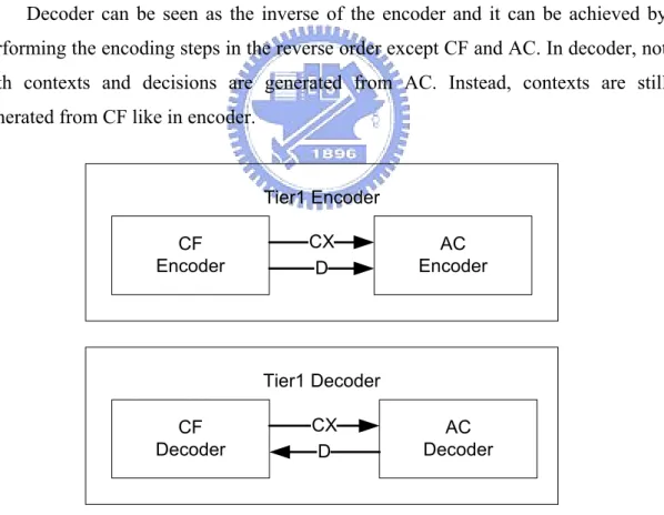
(13) CHAPTER 1. INTRODUCTION. reach 100 MHz. It can encode 2304 × 1728 image within 0.323 seconds, and decode it within 0.512 second.. 1.1.. JPEG2000 Overview. The block diagram of JPEG2000 encoder is depicted in Figure 1-1. Discrete Wavelet Transform (DWT) and EBCOT are the two main modules of JPEG2000. EBCOT coding algorithm is proposed by David Taubman [1]. It is a two-tiered coder, where Tier-1 is a context-based adaptive arithmetic coder, and Tier-2 is the rate-distortion optimization and bitstream layer formation.. JPEG 2000 EBCOT DWT. Tier-1. Quantization CF. AE. Tier-2. Figure 1-1 Block diagram of JPEG2000 encoder. In encoder, the discrete wavelet transform (DWT) is applied for the input image data. The generated coefficients may be performed by quantization process are then coded by context formation module (CF) and adaptive binary arithmetic coder (AC). Finally, the output code-stream can be executed by post-compression rate-distortion optimization algorithm (Tier-2) to reach more effective compression. During encoding, an image is divided into several rectangular structures called tiles. Either lossless 5/3 filters of DWT or lossy 9/7 filters can be applied to a tile to decompose it into several subbands. If lossy compression is chosen, the wavelet coefficients are scalar quantized. After the DWT and quantization processes, each wavelet subband is then divided into code-blocks. Each code-block is coded by context formation module. CF generates context labels and decisions to arithmetic coder. After all code-blocks are encoded independently, Tier-2 collects all bitstream with their rate-distortion information, and 2.

(14) CHAPTER 1. INTRODUCTION. then picks important bits to form the final bitstream according to rate-distortion optimization criteria. Image. Tile. tile. tile. tile. tile. Subband subband. subband. DWT. subband. Context, decision. Code-block. CF. Quantization. Codeblock. Codeblock. Codeblock. Codeblock. Compressed data. AC. Bit stream. Tier-2. Figure 1-2 Entire encoding process of JPEG2000. Decoder can be seen as the inverse of the encoder and it can be achieved by performing the encoding steps in the reverse order except CF and AC. In decoder, not both contexts and decisions are generated from AC. Instead, contexts are still generated from CF like in encoder.. Tier1 Encoder CF Encoder. CX D. AC Encoder. Tier1 Decoder CF Decoder. CX D. AC Decoder. Figure 1-3 Direction of Context (CX) and Decision (D) in encoder and decoder. 1.2.. JPEG2000 Performance. The section presents the outperformance of JPEG2000 in terms of the high 3.

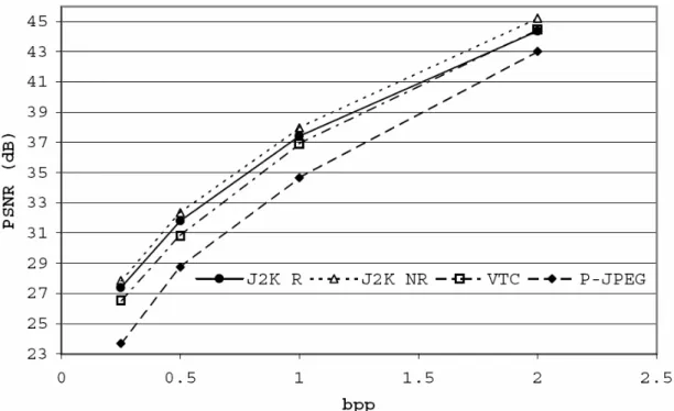
(15) CHAPTER 1. INTRODUCTION. compression ratio and various functionalities. The comparison results in this section are resulted from previous works [10]. The compared standards include reversible JPEG2000 (JPEG2000R), non-reversible JPEG2000 (JPEG2000NR), near-lossless JPEG (JPEG-LS), lossless JPEG (L-JPEG), progressive JPEG (P-JPEG), MPEG-4 VTC (VTC), and Portable Network Graphics (PNG). Lossless compression JPEG2000R. JPEG-LS. L-JPEG. PNG. bike. 1.77. 1.84. 1.61. 1.66. café. 1.49. 1.57. 1.36. 1.44. cmpnd1. 3.77. 6.44. 3.23. 6.02. chart. 2.60. 2.82. 2.00. 2.41. aerial2. 1.47. 1.51. 1.43. 1.48. target. 3.76. 3.66. 2.59. 8.70. us. 2.63. 3.04. 2.41. 2.94. average. 2.50. 2.98. 2.09. 3.52. Table 1-1 Lossless compression ratios. It can be seen that in almost all cases the best performance is obtained by JPEG-LS (except the “target” image). JPEG2000 provides, in most cases, competitive compression ratios with the added benefit of scalability. This shows that as far as lossless compression is concerned, JPEG2000 seems to perform reasonably well in terms of its ability to efficiently deal with various types of images. Progressive compression Figure 1-4 depicts the average rate-distortion behavior obtained by applying progressive compression schemes. The compared standards include JPEG2000R, JPEG2000NR, VTC, and P-JPEG. As shown in Figure 1-4, progressive lossy JPEG2000 outperforms all other schemes The progressive lossless JPEG2000 does not perform as well, mainly due to the use of reversible wavelet filters.. 4.

(16) CHAPTER 1. INTRODUCTION. Figure 1-4 PSNR corresponding to average RMSE, of all test images, for each algorithm when performing lossy decoding at 0.25, 0.5, 1 and 2 bpp of the same progressive bitstream.. Error resilience bpp 0.25 0.5 1.0 2.0. ber: 0. ber: 1e-6. ber: 1e-5. ber: 1e-4. JPEG2000. 23.06. 23.00. 21.62. 16.59. JPEG. 21.94. 21.79. 20.77. 16.43. JPEG2000. 26.71. 26.42. 23.96. 17.09. JPEG. 25.40. 25.12. 22.95. 15.73. JPEG2000. 31.90. 25.12. 22.95. 15.73. JPEG. 30.34. 29.24. 23.65. 14.80. JPEG2000. 39.91. 36.38. 27.23. 17.33. JPEG. 37.22. 30.68. 20.78. 12.09. Table 1-2 PSNR, in dB, corresponding to average RMSE, of 200 runs, of the decoded “café” image when transmitted over a noisy channel with various bit error rates (ber) and compression bitrates, for JPEG baseline and JPEG2000.. Table 1-2 compares the error resilience of JPEG2000, with the non-reversible filter, and JPEG baseline. Under the different transmission error results, the reconstructed image quality of JPEG2000 is higher than JPEG.. 5.

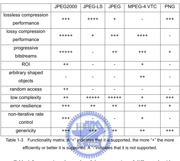
(17) CHAPTER 1. INTRODUCTION. Functionality JPEG2000. JPEG-LS. JPEG. MPEG-4 VTC. PNG. +++. ++++. +. -. +++. +++++. +. +++. ++++. -. +++++. -. ++. +++. +. ++. -. -. +. -. -. -. -. ++. -. random access. ++. -. -. -. -. low complexity. ++. +++++. +++++. +. +++. error resilience. +++. ++. ++. +++. +. +++. -. -. +. -. +++. +++. ++. ++. +++. lossless compression performance lossy compression performance progressive bitstreams ROI arbitrary shaped objects. non-iterative rate control genericity. Table 1-3 Functionality matrix. A “+” indicates that it is supported, the more “+” the more efficiently or better it is supported. A “-“indicates that it is not supported.. Table 1-3 summarizes the results of the computation of different algorithms. The table shows that JPEG2000 offers the richest set of features within an integrated algorithmic approach.. 1.3.. Thesis Organization. In this thesis, we focus on the analysis of the EBCOT Tier-1 CF algorithm, and propose an efficient block-coding engine for this critical module. The thesis is composed of six chapters. It is organized as follows. The next chapter reviews and analyses the CF algorithm of EBCOT. Chapter 3 proposes two speed-up methods, Sample-Skipping and Pass-Parallel. The architecture based on these speed-up ideas is discussed in chapter 4. Experimental results are given in chapter 5. And chapter 6 makes a brief conclusion about this thesis. 6.

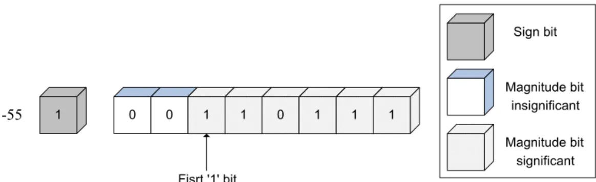
(18) CHAPTER 2. OVERVIEW OF EBCOT TIER-1 CF AND ANALYSIS. CHAPTER 2. OVERVIEW OF EBCOT TIER-1 CF AND ANALYSIS 2.1.. Context Formation module of EBCOT. Tier-1 After the DWT and quantization, each sub-band is partitioned into code-block (a rectangular grouping of coefficients typically 64×64 or 32×32 in dimension). All quantized wavelet coefficients of each code-block are expressed in sign-magnitude representation (in 1’s complement) and divided into one sign bit-plane and several magnitude bit-planes.. -31. 1. 0. 0. 0. 1. 1. 1. 1. 1. 108. 0. 0. 1. 1. 0. 1. 1. 0. 0. -55. 1. 0. 0. 1. 1. 0. 1. 1. 1. Sign bit. Magnitude bit. Figure 2-1 There are three sample with 9 bits, the first one is sign bits and others are magnitude bits. And the representation of negative is 1’s complement.. 7.

(19) CHAPTER 2. OVERVIEW OF EBCOT TIER-1 CF AND ANALYSIS. A code-block is composed of many bit-planes. A bit-plane is composed of many stripes. A stripe is composed of many columns. And a column is composed of four samples (in other words, every four rows form a stripe).. Bit-planes in a code-block. Stripes in a bit-plane. Columns in a stripe. Samples in a column. Figure 2-2 Scanning hierarchy of a code-block is bit-plane, stripe, column, sample. Each coding pass of a code-block is scanned in a particular order. The scan order of each code-block is bit-plane by bit-plane, from MSB (the most significant bit-plane with at least a non-zero element) to LSB (the least significant bit-plane), rather than sample by sample. In every bit-plane, the scanning order is stripe by stripe from top to bottom. And in every stripe, the scanning order is column by column from left to right, sample by sample from top to bottom in every column. Code-block Width. Stripe 1. Stripe 2. Stripe 3 Figure 2-3 Scan order of a bit-plane in every pass. EBCOT block coder is a context-base adaptive arithmetic coder. Each sample in each bit-plane is coded by its context and sends to the arithmetic coder along with a decision. The context of each sample is decided by five coding states, four coding primitives, and three coding passes.. 8.

(20) CHAPTER 2. OVERVIEW OF EBCOT TIER-1 CF AND ANALYSIS. 2.1.1.. Five coding states. There are five states for block coding in context formation module. They are magnitude state, sign state, significance state, refinement state, and coded state. Magnitude state The magnitude bit of every sample in the current coding bit-plane is recorded in the magnitude states. The magnitude state is different in every bit-plane for a sample. It comes from the coefficients generated from DWT in encoding. In decoder, the magnitude state is reconstructed depending on the decision generated from arithmetic decoder. Sign state The sign bit of every sample is recorded in the sign states. A zero bit indicates a positive numbers and a one bit indicates a negative numbers. The sign state of every sample is the same across all bit-planes. It also comes from the coefficients generated from DWT in encoder and also reconstructed depending on the decision generated from arithmetic decoder, just like magnitude state. Significance state A sample is called significant after the first ‘1’ bit is met while coding from MSB to LSB, and is called insignificant before the first ‘1’ bit appears, as illustrated in Figure 2-4. The significance state records if a sample is significant in the current bit-plane. It is set to one when the magnitude bit of the sample is the first ‘1’. The significance state may be changed by Pass 1 and Pass 3 coding.. Sign bit. -55. 1. 0. 0. 1. 1. 0. 1. 1. 1. Magnitude bit insignificant Magnitude bit significant. Fisrt '1' bit. Figure 2-4 A sample is called significant after the first ‘1’ bit is met.. 9.

(21) CHAPTER 2. OVERVIEW OF EBCOT TIER-1 CF AND ANALYSIS. Refinement state The refinement state indicates whether or not a sample has already been coded in magnitude refinement pass in previous bit-plane. In the beginning of coding in each code-block, refinement bits are all set to zero. And refinement bit is set to one after a sample is coded by magnitude refinement coding at first time. The refinement states may be changed only in Pass 2 coding. Coded state The coded state indicates whether or not a sample has already been coded in a previous coding pass of the same bit-plane. When a sample is coded in significance propagation pass or magnitude refinement pass, the coded state bit is set to one. After the cleanup pass, the coded state bits are all reset to zero. Note that, all the significance state bits and sign state bits are hold across all bit-planes, but the coded state bits are reset at the end of each bit-plane (in the end of Pass 3 coding). The magnitude state bits and sign state bits are coefficients from DWT in encoding, but in decoding they are reconstructed by the decisions generated from arithmetic decoder.. 2.1.2.. Four coding primitives. The context label of each sample is generated according to the status of its neighbors using four coding primitives: zero coding (ZC), sign coding (SC), magnitude refinement coding (MRC), and run-length coding (RLC). The eight neighbor samples of current sample X are separate into three groups : vertical (V0、 V1) , horizontal (H0、H1), and diagonal (D0、D1、D2、D3), as shown in Figure 2-5. The four coding operation for generating contexts are introduced below.. D0. V0. D1. H0. X. H1. D2. V1. D3. Figure 2-5 Neighbors states used to form the context. 10.

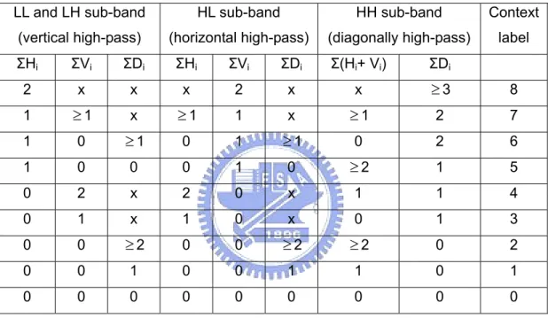
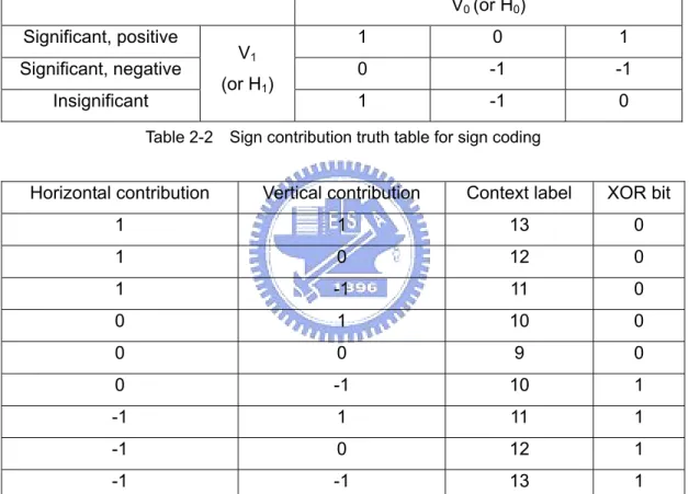
(22) CHAPTER 2. OVERVIEW OF EBCOT TIER-1 CF AND ANALYSIS. Zero Coding (ZC) The sample that is insignificant and prepares to become significant will be coded by zero coding. It is used in significant propagation pass and clean up pass. Eight neighbor samples are classified into 9 groups, corresponding to 9 contexts, as shown in Table 2-1. ΣH represents the sum of significant horizontal neighbors, ΣV represents the sum of significant vertical neighbors, and ΣD represents the sum of diagonal neighbor samples. The decision of ZC is the magnitude bit of the current sample in the bit-plane. LL and LH sub-band. HL sub-band. HH sub-band. Context. (vertical high-pass). (horizontal high-pass). (diagonally high-pass). label. ΣHi. ΣVi. ΣDi. ΣHi. ΣVi. ΣDi. Σ(Hi+ Vi). ΣDi. 2. x. x. x. 2. x. x. ≥3. 8. 1. ≥1. x. ≥1. 1. x. ≥1. 2. 7. 1. 0. ≥1. 0. 1. ≥1. 0. 2. 6. 1. 0. 0. 0. 1. 0. ≥2. 1. 5. 0. 2. x. 2. 0. x. 1. 1. 4. 0. 1. x. 1. 0. x. 0. 1. 3. 0. 0. ≥2. 0. 0. ≥2. ≥2. 0. 2. 0. 0. 1. 0. 0. 1. 1. 0. 1. 0. 0. 0. 0. 0. 0. 0. 0. 0. Table 2-1 Context table for zero coding. Sign Coding (SC) In sign coding, only vertical and horizontal neighbor samples will be used. Computation of the context label can be viewed as a two-step process. For the first step, the significance state and sign state of the vertical and horizontal neighbors are used to form the vertical and horizontal contribution, as shown in Table 2-2. For the second step, a context label and an XOR bit are formed from vertical and horizontal contributions, as shown in Table 2-3. It reduces the nine permutations of the vertical and horizontal contributions into five context labels. The decision bit that will be sent to arithmetic coder in encoding is then 11.

(23) CHAPTER 2. OVERVIEW OF EBCOT TIER-1 CF AND ANALYSIS. produced by exclusive-or the XOR bit and the sign bit. D = sign bit ⊗ XOR bit In decoding, the sign bit could be reconstructed by exclusive-or XOR bit and the decision bit generated from arithmetic decoder. Sign bit = D ⊗ XOR bit. Sign contribution. Significant,. Significant,. positive. negative. Insignificant. V0 (or H0) Significant, positive. V1. Significant, negative. (or H1). Insignificant. 1. 0. 1. 0. -1. -1. 1. -1. 0. Table 2-2 Sign contribution truth table for sign coding. Horizontal contribution. Vertical contribution. Context label. XOR bit. 1. 1. 13. 0. 1. 0. 12. 0. 1. -1. 11. 0. 0. 1. 10. 0. 0. 0. 9. 0. 0. -1. 10. 1. -1. 1. 11. 1. -1. 0. 12. 1. -1. -1. 13. 1. Table 2-3 Context table for sign coding. 12.

(24) CHAPTER 2. OVERVIEW OF EBCOT TIER-1 CF AND ANALYSIS. Magnitude Refinement Coding (MRC) The sample that has been significant in previous bit-planes will be coded by magnitude refinement coding. And it is used in magnitude refinement pass only. The context label is dependent on whether or not this sample has ever been coded in MRC and the summation of the significance state of neighbors. Table 2-4 shows the three contexts for magnitude refinement coding. The decision bit is the magnitude bit of the current sample in the bit-plane. ΣHi + ΣVi + ΣDi. First refinement for this coefficient. Context label. X. False. 16. ≥1. True. 15. 0. true. 14. Table 2-4 Context table for magnitude refinement coding. Run-Length Coding (RLC) In run-length coding, four contiguous samples in a column are coded used one context, rather than one context for each sample in other coding. RLC is used when the four contiguous samples in a column are all insignificant and their neighbors are all insignificant too. If there are fewer than four rows remaining in a code-block, then no run-length coding is used. In RLC, if none of bits of the four samples become significant, context 17 with data 0 is used. In other word, if all magnitude bits of the four contiguous samples in a column are zero, context label 17 with decision bit 0 is used sending to arithmetic coder. On the other hand, if any bit of the four samples does become significant (at least one magnitude bit of the four samples is one), context 17 with decision data 1 is used. And the first significant sample is sent using uniform coding, followed by the sign coding of the first significant sample. The rest samples of this column are coded using zero coding (same samples also need sign coding). The reason will be described later in cleanup pass.. 13.

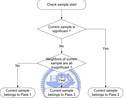
(25) CHAPTER 2. OVERVIEW OF EBCOT TIER-1 CF AND ANALYSIS. 2.1.3.. Three coding passes. There are three coding passes in each bit-plane, and they are significance propagation pass (Pass 1), magnitude refinement pass (Pass 2), and cleanup pass (Pass 3). The coding order of three coding passes is that Pass 1 is the first, Pass 2 is the next, and Pass 3 is the last coding pass in the every bit-plane except in MSB. In MSB, only Pass 3 is used (this will be explained later in this section). Figure 2-6 shows the coding order of three coding passes in a code-block. Start. Start in MSB. Pass 2 coding Pass 3 coding Pass 1 coding. Current bit-plane = Current bit-plane - 1 Current bit-plane = LSB ?. No. Yes End Figure 2-6 the coding order of three coding passes. 14.

(26) CHAPTER 2. OVERVIEW OF EBCOT TIER-1 CF AND ANALYSIS. Each sample in a bit-plane is coded in only one of the three coding passes and skipped in the other two passes. The method to determine which coding pass the current sample belongs to is illustrated in Figure 2-7. Check sample start. Current sample is significant ?. No. No. Yes. Neighbors of current sample are all insignificant ?. Yes Current sample belongs to Pass 1. Current sample belongs to Pass 3. Current sample belongs to Pass 2. Figure 2-7 Flow chart of sample checking to determine which pass a sample belongs to. Significance propagation pass Significance propagation pass (Pass 1) only includes the samples that are insignificant but have at least one immediate neighbor (V0、V1、H0、H1、D0、 D1、D2、D3) that is significant. Clearly, these samples are most likely to become significant. A sample belongs to Pass 1 is coded using zero coding. If the sample does become significant (the magnitude bit of the sample is the first ‘1’ from MSB to LSB), it also uses sign coding followed zero coding, and sets the significance bit immediately.. 15.

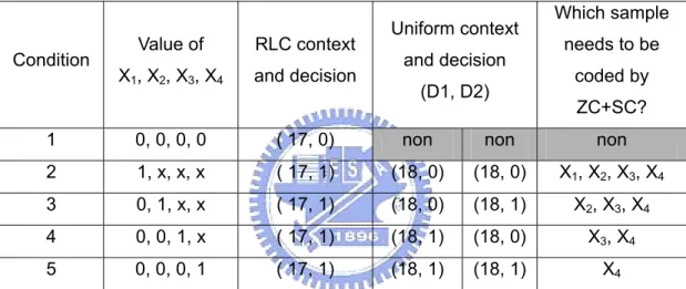
(27) CHAPTER 2. OVERVIEW OF EBCOT TIER-1 CF AND ANALYSIS. Hence, in decoding, the ZC decision received from arithmetic decoder is the magnitude bit of the sample in current bit-plane. If the ZC decision bit received from arithmetic decoder is ‘1’ that means the sample does become significant in this bit-plane. And it also needs to be coded using SC. By exclusive-or SC decision generated from arithmetic decoder and XOR bit, it could get the sign bit of the sample.. Magnitude refinement pass Magnitude refinement pass (Pass 2) includes samples that are already significant in previous bit-plane and don’t belong to significance propagation pass in the same bit-plane. The sample belongs to Pass 2 will be coded by magnitude refinement coding only. In decoding, the decision generated from arithmetic decoder is the magnitude bit of the current sample in this bit-plane.. Cleanup pass Cleanup pass (Pass 3) includes samples that don’t belong to Pass 1 and Pass 2. There are three cases in Pass 3: 1) If there is any sample in this column that does not belong to Pass 3 or not meet the RLC rule. In this case, only the ZC (or ZC and SC) is used in the samples that have not been coded in previous coding passes. 2) Suppose magnitude bits of the four contiguous samples are X1, X2, X3, and X4. If all the four contiguous samples in Pass 3 are need-to-be-coded samples and meet RLC rule, and X1, X2, X3, and X4 are all zero, then only RLC is used. 3) If all the four contiguous samples in Pass 3 are need-to-be-coded samples and meet RLC rule, but not all of X1, X2, X3, and X4 is zero. In this case, RLC, Uniform coding, and SC (or SC and ZC) are all used. Table 2-5 shows the second and the third cases in Pass 3. Condition 1 is exactly the second case. Table 2-5 condition 2~5 belong to the third case, and 16.

(28) CHAPTER 2. OVERVIEW OF EBCOT TIER-1 CF AND ANALYSIS. the uniform coding is also used in these condition. In uniform coding, it sends two context-decision pairs to arithmetic coder. Suppose the two decisions are D1 and D2. The values of D1 and C2 point out which is the first magnitude bit with the valur‘1’ from X1 to X4. If X1 is ‘1’, just like in Table 2-5 condition 2, then (D1, D2) is set to (0, 0). And the four samples with the four magnitude bits, from X1 to X4, need to be coded by ZC (except X1, it only needs to be coded by SC). On the other hand, if both X1 and X2 are ‘0’ and X3 is the first ‘1’, just like in Table 2-5 condition 4, then (D1, D2) is set to (1, 1). And the two samples with magnitude bit, X3 and X4, need to be coded by ZC (X3 only needs to be coded by SC).. Condition. Value of. RLC context. X1, X2, X3, X4. and decision. Uniform context and decision (D1, D2). Which sample needs to be coded by ZC+SC?. 1. 0, 0, 0, 0. ( 17, 0). non. non. non. 2. 1, x, x, x. ( 17, 1). (18, 0). (18, 0). X1, X2, X3, X4. 3. 0, 1, x, x. ( 17, 1). (18, 0). (18, 1). X2, X3, X4. 4. 0, 0, 1, x. ( 17, 1). (18, 1). (18, 0). X3, X4. 5. 0, 0, 0, 1. ( 17, 1). (18, 1). (18, 1). X4. Table 2-5 Contexts and decisions of the second and the third cases in Pass 3 (x: don’t care). In Pass 3 decoding, if all the four contiguous samples in this column belong to Pass 3 and meet the RLC rule, the unique RLC context is given to the arithmetic decoder. If the RLC decision returned from arithmetic decoder is ‘0’, it means the four magnitude bits are all zeros and remain insignificant. Otherwise, if the RLC decision is ‘1’, it means there is at least one of the four magnitude bits with value ‘1’. And then two uniform decisions (D1 and D2) received from arithmetic decoder denote which magnitude bit from top of the column down is the first ‘1’ magnitude bit. Note that in Pass 3 decoding, if the uniform decisions (D1, D2) received from arithmetic decoder are (0, 0), it could conjecture that magnitude bit X1 is ‘1’. Therefore, the zero coding of first ‘1’ sample can be omitted in encoding.. 17.

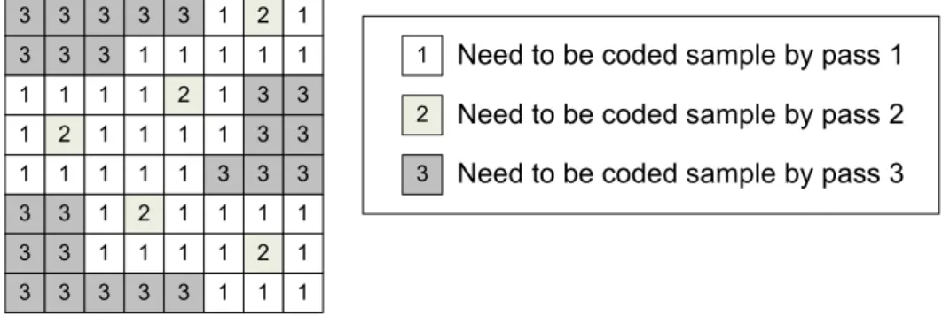
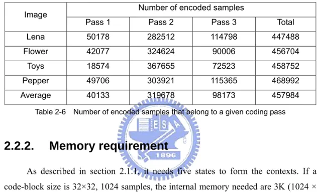
(29) CHAPTER 2. OVERVIEW OF EBCOT TIER-1 CF AND ANALYSIS. The samples in the first nonzero bit-plane are all insignificant. From the descriptions above, neighbors of all samples are insignificant, so they don’t belong to significance propagation pass. And by reason of all samples are insignificant, the magnitude refinement pass is not used in this bit-plane, too. Only cleanup pass is used in the first nonzero bit-plane.. 2.2.. Analysis of Context Formation. 2.2.1.. Execution time. As discussed in section 2.1.3, each sample in a bit-plane is checked three times, one for each pass, although each sample will be coded in only one of the three coding passes, and skipped in the other two passes. Since not all samples belong to the same pass in general case, the checking time results in a “bubble cycle”. That is, in sample-based serial checking architecture, checking four samples in a column costs four clock cycles no matter how many NBC (need-to-be-coded) samples in it. It wastes many clock cycles on processing sample location. In Figure 2-8, if each sample location requires a single clock cycle per coding pass for checking whether or not the sample is NBC sample, it wasted 29 (64-35) clock cycles in Pass 1 and 59 (64-5) clock cycles in Pass 2 and 40 (64-24) clock cycles in Pass 3. 3. 3. 3. 3. 3. 1. 2. 1. 3. 3. 3. 1. 1. 1. 1. 1. 1. 1. 1. 1. 2. 1. 3. 3. 1. 2. 1. 1. 1. 1. 3. 3. 1. 1. 1. 1. 1. 3. 3. 3. 3. 3. 1. 2. 1. 1. 1. 1. 3. 3. 1. 1. 1. 1. 2. 1. 3. 3. 3. 3. 3. 1. 1. 1. 1. Need to be coded sample by pass 1. 2. Need to be coded sample by pass 2. 3. Need to be coded sample by pass 3. Figure 2-8 There are 35 NBC samples of Pass 1 coding and 5 NBC samples of Pass 2 and 24 NBC samples of Pass 3 in a bit-plane of a 8x8 code-block. Table 2-6 shows the analysis results obtained from four 256×256, gray level test images: “Lena”, “Flower”, “Toys”, and “Pepper”. For Lena image, there are 18.

(30) CHAPTER 2. OVERVIEW OF EBCOT TIER-1 CF AND ANALYSIS. 50178 of 447488 samples encoded belong to Pass 1. It means that there are 397310 (447488-50178) clock cycles wasted for checking which sample is NBC in Pass 1, and 164976 (447488-282512) clock cycles wasted for checking in Pass 2, and 332690 (447488-114798) clock cycles for checking in Pass 3. In other words, it wastes at least 894976 (397310 + 164976 + 332690) clock cycles in coding “Lena” image. Obviously, there are a large number of clock cycles may be wasted if we use straightforward method. Number of encoded samples. Image. Pass 1. Pass 2. Pass 3. Total. Lena. 50178. 282512. 114798. 447488. Flower. 42077. 324624. 90006. 456704. Toys. 18574. 367655. 72523. 458752. Pepper. 49706. 303921. 115365. 468992. Average. 40133. 319678. 98173. 457984. Table 2-6 Number of encoded samples that belong to a given coding pass. 2.2.2.. Memory requirement. As described in section 2.1.1, it needs five states to form the contexts. If a code-block size is 32×32, 1024 samples, the internal memory needed are 3K (1024 × 3) bits (Only significance state, refinement state, and coded state need to be saved). And as described in section 2.2.1, the context information is still required in each pass even if no samples are coded in this pass. Suppose there are eight bit-planes in a code-block needed to be coded, every data in the coefficients memory will be accessed 24 (8 bit-plane × 3 coding passes) times. And the memory will total be accessed 24576 (24 × 1024 samples) times. This situation also increases the number of unnecessary memory access.. 19.

(31) CHAPTER 3. PROPOSED SPEEDUP METHOD. CHAPTER 3. PROPOSED SPEEDUP METHOD In this chapter, we will introduce two proposed speedup methods. The first one is Sample-Skipping. The Sample-Skipping method can check four contiguous samples in a column simultaneously, and avoid wasting time on non-NBC samples. The second one is Pass-Parallel. The Pass-Parallel architecture merges three coding passes of bit-plane into a single coding pass to improve the system performance.. 3.1.. Sample-Skipping. The key idea of the Sample-Skipping method is to skip no-operation samples in a single column, and directly code NBC samples. By column-based, samples in a column can be parallel checked to see whether or not they are NBC samples. It can be applied to all three coding passes. If there are n NBC samples in a column (0<n ≤ 4) , only n clock cycles will spent on coding this column, and 4-n clock cycles will be saved. If none of NBC samples is in this column, it only spends one clock cycle on checking. Since most columns have less than four NBC samples, the method can improve cycle time greatly. It is more coefficient than the straightforward method. Figure 3-1 shows the number of clock cycles spent on coding a column while Sample-Skipping is used. And Figure 3-2 shows the flow chart of Sample-Skipping.. 20.

(32) CHAPTER 3. PROPOSED SPEEDUP METHOD. NBC. 1. 1. 1. 2. 1. 2. non - NBC. 2. 3. 1. 2. 2. 3. 2. 3. 3. 4. Clock cycles required while coding the column. Figure 3-1 The number of clock cycles required while coding a column. Notice the first column, it only spend one cycle to coding a column with no NBC samples. The spent clock cycles in all kinds of columns are less than four clock cycles.. Start. There is any NBC sample in this column ?. Yes No. Code NBC sample No Has every NBC sample been coded ?. Next clock cycle. Yes End Coding. Figure 3-2 Flow chart of Sample-Skipping. 21.

(33) CHAPTER 3. PROPOSED SPEEDUP METHOD. In Sample-Skipping, data are supplied to one column at a time. We use a 6 × 3 context window instead of a 3x3 context window (just like Figure 2-5). The 6 × 3 window is illustrated in Figure 3-3, and X1, X2, X3, and X4 are the four current samples. A0, B0, C0, A1, C1, A2, X2, C2 mean the eight immediate neighbors of X1. And A1, X1, C1, A2, C2, A3, X3, C3 mean the eight immediate neighbors of X2. So are X3 and X4. A. B. C. A0. B0. C0. A1. X1. C1. A2. X2. C2. A3. X3. C3. A4. X4. C4. A5. B5. C5. Stripe n-1. Stripe n. Stripe n+1. Figure 3-3 A 6×3 context window for coding a column of samples X1, X2, X3, X4.. 3.1.1.. NBC in Sample-Skipping. In Sample-Skipping method, how to find out the NBC samples before coding a column is important. Because the values of magnitude bits can be known before encoding, and which sample will become significant in this bit-plane can be predicted. For this reason, in encoding, it could determine which sample is the NBC sample per coding pass before coding. But in decoding, it is difficult to predict NBC samples of Pass 1 and Pass 3 before coding. The condition is illustrated in Figure 3-4. Before coding, it could predict that X1 and X3 are NBC samples for Pass 1 decoding, and X2 is non-NBC for the moment. But during decoding X1, if the ZC decision generated from arithmetic decoder is ‘1’, then sample X1 will become significant and X2 will be a NBC sample. Hence, the numbers of NBC samples will change following Pass1 decoding processing. It could not predict all NBC samples before coding.. 22.

(34) CHAPTER 3. PROPOSED SPEEDUP METHOD. A. B. C Stripe n-1. X1. significant insignificant. X2. Stripe n. X3 X4. Stripe n+1 Figure 3-4 Significance state of samples in a context window before coding X1, X2, X3, X4. The condition in Pass 3 decoding is separated into two parts, RLC and non-RLC. In non-RLC, it is the same as the condition in Pass 1. In RLC, as described in section 2.1.3, it must rely on decision generated from arithmetic decoder to determine whether or not all magnitude bits are zero. And it also needs the uniform decisions to determine which sample becomes significant in uniform coding. So, in Pass 3 decoding, it is the same as Pass 1 decoding, the numbers of NBC samples will change following decoding processing.. 3.2.. Pass-Parallel. The Pass-Parallel method is to process three coding passes of the same bit-plane in parallel. There are some issues occurring due to the architecture. First, since the three coding passes work concurrently, the samples belong to Pass 3 may become significant earlier than Pass 1 and Pass 2 and this situation will mistake the following coding for samples which belong to Pass 1 and Pass 2. Second, if the sample that currently coded belongs to Pass 2 or Pass 3, the significance of samples that have not been visited in the context window shall be predicted.. 23.

(35) CHAPTER 3. PROPOSED SPEEDUP METHOD. 3.2.1.. Pass-Parallel in Encoding. To solve these issues in encoding, the coding operations for Pass 3 are delayed by two stripe columns to avoid the effect between Pass 3 and the other two passes. Subsequently, to eliminate the dependence of coding operation on the next stripe the “vertical causal” mode is also adopted. In vertical causal mode, the samples in the next stripe are considered to be insignificant. Compared with context window in Figure 3-1, the significance states of A5, B5, and C5 are considered to zero when coding X4. Figure 3-5 shows the position of context windows per coding pass in Pass-Parallel encoding architecture. Note that the context window of each coding pass is 5×3 for vertical causal mode and the context window of Pass 3 lags that of Pass 1 and Pass 2 by two columns.. Stripe. Pass 3 context window. Pass 1 context window. Pass 1 Pass 2 Pass 3. Pass 2 context window. Figure 3-5 Context windows of three coding passes in the Pass-Parallel encoding architecture. To salve the second issue, we take two states, significance state 0 (σ0) and significance state 1 (σ1), instead of significance state, refinement state and coded state. If a sample becomes significant after Pass 1 coding, the σ0 is set to ‘1’. If a sample becomes significant after Pass 3 coding, the σ1 is set to ‘1’. Besides, both σ0 and σ1 are set to ‘1’ immediately after the Pass 2 is used in this current sample. From the definition, if a sample has been coded in Pass 2, then σ0 and σ1 are both set to ‘1’. In other words, if one of σ0 and σ1 is ‘0’, it means that the sample has not been coded by Pass 2. Hence, the refinement state can be replaced by 24.

(36) CHAPTER 3. PROPOSED SPEEDUP METHOD. γ = σ0 ⊕ σ1. where ‘ ⊕ ’ is the XOR operator. (1). Obviously, the current significance state σ can be calculated during the coding process. For samples belong to Pass 1, the significance states of the visited samples are equal to σ0. Since samples that have not been visited may become significant by Pass 3 in last bit-plane, the significance states of the samples that have not been visited are expressed by σ =σ0 ∨ σ1. where ‘ ∨ ’ is the OR operator. (2). For samples belong to Pass 2, the significance states of the visited samples are equal to σ0. Since the current significant sample must be coded in Pass 2, and the neighbors of current sample must be coded in Pass 1, the neighbor sample of current sample will become significant in Pass 1 coding if its magnitude bit is ‘1’. This condition is illustrated in Figure 3-6. And the significance states of the samples that have not been visited are expressed by σ = σ0 ∨ σ1 ∨ νp. where νp is the magnitude bit. (3). significant sample the sample will be coded in Pass 2. 1. 0. 1. 0. X. 1. 1. insignificant sample with magnitude bit ｀1＇ the sample will become significant in Pass 1. 1. 0. 0. 0. insignificant sample with magnitude bit ｀0＇ the sample will maintain insignificant in Pass 1. Figure 3-6 All the neighbors will be coded by Pass 1 if the center sample belongs to Pass 2. And some neighbors with magnitude bit ‘1’ will become significant in Pass 1, the others with magnitude bit ‘0’ will maintain insignificant.. For samples belong to Pass 3, the significance states of all neighbors are determined by Equation (2). σ =σ0 ∨ σ1. where ‘ ∨ ’ is the OR operator. 25. (2).

(37) CHAPTER 3. PROPOSED SPEEDUP METHOD. 3.2.2.. Pass-Parallel in Decoding. The most difference between encoding and decoding in Pass-Parallel is Pass 2 coding. In decoding, the magnitude bit νp is generated from arithmetic decoder; therefore, it is hard to predict the significance states of the samples that have not been visited by Equation (3). To solve this problem, the coding operation for Pass 2 is delayed by two stripe columns, the same as Pass 3.. Stripe. Pass 3 context window. Pass 2 context window. Pass 1 Pass 2 Pass 3. Pass 1 context window. Figure 3-7 Context windows of three coding passes in the Pass-Parallel decoding architecture. And some equations for predicting significant states must be changed. For the samples belong to Pass 1, since the significant state σ0 of samples that have become significant in last bit-plane by Pass 3 remains to be ‘0’ after Pass 1 coding, the significance states of all neighbors are determined by Equation (2). σ =σ0 ∨ σ1. where ‘ ∨ ’ is the OR operator. (2). For samples belong to Pass 2, the significance states of the visited samples are equal to σ0 the same as encoding. Because Pass 2 delays two columns, the neighbor samples that have not been visited in Pass 2 have been visited by Pass 1. So the significance states of the samples that have not been visited are determined by Equation (2). For samples belong to Pass 3, the significance states of all neighbors are determined by Equation (2), the same as encoding.. 26.

(38) CHAPTER 3. PROPOSED SPEEDUP METHOD. 3.2.3.. Advantages of Pass-Parallel. In conclusion, the main advantages of using Pass-Parallel processing are: 1) Fast computation: No clock cycles are wasted on non-NBC samples. (Unless all of the four samples in a column are non-NBC samples. But in this case, it only spends one clock cycles on coding). 2) Less memory access: Since the three coding passed of a bit-plane are merged into a single pass, every data of memory is accessed one time for a bit-plane. And about 67% of memory accesses are saved. 3) Reduce memory requirement: We don’t need to identify whether or not each sample has been coded in a previous coding pass of the same bit-plane. The five states (magnitude, sign, significant, refinement, and coded states) are replaced by four states (magnitude, sign, significant 0, and significant 1). Therefore, the 1K (32 × 32) coded memory is saved.. 3.3.. Execution Time with Pass-Parallel. Table 3-1 shows the number of checked clock cycles in Sample-Skipping, Sample-Skipping + Pass-Parallel and the straightforward method. The four test images are the same as Table 2-6. Column “SS (P1)” represents the number of clock cycles required if the Sample-Skipping method is used in Pass 1, and so are SS (P2) and SS (P3). The last column represents the number of cycle time with straightforward method.. 27.

(39) CHAPTER 3. PROPOSED SPEEDUP METHOD. Image. Number of checked clock cycles SS(P1). SS (P2). SS(P3). SS(Total). SS + PP. Straightforward. Lena. 125260. 301893. 131053. 558206. 432185. 1211392. Flower. 121712. 335971. 114880. 572563. 443815. 1239040. Toys. 107717. 371320. 103057. 582094. 454921. 1245184. Pepper. 130682. 323847. 136892. 591421. 455503. 1275904. Average. 121343. 333258. 121470. 576071. 446606. 1242880. Table 3-1 Number of checked clock cycles in Sample-Skipping (SS) and Pass-Parallel (PP). For “Lena” image, the total number of clock cycles in Sample-Skipping method is reduced to 46% compared with straightforward method. If using both Sample-Skipping and Pass-Parallel method, the processing cycle time is reduced to 36%. Obviously, it could improve the system performance if Sample-Skipping and Pass-Parallel are applied.. 28.

(40) CHAPTER 4. ARCHITECTURE DESIGN. CHAPTER 4. ARCHITECTURE DESIGN In this chapter, we introduce the overall block diagram of Context Formation module first. The four register primitive elements (sign, magnitude, significance 0, and significance 1) are described in section 4.1. The description of context formulation module and Sample-Skipping method are discussed in section 4.2. The details of Pass-Parallel controller are in section 4.3. Section 4.4 shows the pipeline architecture.. SMW. Pass 1 coding module (P1M) Controller. Pass 2 coding module (P2M). Pass 3 coding module (P3M). CMW. RA2SD. RG. Figure 4-1 Block diagram of context formation. Figure 4-1 illustrates the block diagram of context formation (CF). It divides CF into eight blocks. The eight blocks belong to five groups as shown below:. 29.

(41) CHAPTER 4. ARCHITECTURE DESIGN. Pass Coding Module This group contains P1M (Pass 1 coding module), P2M (Pass 2 coding module), and P3M (Pass 3 coding module). The three pass coding modules produce context labels by using four register primitive elements, and produce (or receive in decoding) decisions. The Pass 1 coding module contains ZC, SC, and SS primitives. The Pass 2 coding module contains MRC and SS primitives. And the Pass 3 coding module contains ZC, SC, RLC, and SS primitives. Memory This group contains RA2SD block. RA2SD is a memory of 1024 × 2 bits. The significance state 0 and significance state 1 are saved in RA2SD. Memory read This group contains RG (Register Data Generator). The function of RG is to fill in register primitives with values loaded from two memories (four states). Memory write This group contains SMW (Significance Memory Write Module) and CMW (Coefficient Memory Write Module). The SMW block updates the value of significance state after three coding passes in each bit-plane. The CMW block only works in decoding process, it writes the value of sign bit to coefficients memory if the sample is decoded by sign coding in current bit-plane, and also writes the magnitude bits of every bit-plane to coefficients memory. Controller Controller is the core of the design. It manages the overall coding data flow, and generates write and read address for all memories and register primitive elements. It also controls the pipeline architecture.. 30.

(42) CHAPTER 4. ARCHITECTURE DESIGN. 4.1.. Column-Based Operation. In the proposed architecture, column-based operation is adopted instead of sample-based operation. The basic idea of column-based operation is to check four vertical samples of a column simultaneously. It is just like 5×3 context window in Figure 3-5 or Figure 3-7. In order to fit the Pass-Parallel architecture, it integrates context window of three coding passes into a 5×5 registers for each significance states and sign states.. Stripe. Pass 3 context window. Pass 1 context window. Pass 1 Pass 2 Pass 3 Column based registers that contains context windows of three coding passes. Pass 2 context window. Figure 4-2 Column-based registers (5 x 5). In magnitude states, it needs only four magnitude bits of four samples in current column. It doesn’t need the neighbors for magnitude state in last stripe, so the column-based registers size is 4×5.. Stripe. Pass 3 context window. Pass 1 context window. Pass 1 Pass 2 Pass 3 Column based registers that contains context windows of three coding passes. Pass 2 context window. Figure 4-3 Column-based registers (4 x 5). Take sign state registers in encoding for example. Suppose the coding order of column number is 0, 1, ..., n-2, n-1, n, n+1, n+2, and so on. By using Pass-Parallel method described in section 3.2, the coding operations for Pass 3 are delayed by two 31.

(43) CHAPTER 4. ARCHITECTURE DESIGN. columns. At time N, Column n-2 is coded in Pass 3 and column n is coded in Pass 1 and Pass 2, as shown in Figure 4-4 upper. After finishing coding column n-2 by Pass 3 and column n by Pass 1 and Pass 2 , the data registers will shift left, B to A, C to B, D to C, E to D, and new data loaded from memory is stored in the right column F. At time N+1, the column n-1 is coded in Pass 3, and column n+1 is coded in Pass 1 and Pass 2, as depicted in Figure 4-4 medium. n-3. n-2. n-1. n. n+1. n+2. A. B. C. D. E. F. n-2. n-1. n. n+1. n+2. n+3. A. B. C. D. E. Time N. Time N+1. F. n-1. n. n+1. n+2. n+3. n+4. A. B. C. D. E. F. Time N+2. Figure 4-4 Flow chart of column-based registers while time N, time N+1, and time N+2. 32.

(44) CHAPTER 4. ARCHITECTURE DESIGN. At time N+2, the data registers shifted to left again, and column n is coded in Pass 3, column n+2 is coded in Pass 1 and Pass 2. The result is depicted in Figure 4-4 lower. Note the register F in Figure 4-4. Because reading memory data needs many clock cycles, in fact, it is a ping-pong register named F1 and F2 to reduce processing cycle time. As described, there are two advantages of column-based operations: 1) samples in a column can be checked simultaneously, and then Sample-Skipping method can be applied. 2) Memory access frequency of these state variables can be reduced.. 4.2.. Pass Coding Module. The main work of pass coding module is to produce context label for arithmetic coder. In encoding, it also sends decision to arithmetic encoder, but in decoding, it receives decision from arithmetic decoder to reconstruct the coefficients memory for DWT. Pass coding module also includes Sample-Skipping architecture in it. Figure 4-5 shows the block diagram of Pass 1 coding module. The Sign Register PE, Magnitude Register PE, Significance 0 Register PE, and Significance 1 Register PE are described in section 4.1. It includes Sample-Skipping, Zero coding, and Sign coding in the Pass 1 coding module.. Sign Memory. Sign Register PE (5 x 5 bit shift register). Magnitude Memory. Magnitude Register PE (4 x 5 bit shift register). Significance 0 Memory. Significance 0 Register PE ( 5 x 5 bit shift register). Significance 1 Memory. Significance 1 Register PE ( 5 x 5 bit shift register). Pass 1 Coding SS ZC SC. Figure 4-5 Block diagram of Pass 1 coding module. 33. Context Decision.

(45) CHAPTER 4. ARCHITECTURE DESIGN. Figure 4-6 shows the block diagram of Pass 2 coding module. There are Magnitude Register PE, Significance 0 Register PE, and Significance 1 Register PE in the Pass 2 coding module (it does not include Sign Register PE), and also Sample-Skipping and Magnitude Refinement Coding in it. Figure 4-7 shows the block diagram of Pass 3 coding module. The difference between Pass 1 coding module and Pass 3 coding module is that there is a RLC block in Pass 3 coding module.. Magnitude Memory. Magnitude Register PE (4 x 5 bit shift register). Pass 2 Coding SS. Significance 0 Memory. Significance 0 Register PE ( 5 x 5 bit shift register). Significance 1 Memory. Significance 1 Register PE ( 5 x 5 bit shift register). MRC. Context Decision. Figure 4-6 Block diagram of Pass 2 coding module. Sign Memory. Sign Register PE (5 x 5 bit shift register). Magnitude Memory. Magnitude Register PE (4 x 5 bit shift register). Pass 3 Coding SS ZC Significance 0 Memory. Significance 0 Register PE ( 5 x 5 bit shift register). Significance 1 Memory. Significance 1 Register PE ( 5 x 5 bit shift register). Context Decision. SC RLC. Figure 4-7 Block diagram of Pass 3 coding module. 4.2.1.. Sample-Skipping architecture. The key idea of the Sample-Skipping method is to skip no-operation samples, and directly code NBC samples, as we described in section 3.1. In the begging of Sample-Skipping process, a NBC flag to NBC index converter is applied. The NBC flag is a four bits register, and it indicates which samples in the current coding column are NBC samples. If a bit of NBC flag is 1, it means the 34.

(46) CHAPTER 4. ARCHITECTURE DESIGN. corresponding sample is NBC; otherwise, the corresponding sample is non-NBC. The corresponding sample of the 0th bit of NBC flag is X0. And the corresponding samples of the 1st, 2nd, 3rd bits of NBC flag are X1, X2, and X3. The NBC index is an array of four integers range from 0 to 3. It is used to record the coding order of NBC samples. If X0 and X2 are NBC samples, the coding order of this column is that X0 is the first and X2 is the second, and the third and the last could be any number range from 0 to 3 because it only needs to code the first two NBC samples. So, according to NBC index, N0 (the 0th integer) is the first NBC sample in coding order. N1 (the 1st integer), N2 (the 2nd integer), and N3 (the 3rd integer) are the second, third, and the last NBC in coding order. Table 4-1 shows the NBC index converted from NBC flag. Take the 7th row for example, the value of NBC flag is 0101, and it means there are two NBC samples (X0 and X2) in this column. Obviously, the first NBC sample is X0 and the second NBC sample is X2. And the corresponding NBC index is (x, x, 2, 0). NBC flag (X3, X2, X1, X0). NBC index (N3, N2, N1, N0). 0000. x, x, x, x. 0001. x, x, x, 0. 0010. x, x, x, 1. 0011. x, x, 1, 0. 0100. x, x, x, 2. 0101. x, x, 2, 0. 0110. x, x, 2, 1. 0111. x, 2, 1, 0. 1000. x, x, x, 3. 1001. x, x, 3, 0. 1010. x, x, 3, 1. 1011. x, 3, 1, 0. 1100. x, x, 3, 2. 1101. x, 3, 2, 0. 1110. x, 3, 2, 1. 1111. 3, 2, 1, 0. Table 4-1 NBC flag converts to NBC index. 35.

(47) CHAPTER 4. ARCHITECTURE DESIGN. Figure 4-8 shows the flow chart of Sample-Skipping method. The current NBC sample is N0 if ‘I’ equals to 0. And the current NBC sample is N1, N2, or N3 if ‘I’ is 1, 2, or 3. In the begging of the flow, set ‘I’ to be zero, and check if there is any NBC sample in this column. If none, finish coding in this column. Otherwise, it means that there is at least one NBC sample, and the first NBC sample (N0) is coded immediately. After generating context label of the NBC sample, increase ‘I’ by one, and check whether or not the number of NBC samples is equal to ‘I’. It means total NBC samples have been coded already if ‘I’ is equal to the number of NBC samples. So, if number of NBC samples equals to ‘I’, finishing coding in this column; otherwise, coding the next NBC sample (N1) at next clock cycle and follows the flow until all NBC samples have been coded. Start. I=0. Number of NBC = 0 ? No Find out the current NBC sample by index I. Code the current NBC sample. No. Yes I=I+1. I = Number of NBC ?. Next clock cycle. Yes End Coding. Figure 4-8 Flow chart of Sample-Skipping architecture (include of finding out the current NBC sample by index I). 36.

(48) CHAPTER 4. ARCHITECTURE DESIGN. Only in Pass 2 decoding, the NBC samples could be checked before starting coding. The NBC samples of Pass 1 and Pass 3 decoding may be changed according to the decision from arithmetic coder. Therefore, the MRC (or the Pass 2 coding) is the simplest coding of four coding primitives. Let’s introduce the Pass 2 coding module first.. 4.2.2.. Pass 2 coding module architecture. Figure 4-9 shows the flow chart of Pass 2 coding module, it’s similar to the flow chart of Sample-Skipping.. Pass 2 Codec Start. MRC. I=0. Number of NBC = 0 ?. No Generates context label of current NBC sample. Decoding No. Encoding Receive decision from AC?. Generate decision of current NBC sample Yes I=I+1. Yes. I = Number of NBC ? Yes Pass 2 Codec End. Figure 4-9 Flow chart of the Pass 2 coding module (MRC). 37. No.

(49) CHAPTER 4. ARCHITECTURE DESIGN. While there is at least one NBC sample in this column, the Pass 2 coding module will generate context label, and then there are two directions. The green one is for encoding. It is the same as Sample-Skipping flow chart while following the green direction. The purple one is for decoding. Following the purple one, it does not provide decision to arithmetic decoder. On the contrary, it waits for the decision generated from arithmetic decoder. Until receiving the decision from arithmetic decoder, it goes on with the flow chart.. 4.2.3.. Pass 1 coding module architecture. Figure 4-11 shows the flow chart of the Pass 1 coding module, and it is also the flow chart of zero coding and sign coding. Note that the previous section of Figure 4-11 is similar to the flow chart of the Pass 2 coding module. But after generating decision in encoding or receiving decision from arithmetic decoder in decoding, it has to check whether or not the sample needs to be coded in sign coding by the value of decision (i.e. ‘1’ means that needs be coded by SC, and ‘0’ means that does not need be coded by SC). If the SC is needed, it must generate the context label of SC, and receive the decision of SC from arithmetic decoder. The rest flow path of Pass1 coding is similar to Sample-Skipping flow chart.. 4.2.4.. Pass 3 coding module architecture. The coding primitives of Pass 3 coding are SC, ZC, and RLC. Since the SC and ZC in Pass 3 coding and Pass 1 coding are the same, in this section, we focus on the flow of RLC (and the uniform coding). The path of flow chart, as depicted in Figure 4-10, also has two directions which green one for encoding and purple one for decoding. Following green paths (encoding paths), Pass 3 coding module generates run-length context label (17) and decision. If none of the magnitude bits in the column is 1, the four samples do not need to be coded by uniform coding, and Pass 3 coding in this column is finished. Otherwise, it means the four samples needs to be coded using uniform coding. After sending two uniform context labels (18) to arithmetic 38.

(50) CHAPTER 4. ARCHITECTURE DESIGN. encoder, RLC and uniform coding in this column are finished. And the rest of NBC samples will be coded by ZC and SC. Following purple paths (decoding paths), it generates run-length context label (17). If the RLC decision received from arithmetic decoder is zero, it means that none of the four magnitude bits in this column is 1, and finishes Pass 3 coding in this column. If the RLC decision received from arithmetic decoder is one, then not all four magnitude bits are zero, and this column needs to be coded using uniform coding. According to the two uniform decisions generated from arithmetic decoder, it could determine how many samples needed to be coded by ZC and SC.. Pass 3 RLC Codec Start. Generates context 17. RLC. Decoding. No. Encoding Receive decision from AC?. Generates decision. Need uniform contexts ?. Yes. Yes Generates context 18. Decoding No. Encoding No. Receive decision from AC?. Generates D1 decision Yes Generates context 18. Decoding No. Encoding Generates D2 decision. Pass 3 Codec End. ZC and SC. Receive decision from AC?. Yes. Figure 4-10 Flow chart of Pass 3 coding (RLC). 39.

(51) CHAPTER 4. ARCHITECTURE DESIGN. Pass 1 Codec Start. ZC + SC. I=0. Number of NBC = 0 ?. No Generates ZC context of current NBC sample. Decoding No. Encoding Receive decision from AC?. Generate ZC decision of current NBC sample. Need SC ?. Yes No. Yes. Yes. Generates SC context of current NBC sample No. Decoding No. Encoding Receive decision from AC?. Generate ZC decision of current NBC sample. I=I+1. Yes. I = Number of NBC ? Yes Pass 1 Codec End. Figure 4-11 Flow chart of Pass 1 coding (ZC+SC). 40.

(52) CHAPTER 4. ARCHITECTURE DESIGN. 4.3.. SMW and CMW Architecture. After a column is processed by three coding passes, the memories must be updated if there are any changes in the significance states, or coefficient states. The SMW (Significance Memory Write Module) is used for updating the value of significance states. The CMW (Coefficient Memory Write Module) is used for updating the value of magnitude and sign states, and CMW only works in decoding. Significance Memory Write Module (SMW) Figure 4-12 shows the flow chart of SMW. It is similar to the flow chart of Sample-Skipping depicted in Figure 4-8. The only difference between them is that SMW changes “Code the current NBC sample” to “Write data to memory”. The index NBCH is used to record if the sample is a need-to-be-changed-value sample, just like NBC. Start. I=0. Number of NBCH = 0 ?. No Write data to memory Yes. No. I = I +1. I = number of NBCH ?. Next clock cycle. Yes End Coding Figure 4-12 Flow chart of writing new significance states into memory. 41.

(53) CHAPTER 4. ARCHITECTURE DESIGN. The significance memory (RA2SD) is composed of significance state 0 and significance state1, and it is a 1024 × 2 bits memory. The 0th bit represents the significance state 0, and the 1st bit represents the significance state 1. The data prepared for writing into significance memory RA2SD is combined from significance 0 register and significance 1 register. Coefficient Memory Write Module (CMW) Start. I=0. Number of NBCH = 0 ? No read data from memory Next clock cycle Combine data with magnitude and sign register. Yes write data to memory. No. I = I +1. I = number of NBCH ?. Next clock cycle. Yes End Coding Figure 4-13 Flow chart of writing coefficients into memory. It is similar to the flow chart of writing significance states into memory. But the data must be loaded from memory before writing.. 42.

(54) CHAPTER 4. ARCHITECTURE DESIGN. CMW works only in decoding process. It is a little different between SMW and CMW. After three passes coding, we could get a magnitude bit of a sample in current bit-plane and maybe the sign bit if the sample is coded in SC at the bit-plane. The coefficient memory is a 1024 × 9 bits memory, 1 bit for sign bit and 8 bits for magnitude bits. In the magnitude register, it only could record one magnitude bit for a sample. So, it could not get coefficient data by combining the two register. In CMW, before writing data to memory, it needs to read data from memory. And then store the magnitude bit and sign bit into the current position of data. According to this concept, the CMW costs more clock cycles than SMW.. 4.4.. Pipeline. Recall the column-based registers, in the encoding, the register B is coded using Pass 3 coding, and register D is coded using Pass 1 and Pass 2 coding, as described in section 4.1. The sample which has been coded by three coding passes will shift to register A, and SMW will update significance memory by the data of four samples in register A. The register F is stored of data loaded from memory by RG. Figure 4-14 shows the relation of five blocks (P1M, P2M, P3M, RG, and SMW) and six registers in encoding. P1M SMW P3M. P2M. RG. n-3. n-2. n-1. n. n+1. n+2. A. B. C. D. E. F. Time N. Figure 4-14 Relation of five blocks and six registers in encoding. In decoding, Pass 2 coding module delays two columns to register B. And 43.

(55) CHAPTER 4. ARCHITECTURE DESIGN. register A is coded also by CMW. Figure 4-15 shows the relation of six blocks (P1M, P2M, P3M, RG, SMW, and CMW) and six registers. CMW P2M SMW P3M. P1M. RG. n-3. n-2. n-1. n. n+1. n+2. A. B. C. D. E. F. Time N. Figure 4-15 Relation of six blocks and six registers in decoding. From Figure 4-14 and Figure 4-15, we know that if every module finishes its work in the corresponding register, the data of registers will shift left. According to this concept, pipeline architecture is easy to implement. Figure 4-17 is the flow chart of pipeline architecture. The code-block size is 8 × 7, 7 columns and 8 rows. We define the index of every sample as follows.. 0. 1. 2. 3. 4. 5. 6. 32. 33. 34. 35. 36. 37. 38. 64. 65. 66. 67. 68. 69. 70. 96. 97. 98. 99. 100. 101. 102. 128. 129. 130. 131. 132. 133. 134. 160. 161. 162. 163. 164. 165. 166. 192. 193. 194. 195. 196. 197. 198. 224. 225. 226. 227. 228. 229. 230. Figure 4-16 Index of every sample for a 8 x 7 code-block. 44.