Simulating Time-Varying Demand Services with
Queuing Models
Hsuan-Kai Chu
∗, Wan-Ping Chen
†and Fang Yu
∗∗Department of Management Information Systems, National Chengchi University, Taipei, Taiwan 116
Email:see http://soslab.nccu.edu.tw/Contact.html
†Institute of Statistics, Academia Sinica, Taipei, Taiwan
Abstract—Resource provision for services that have time-varying demands has raised a great concern to service providers aiming at high-standard service quality. We propose a new resource provision approach using service simulation and arrival rate estimation that integrates unsupervised clustering and statis-tics techniques. We first cluster days that have similar arrival patterns together, where from each cluster we can reveal and separate days having different reasons for time-varying demands of the service. We then adopt the two layer business factor model to estimate multi-interval Poisson arrival distributions on daily bases for simulating stochastic processes. Applying simulation on queuing models with multi-interval Poisson arrival processes, we can observe stochastic changes of customer waiting time, queuing lengths and number of workers under different service strategies. We conduct a case study on an electricity service call center in real industries, showing how to build adequate resource provision and estimation against history data in past years and how the performance improved compared to their previous heuristics in real life operations.
Index Terms—Arrival rate estimation, Service simulation, Time-varying demands, Resource provision
I. INTRODUCTION
Cloud computing has affected lives everywhere. While cloud computing platforms have been widely adopted as solu-tions to provide scalable services in recent years, management of cloud-based services [1] faces a great challenge of on-demand resource provisioning and allocation in response to time-varying workloads. These demands are stochastic because of customer randomly requests. According to NIST [2], cloud computing is a model for enabling ubiquitous, convenient, on-demand network access to a shared pool of configurable com-puting resources (e.g., networks, servers, storage, applications, and services) that can be rapidly provisioned and released with minimal management effort or service provider interaction. facilitate dynamic resource reallocation according to service demands [3]. Cloud computing allows companies to start small and increase hardware resources only when there is an increase in their needs. Because of the ability to pay for use of comput-ing resources on a short-term basis, providers of cloud-based services are rewarding conservation, having machines and storage come and go on demand. Virtual machines (VMs) that can be instantaneously cloned as multiple replicas running on the same or different physical host facilitate dynamic resource reallocation. As a result, cloud computing enables ubiquitous, convenient and on-demand network access to a shared pool
of configurable computing resources (e.g., networks, servers, storage, applications and services) [2].
Still in practice, e.g., Elastic Compute Cloud (EC2) from Amazon Web Service (AWS) [4], [5], service providers are asked to provide resource reservation plans in a long-term lease. Experimentation of cloud computing in a real environ-ment is expensive, time costly and not repeatable [6]. The cost could be increasing significantly observing poor system performance and worse clients’ experiences after actually launching and running the services under the reservation plan. To have a systematic estimation of the effects of adjustment on the workloads and the cost of each hour or day with time-varying demands, simulation poses an attractive solution that provides observations of the stochastic processes of a relatively closely-estimated system of cloud services.
The estimations can be used to build adequate reservation plans without launching the service. It is essential that the service provider has suitable resource provision regarding the cost and the quality of service, having sufficient amount of resources allocated to meet service agreements. On the other hand, through the simulation, the service provider can also observe clients’ experiences with varying demands when the server runs different reservation plans or strategies. Neverthe-less, setting a simple reservation policy, e.g., a heuristic sched-ule to dispatch resources in various periods, may directly lead to under-provisioning or over-provisioning of resources [4].
To improve the precision of resource provision, we propose a systematic approach for synthesizing workloads of daily reservation policy under different service quality strategies through arrival rate estimation and service simulation. The simulation shows the stochastic processes under the esti-mated arrival distributions, providing information for service providers to build a reservation plan, e.g., the number of VMs to fulfill the demands in each period, and hence prevent under or over-provisioning situations.
In this work, we are particularly interested in time-varying demand services on daily basis. Specifically, given history data on arrivals, we first divide a day into several equal length periods and accumulate the arrivals in each period. The arrival pattern of a day is then considered as a high dimension vector with attributes as periods and values as the number of arrivals in each period. These day arrival patterns may vary due to the dates of the day, e.g., weekends, or unusual events that happened in the day, e.g., typhoons and earthquakes.
To characterize different day patterns, we adopt unsupervised clustering on each day according to their arrival pattern. Days that fall in the same cluster have similar arrival patterns in a day.
We then adopt the two layer business factor model [7] to estimate distributions of each period as the day arrival pattern of each cluster for simulating the stochastic process. The two-layer model reflects the busy level of a day and its relations among periods within a day. After having the estimated arrival distributions, we simulate the stochastic processes to observe the workload of a day under different resource reservation plans and strategies.
Finally, we conduct a case study on an electric service company in Taiwan. We collect thousands of logs of their history call data from their call center from 2012 to 2015. The arrival patterns are clustered into five groups; from these clusters we can check history data and identify features of these days, such as weekends, regular working days, and days that have unusual events happened with severe damages. We estimate the arrival patterns for each cluster and the service rate for simulating the stochastic process. We propose two strategies to allocate resources dynamically and report the number of virtual machines that are needed in different periods, as well as average waiting time and queue lengths during the simulation. Compared to the system performance of the reservation plan that is is adopted by the company in real life, we show that we can improve the service performance by adopting dynamic allocation strategies.
The rest of the paper is organized as the following: we summarize previous related work in Section 2, present the methodology of clustering, estimation, and simulation in Sec-tion 3, and conduct the case study in SecSec-tion 4, and conclude the work in Section 5.
II. LITERATUREREVIEW
We briefly review previous work in cloud simulation, re-source provision and arrival rate estimation in this section. A. Cloud Simulation
Calheiros, Ranjan, Beloglazov, De Rose and Buyya [8], [9] proposed the most famous simulation toolkit CloudSim for modeling and simulation of cloud computing environments. CloudSim supports system and behavior modeling of cloud computing system components. CloudAnalyst built based on CloudSim is proposed by Wickremasinghe, Calheiros, and Buyya [10], [11] for supporting the visual modeling and simulation of large-scale applications on cloud infrastructure. It provides more description of the application including the geography information and number of resource in each center and traffic by user location. Garg and Buyya [12] propose NetworkCloudSim that extends the CloudSim with a scalable network model. NetworkCloudSim can be used to model the cloud computing environment where the application and its customers are different without communication tasks or lim-ited network model within the data center. EMUSIM is built based on Automated Emulation Framework and CloudSim
to predict service behavior on a cloud platform. A detailed comparison can be found in [13]. Other than CloudSim related simulation tools, Kliazovich, Bouvry, and Khan pro-pose GreenCloud [14] that targets on the energy costs of the data center. Lim, Sharma, Nam, Kim, and Das propose MDCSim [15] that is specific in hardware characteristics of different model components of the data center. Our simulation platform takes advantage on arrival rate estimation, providing precisie resource provision for time-varying demand services. B. Resource Provision
Many researchers have developed various resource provi-sioning frameworks. Most of them try to solve the uncertainty and intensity vary widely of the arrivals. In this section, there are some study and practice in resource provisioning of distributed system addressed in [16], [17], [18], [19], [20], [4].
Jamshidi, Ahmad, and Pahl [16] exploit a fuzzy logic to handle unexpected spikes in the workload and provide the acceptable user experience. It also describes the uncertainty in cloud-based software, and some approaches do not explicitly deal with the situation that unexpected events are frequent. Ku-sic and Kandasamy [17] develops a framework for optimizing the resource provisioning problem using a limited lookahead approach [21]. It also mentions that the France World Cup web site [22] show up to 20% more profit per day using the framework.
Lim, Babu, and Chase [18] propose a controller for an elas-tic storage system based on the Hadoop Distributed File Sys-tem (HDFS). It focuses the resource provision of storage tier under dynamic Web 2.0 workloads. Bennani and Menasce [19] point out that some resource provisioning approaches will face the problem of scalability limitations and the arrival is untraceable. It provides an alternative solution based on the use of analytic queuing network models and demonstrates the performance of the approach.
Chaisiri, Lee, and Niyato [20] proposed an optimal virtual machine placement (OVMP) algorithm. OVMP can minimize the cost of hosting virtual machine in multiple cloud provider environment under future demand and price uncertainty. An-other algorithm motivated by OVMP, Chaisiri, Lee and Niyato update an optimal cloud resource provisioning (OCRP) algo-rithm for virtual machine management in cloud computing. The algorithm considers the provisioning stages and prices for a user using computing resource significantly.
C. Arrival Rate Estimation
Zhang, Jiang, Yoshihira, Chen, and Saxena [23] propose the best use of cloud service based on the workload (or a number of request arrives) estimation. They study the dynamics of hourly workload measuring during a 46-day period of the on-line video sharing website provided by Yahoo [24]. Avramidis and L’Ecuyer [25] describe the arrival rate uncertainty of a call center, modeling and estimating its arrival rate and service times. Roy, Dubey, and Gokhale [26] proposed a predictive model with workload forecasting in cloud system to develop an
auto-scaling resource provision using auto-regressive moving average method (ARMA). Cunha, Almeida, Almeida and San-tos [27] combine an adaptive capacity management framework for system performance. It assumes request arrivals following non-homogeneous Poisson process with rate changes. We adopted the two-layer model proposed by Oreshkin, Regnard and L’Ecuyer [7] for modeling the relationships among periods in a daily base.
III. METHODOLOGY
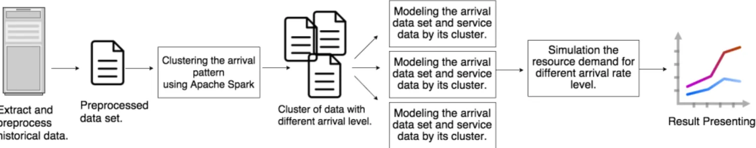
We present our methodology in this section. The process can be divided into three stages. The first stage is to extract and cluster arrival patterns for daily calls. The second stage is arrival rate modeling to estimate distributions of arrivals in periods of each day. The last stage is the stochastic simulation procedure with queuing models. Figure 1 shows the overview of our analysis architecture. We detail each stage in the following sub sections.
A. Arrival Pattern Clustering
Demands are varied day by day. The daily arrival pattern may vary due to various reasons such as regular work-day/weekends, accidents, unpredictable damages, policy ad-justments and rate changes of system operations, etc. However, there may be some patterns that are shared with days. To figure out days that have similar arrival patterns, we apply unsupervised clustering on daily arrival patterns (that could be extracted from raw log files as we will show in the case study) and apply the arrival rate estimation on days that have similar arrival patterns. We formally define arrival patterns in the next section.
As for clustering, we adopt K-Means [28] algorithm to fulfill the purpose of arrival pattern clustering. Specifically, to deal with a potential large amount of data, we incorporate our implementation with the Spark MLlib [29], a distributed machine learning library for large-scale data processing. The tool set is well-suited for iterative machine learning tasks with APIs available for Java, Scala, Python, and R [30].
B. Arrival Rate Modeling and Estimation
We adopted the estimation method proposed by Oreshkin, Regnard and L’Ecuyer [7] for modeling the arrival rates. It assumes that the customer arrival historical data is existing. We then consider the operation time of the system and divid it into p multiple periods of equal length. For example, if the system receives the request from 00:00 to 24:00 and each period has 30 minutes, we have p = 48. Let Y = (Y1, Y2, ..., Yp) be the vector of arrival counts in those p periods. It assumes that the arrivals are from a Poisson process with a random rate Λ = (Λ1, Λ2, ..., Λp) having an arbitrary multivariate distribution over [0, ∞)p. Taking its mean λ = (λ
1, λ2, ..., λp) as a scaling factor or base rate, and Λj = Bjλj where Bj is a non-negative random variable called busyness factor having B = (B1, B2, ..., Bp) with E[Bj] = 1 for each j. To summarize, it has
Λj= Bjλj and Yj∼ P oisson(Λj)
where Yj’s are independent and each Yjhas a Poisson distribu-tion with mean Λj, and the Poisson distribution with mean λj denoted as P oisson(λj). However, this model is non-standard, because the rates Λj are hidden and can be inferred only indirectly through the counts Yj, and its parameters are often hard to estimate for this reason.
We adopt the two-layer model in this work. Based on the multiplicative combination of independent period of busy-ness factor ˜Bj and the busyness factor for the day, ¯B, let Gamma(a,b) denote a gamma distribution with mean a/b and variance a/b2. They assume that ¯B, ˜B
1, ..., ˜Bpare independent with
¯
B ∼ Gamma(β, β) and B˜j ∼ Gamma(αj, αj) for each j and for some positive parameters β, α1, ..., αp. It take
Bj = ˜BjB¯j
as the busyness factor of period j. This combination permits one to better control the correlation between the Bj’s, in comparison with the previous special cases where it was either 0 or 1.
Simple formulas are available for the moments in this model: V ar(Bj) = (1 + β + αj) βαj (1) and Cov(Bj, Bk) = 1 β (2)
Those additional terms for the Two-Layer model provide more flexibility to match the variances and correlations. They choice Maximum likelihood estimators (MLEs) for estimating the parameters because MLE is generally more robust and accurate in experience. While these estimators were readily available for the previous special cases, here they are much harder to compute. More specifically, the available expression for the density of Yj, which appears in the likelihood function for each j, involves an integral with respect to the realization of the vector of unobserved daily busyness factors and do not know how to evaluate this integral in closed form. They opted to develop parameter estimation methods for this model based on Monte Carlo estimation of the loglikelihood function.
The Algorithm 1 shows the estimation of arrival rates in a two-layer busyness factor modeling. We initialize the gamma parameter estimator with the arrival pattern dataset first, and then we find the busyness factor of the day in the dataset ¯B by using the function GammaParameterEstimator to sample a gamma value with the parameter β. The parameter β is for sampling a global busyness factor. For each period of a day, we find the busyness factor of each period j as ˜Bjby sampling a gamma value with parameter αj. The parameter αj is the parameter for sampling a value from the gamma distribution in each period. The final busyness factor of each period is B[j] = ¯B* ˜B[j]. The final poisson distribution of period j is defined with Λ[j] that is returned by the algorithm.
Figure 1. Architecture of Simulation Platform
Algorithm 1 Arrival rate estimation input: Arrival[date][count] output: Λ[j], j = 1, . . . , p 1: GP E = GammaP arameterEstimator(Arrival) 2: β = GP E.getB() 3: B = gamma(β, β).sample()¯ 4: α[j] = GP E.getα() 5: f or all j: 6: B[j] = Gamma(α[j], α[j]).sample()˜ 7: B[j] = ¯B* ˜B[j] 8: Λ[j] = λ[j] ∗ B[j] 9: return Λ[j]
C. Stochastic Simulation with Queuing Models
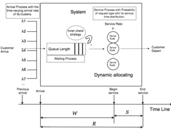
We present our stochastic simulation procedure based on the queueing models in this section. Figure 2 shows the overview of pour simulation structure with queuing models. The method shows the service quality of the system for various parameter setting, for example, arrival rate in each period, service rate, the quality of service bound including average waiting time and queue length.
The procedure of simulation including three parts: The simulation method for the system, the arrival event, and service completion event. Table I specifies the parameters used in the simulation procedure. Algorithm 2 is the main procedure for simulation. Before the while loop, initialize the parameter, server list and the boolean flag arrivalEvent and serviceEvent to F alse, which means the event in this cycle is not decide yet in every cycle begin. Phase 1 starts the procedure while the clock in simulation does not reach end time.
Phase 2 to Phase 9 is updating the clock in the simulation. If the hour in simulation does not change, sum up the parameters like the number of servers in the system for estimate quality of service. If not, the list will save the average number of server, queue length in this hour and update the parameters. Phase 10 gets the first free server id in the server list. Phase 11 gets the id having the first completion time in the server list. Phase 12 to Phase 17 identify the event type of this cycle. We have several steps here. First, we will get the index of the server which has lowest service completion time from the server list and get its service completion time NCT also (The first time
Table I
DESCRIPTION OF PARAMETERS IN THE SIMULATION PROCEDURE
Name Definition
W The cumulative experienced waiting time in the queue.
Q The queue save arrival event time.
arrivalEvent The Boolean value to decide the event is arrival event.
serviceEvent The Boolean value to decide the event is service event.
qLength The bound number of customer waiting in the queue. wBound The bound of customer waiting time.
nat The next arrival time in the simulation procedure. nct The next completion time in the simulation
proce-dure. s
An server s has two fields: s.state indicates the server status is busy or not and s.nct indicates that the next completion time of service by a server.
S The list of servers that store those servers’ status. E[W] The average waiting time.
prevClock The prevent event time in the simulation procedure. clock The current event time in the simulation procedure. ts The number of total served
te The number of total events.
of cycle will set to 0). After that, we find the earlier time of next customer’s arrival time NAT and NCT, the earlier one will be the event type in this cycle, set the arrivalEvent or serviceEvent to T rue.
Phase 18 updating the time in the simulation, setting the prevent event time to the clock, and clock time to this event time. Phase 19 will also be a check that whether the quality of service bound is met. This constraint is that the queue is no longer than qLength customers or the waiting time of a person are over than wBound minute. If it is not, the Boolean flag createStatus will be set to F alse, or set to T rue, otherwise. The flag createStatus is used to identify should add a new server to server list or not. The further description shows in section E.
Phase 20 will lead the procedure to Algorithm 3 if the arrivalEvent is T rue or Algorithm 4 if the serviceEvent is T rue. After the while loop end, return the quality of service parameter we concerned. The view of our simulation structure shows in Figure 2.
Algorithm 3 is invoked when arrivalEvent is T rue in Algorithm 2. First, we sample a next arrival time NAT by adding a random number which following the exponential distribution having lambda change based on the current clock
Figure 2. An overview of the simulation structure with queuing models.
in simulation if it does not exceed the end time (If NAT reach the end time, setting the NAT to IN F IN IT Y for break the while loop). Second, we check if there is at least one server free by inner conditional loop by using the parameter idF ree mentioned above. If idF ree equal to -1 means that there is no available server in the server list, so we put the customer into the queue and if createStatus is TRUE, add a new server to the server list. If idF ree not equal to -1 means that there is at least one server is free and ready to serve. We set the server state to busy with idF ree and sample for the time of its next service completion time, put it back to the server list. Third, we check if the queue is empty. If so, the total served customer is increased by 1.
Algorithm 4 is invoked when serviceEvent is T rue in Algorithm 2. A service completion event has two cases; the queue is being empty or not. The two situation will lead to different behaviors in the simulation. Case 1: the queue is empty. First, we check the createStatus and size of server list. If the createStatus is F alse and size is more than the initial number of server, we remove the server with idF ree meaning that the retirement of the server. Second, get the first busy server and release them by setting its state to free and its next completion time to IN F IN IT Y which means that set the server to idle and have priority to be the next free server. Or the situation 2, the queue is not empty. It means that there is some customer waiting in the queue. In this situation, first, we get out the customer from the queue and record the time that the customer arrival to system t. The waiting time of the customer is clock–t. Second, we take a sample for the next service completion time NCT using the current time + a random number from an exponential distribution having µ, and we also provide other distribution for different services. Getting the server having the lowest NCT meaning that it is the first server that able to start next service, setting the new NCT into it and put it back to the server list. At the end of the cycle, increment the number of total events and if this is neither arrivalEvent nor serviceEvent, set the NAT to IN IF IN IT Y to break the while loop.
Algorithm 2 The main simulation procedure Input: arrival rate, service rate, QoSBound. Output: avgWait, avgLength, AvgServerNum
Initialization : NT, W, L, t, clock = 0. arrivalEvent, serviceEvent = False. Initialized the Queue Q and servers S status.
1: while clock < endT do
2: currHour = (int) clock
3: if (currHour == prevHour) then
4: serverSum+ = servers, qSum+ = Q.length()
5: else
6: AvgServerN um.add(serverSum/(te −
hourStartEvent))
7: AvgLength.add(qSum/(te − hourStartEvent))
8: serverSum = 0, hourStartEvnet = te, prevHour = currHour
9: end if
10: idF ree = getN extF reeServerId() 11: idN CT = getN CT Id()
12: nct = S.get(idN CT ), e.time = min(nat, nct)
13: if e.time = nat then
14: arrivalEvent = T rue
15: else
16: serviceEvent = T rue
17: end if
18: prevClock = clock, clock = net.time
19: createStatus = (QoSReachBound)?true : f alse)
20: if (arrivalEvent) then
21: Call Algorithm 3; arrivalEvent = F alse;
22: end if
23: if (servicelEvent) then
24: Call Algorithm 4; servicelEvent = F alse;
25: end if 26: te = te + 1
27: end while
28: return AvgW ait=W/ts, AvgLength, AvgServerN um
Algorithm 3 Arrival event process.
1: λ = getLambda(net.time)
2: Create a next arrival time nat = clock + nextExponential(λ).
3: if idF ree! = −1 then
4: getServer(idF ree).setN CT (clock +
nextExponential(µ))
5: getServer(idF ree).setState(busy) 6: else
7: Q.put(clock)
8: if (createStatus = T rue) S.add(new server) 9: end if
10: if Q.isEmpty() then
11: ts = ts + 1
12: end if
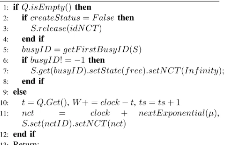
Algorithm 4 Service-completed event process.
1: if Q.isEmpty() then
2: if createStatus = F alse then
3: S.release(idN CT )
4: end if
5: busyID = getF irstBusyID(S)
6: if busyID! = −1 then
7: S.get(busyID).setState(f ree).setN CT (Inf inity);
8: end if 9: else 10: t = Q.Get(), W + = clock − t, ts = ts + 1 11: nct = clock + nextExponential(µ), S.set(nctID).setN CT (nct) 12: end if 13: Return;
D. Dynamic Resource Provision
Our simulation platform provides dynamic resource alloca-tion that are determined according to the provision resource strategy. We have two strategy parameters that can be adjusted as the trigger to initialize a new server node. The first parameter is the current length qLength of the waiting line and the second is the average waiting time wBound of a customer. The strategy of the resource provision is to set the bound value of qLength and wBound. In the simulation procedure, we set these two parameters first for estimation of the quality of service, and we then observe the average waiting time, the queue maximum length and the number of customer waiting for more than wBound, and the average server nodes used in different periods. When it happens that the bound of the length of the waiting line or the waiting time of a customer is reached, a new server is added to the system to improve the quality of service. This strategy called dynamic provision provides service providers the on-demand resource allocation. We have implemented the simulation platform described in this section. In the next section, we present a case study to illustrate our idea with real log data and to show the results and performance comparison on simulation against dynamic resource provision and static resource provision according to heuristics in practice.
IV. CASESTUDY
In this section, we conduct the case study on an electricity service call center, showing how we perform the clustering, arrival pattern modeling and estimation and hence build ad-equate resource provision and estimation, showing how the performance improved compared to the previous methods. A. Log Preprocess Stage
We have collected data directly from the system used in the call center from 01/01/2012 to 12/31/2015, with a total number 4080000+ call records in system logs. A fraction of the raw data is shown in Figure . In this stage, we first preprocess the data to extract the information for arrival rate estimation.
Figure 3. An Example Of Log Files
Each record in the raw data has the exact date and time when the call comes into the system. For arrival estimation, we build a vector for each day. The vector consists of 48 attributes (denoted by p) with their values as the number of calls in each 30 minutes of a day (i.e., p=1 for 0:00-0:30, and p=48 for 23:30-24:00). For a log record that has the call arrives at the time 09/01/2015 05 : 48 : 08, we increase by one the value of the attribute p = 12 for the vector of the day 09/01/2015. for counting.
After this stage, we have computed the vector for each day between 01/01/2012 to 12/31/2015. In the next stage, we cluster these data so that days that have similar values are clustered together.
B. Arrival Pattern Clustering
The vector of a day extracted from the raw data represents the arrival pattern (the arrival count of each period in that day). Some arrival patterns of a week-long example are shown in Figure 4.
Figure 4. Week-long samples of the arrival pattern of a day
It is essential to note that some days may have similar arrival patterns but may vary significantly to other days. We may lose precision using one distribution to estimate all kinds of days due to the variance. To address this issue, we propose to use clustering to figure out types of arrival patterns. By dividing arrival patterns into different types (according to their similarity), we reduce the variance and improve the precision for arrival modeling. We also found that each type has its meaning behind.
We adopt K-means for clustering. Figure 5 shows the result of arrival pattern clustering for days from 01/01/2012 to 12/31/2015, where we set the number of clusters to 5. Each cluster represents on type of arrival patterns. For each
type, we draw its mean value of the arrival pattern with vectors of the days clustered together (having the same type) on the left side of Figure 5. On can tell that the result of clustering separates days according to their arrival patterns into five types. We find out the exact dates of days in each type, and investigate events happened in these dates manually. After consulting with experienced officials in the electricity company, we summarized the representing scenarios of each type in Table II. It is interesting to note that in the days of Type 1, there were serious electricity damages due to strong typhoons passed Taiwan. The days of Type 5 are weekend days. The days of Type 4 are week days. The days of Type 3 are week days with mild local damages.
That is to say, we can estimate arrival rates for different scenarios. This is essential for officials in the electricity companies to have adequate resource provision.
Figure 5. Clustering result of arrival pattern.
Table II
THE TYPE OF DIFFERENT ARRIVAL PATTERN
Description
Type 1 Extraordinary high workload of a day Type 2 High workload of a day
Type 3 Normal workload with some special event Type 4 Normal workload of a day
Type 5 Day that do not provide service.
C. Arrival Rate Modeling
In this stage, we build the arrival model for days in each type according to the arrival rate estimation discussed in Section 3. Our implementation uses the JAVA APIs developed by E. Buist and L. E’cuyer [31].
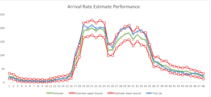
Figure 6 shows the estimation result of the arrival model with days clustered in type 4. For each period, we estimate a poison distribution. We draw the upper bound and lower bound of the 95% confidential interval of the estimated model in red lines. The green line (estimate) is the mean of 1000 runs of samples from the estimated distribution and it fits well as expected. The blue line is the mean of a test set where these days are randomly picked weekdays without significant damages reported. These test data are not from training data and are not used in model estimation. As one can see in Figure 6, the blue line mostly fits in the range of the 95% confidential interval of the estimated distributions.
This indicates that the estimation on arrival rate models is appropriate for us to use as estimation of arrival calls to the electricity company.
Figure 6. Arrival Rate Estimation
D. Simulation Result
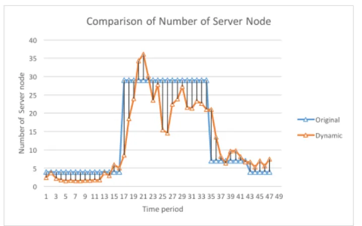
In this section, we report our simulation results using the arrival models. The electricity company also provides us its resource provision plan of the number of servers in each period. Figure 7 shows as the heuristics the deployed service nodes in each period. The heuristics has been adjusted to fit their demands in weekdays and is currently running in practice.
We use the estimated arrival model of type 4 to run simulation. We report the performance of the heuristics in Table III. As one can see, each period has around 19.2 servers deployed, and the simulation result shows that a customer on average waiting 1.6 minus to be served and the maximum length of the waiting queue is 17.
We run the simulation to compare the heuristics with the dynamic resource provision strategy. We set the strategy as the following: adding a new server whenever the queue length is more than 5 or the customer waiting time is more than 3 minutes. The required number of servers is shown in Figure 7 and the performance is shown in Table III for comparison. The result shows that by increasing the cost 5%(20.216-19.251/19.251, i.e., roughly increasing 0.965 server on average per period), the service quality can be improved by reducing the waiting time 13.8%(0.224/1.624) and the queuing length 47%(8/17).
Table III
PERFORMANCE BETWEEN THE HEURISTICS AND THE DYNAMIC RESOURCE PROVISION
Heuristic Dynamic Average number of server 19.251 20.216 Average waiting time 1.624 min 1.401 min
Maximum queue length 17 9
The ratio of customers waiting more
than >3mins 15.5% 10.25%
V. CONCLUSION
We propose a new cloud resource provision approach for time-varying demand services using simulation, unsupervised clustering and distribution estimation techniques. We cluster
Figure 7. Number of server nodes required in the heuristics and dynamic resource provision
days that have similar arrival patterns together to cater for time varying demands of services and adopt existing arrival rate modeling and estimation to observe formed distribution in presence of clustering. This helps cloud providers have an idea of how to provision their resources in an unpredictable environment with changing demands. By conducting the real case study, we show that compared to past heuristics adopted in real life, by adopting the dynamic allocation strategy, ser-vice providers can have a better reservation plan that improves their system performance with less resources allocated.
ACKNOWLEDGMENT
We thank anonymous reviewers for their valuable com-ments. This work was supported in part by Taiwan Information Security Center (TWISC), Academia Sinica, and Ministry of Science and Technology, Taiwan, under the grant MOST 104-2218-E-001-002 and MOST-103-2221-E-004 -006 -MY3.
REFERENCES
[1] R. Buyya, A. Beloglazov, and J. Abawajy, “Energy-efficient management of data center resources for cloud computing: a vision, architectural elements, and open challenges,” arXiv preprint arXiv:1006.0308, 2010. [2] P. Mell and T. Grance, “The nist definition of cloud computing,” 2011. [3] F. Yu, Y.-w. Wan, and R.-h. Tsaih, “Quantitative analysis of cloud-based streaming services,” in Services Computing (SCC), 2013 IEEE International Conference on, pp. 216–223, IEEE, 2013.
[4] S. Chaisiri, B.-S. Lee, and D. Niyato, “Optimization of resource provi-sioning cost in cloud computing,” Services Computing, IEEE Transac-tions on, vol. 5, no. 2, pp. 164–177, 2012.
[5] E. Amazon, “Amazon elastic compute cloud (amazon ec2),” Amazon Elastic Compute Cloud (Amazon EC2), 2010.
[6] R. N. Calheiros, M. A. Netto, C. A. De Rose, and R. Buyya, “Emusim: an integrated emulation and simulation environment for modeling, eval-uation, and validation of performance of cloud computing applications,” Software: Practice and Experience, vol. 43, no. 5, pp. 595–612, 2013. [7] B. N. Oreshkin, N. Regnard, and P. L’Ecuyer, “Rate-based daily arrival
process models with application to call centers,” tech. rep., Working Paper, Universit´e de Montr´eal, 2014.
[8] R. N. Calheiros, R. Ranjan, A. Beloglazov, C. A. De Rose, and R. Buyya, “Cloudsim: a toolkit for modeling and simulation of cloud computing environments and evaluation of resource provisioning algorithms,” Soft-ware: Practice and Experience, vol. 41, no. 1, pp. 23–50, 2011. [9] R. Buyya, R. Ranjan, and R. N. Calheiros, “Modeling and simulation
of scalable cloud computing environments and the cloudsim toolkit: Challenges and opportunities,” in High Performance Computing & Simulation, 2009. HPCS’09. International Conference on, pp. 1–11, IEEE, 2009.
[10] B. Wickremasinghe, R. N. Calheiros, and R. Buyya, “Cloudanalyst: A cloudsim-based visual modeller for analysing cloud computing envi-ronments and applications,” in Advanced Information Networking and Applications (AINA), 2010 24th IEEE International Conference on, pp. 446–452, IEEE, 2010.
[11] B. Wickremasinghe et al., “Cloudanalyst: A cloudsim-based tool for modelling and analysis of large scale cloud computing environments,” MEDC project report, vol. 22, no. 6, pp. 433–659, 2009.
[12] S. K. Garg and R. Buyya, “Networkcloudsim: Modelling parallel appli-cations in cloud simulations,” in Utility and Cloud Computing (UCC), 2011 Fourth IEEE International Conference on, pp. 105–113, IEEE, 2011.
[13] W. Zhao, Y. Peng, F. Xie, and Z. Dai, “Modeling and simulation of cloud computing: A review,” in Cloud Computing Congress (APCloudCC), 2012 IEEE Asia Pacific, pp. 20–24, IEEE, 2012.
[14] D. Kliazovich, P. Bouvry, and S. U. Khan, “Greencloud: a packet-level simulator of energy-aware cloud computing data centers,” The Journal of Supercomputing, vol. 62, no. 3, pp. 1263–1283, 2012.
[15] S.-H. Lim, B. Sharma, G. Nam, E. K. Kim, and C. R. Das, “Mdcsim: A multi-tier data center simulation, platform,” in Cluster Computing and Workshops, 2009. CLUSTER’09. IEEE International Conference on, pp. 1–9, IEEE, 2009.
[16] P. Jamshidi, A. Ahmad, and C. Pahl, “Autonomic resource provisioning for cloud-based software,” in Proceedings of the 9th International Symposium on Software Engineering for Adaptive and Self-Managing Systems, pp. 95–104, ACM, 2014.
[17] D. Kusic and N. Kandasamy, “Risk-aware limited lookahead control for dynamic resource provisioning in enterprise computing systems,” Cluster Computing, vol. 10, no. 4, pp. 395–408, 2007.
[18] H. C. Lim, S. Babu, and J. S. Chase, “Automated control for elastic stor-age,” in Proceedings of the 7th international conference on Autonomic computing, pp. 1–10, ACM, 2010.
[19] M. N. Bennani and D. A. Menasce, “Resource allocation for autonomic data centers using analytic performance models,” in Autonomic Comput-ing, 2005. ICAC 2005. Proceedings. Second International Conference on, pp. 229–240, IEEE, 2005.
[20] S. Chaisiri, B.-S. Lee, and D. Niyato, “Optimal virtual machine place-ment across multiple cloud providers,” in Services Computing Confer-ence, 2009. APSCC 2009. IEEE Asia-Pacific, pp. 103–110, IEEE, 2009. [21] S.-L. Chung, S. Lafortune, and F. Lin, “Limited lookahead policies in supervisory control of discrete event systems,” Automatic Control, IEEE Transactions on, vol. 37, no. 12, pp. 1921–1935, 1992.
[22] M. Arlitt and T. Jin, “A workload characterization study of the 1998 world cup web site,” Network, IEEE, vol. 14, no. 3, pp. 30–37, 2000. [23] H. Zhang, G. Jiang, K. Yoshihira, H. Chen, and A. Saxena, “Intelligent
workload factoring for a hybrid cloud computing model,” in Services-I, 2009 World Conference on, pp. 701–708, IEEE, 2009.
[24] “U.S. Viewers Watched an Average of 3 Hours of Online Video in July - comScore, Inc.” http://www.comscore.com/Insights/Press-Releases/ 2007/09/US-Online-Video-Streaming. (Accessed on 03/06/2016). [25] A. N. Avramidis and P. L’Ecuyer, “Modeling and simulation of call
centers,” in Simulation Conference, 2005 Proceedings of the Winter, pp. 9–pp, IEEE, 2005.
[26] N. Roy, A. Dubey, and A. Gokhale, “Efficient autoscaling in the cloud using predictive models for workload forecasting,” in Cloud Computing (CLOUD), 2011 IEEE International Conference on, pp. 500–507, IEEE, 2011.
[27] I. Cunha, J. Almeida, V. Almeida, and M. Santos, “Self-adaptive capac-ity management for multi-tier virtualized environments,” in Integrated Network Management, 2007. IM’07. 10th IFIP/IEEE International Sym-posium on, pp. 129–138, IEEE, 2007.
[28] J. A. Hartigan and M. A. Wong, “Algorithm as 136: A k-means clustering algorithm,” Journal of the Royal Statistical Society. Series C (Applied Statistics), vol. 28, no. 1, pp. 100–108, 1979.
[29] X. Meng, J. Bradley, B. Yavuz, E. Sparks, S. Venkataraman, D. Liu, J. Freeman, D. Tsai, M. Amde, S. Owen, et al., “Mllib: Machine learning in apache spark,” arXiv preprint arXiv:1505.06807, 2015.
[30] “Mllib — apache spark.” http://spark.apache.org/mllib/. (Accessed on 03/06/2016).
[31] E. Buist and P. L’Ecuyer, “A java library for simulating contact centers,” in Proceedings of the 37th conference on Winter simulation, pp. 556– 565, Winter Simulation Conference, 2005.