國 立 交 通 大 學
電 信 工 程 學 系 碩 士 班
碩 士 論 文
針對埠或位址掃描做快速偵測之
適應性接續假設測試
Adaptive Sequential Hypothesis Testing for Fast
Detection of Port/Address Scan
研究生:林建成
指導教授:李程輝 教授
針對埠或位址掃描做快速偵測之適應性接續假設測試
Adaptive Sequential Hypothesis Testing for Fast Detection of
Port/Address Scan
研究生:林建成 Student: Jian-Cheng Lin
指導教授:李程輝 教授 Advisor: Prof. Tsern-Huei Lee
國 立 交 通 大 學
電 信 工 程 學 系 碩 士 班
碩 士 論 文
A Thesis
Submitted to Institute of Communication Engineering Collage of Electrical Engineering and Computer Science
National Chiao Tung University in Partial Fulfillment of Requirements
for the Degree of Master of Science
in
Communication Engineering July 2007
Hsinchu, Taiwan, Republic of China
針對埠或位址掃描做快速偵測之
適應性接續假設測試
學生:林建成
指導教授:李程輝 教授
國立交通大學
電信工程學系碩士班
中文摘要
隨著網路應用服務的增加,網路安全的議題也越來越受到廣泛的重視。其中 埠或位址掃描這種異常的行為,是網路入侵的一個重要途徑。早期偵測這些埠或 位址掃描的技術,是建立於惡意行為的主機具有較高掃描率的基礎上。但是這種 方式對於偵測某些慢速的掃描並不適用,而且攻擊者一旦獲知發出警戒的門檻 值,便能輕易的躲過這種偵測。為了解決這個問題,接續假設性測試便成為偵測 這種掃描的另一種替代方案。這種方式可以藉由第一次連線要求的成功率之不 同,來判斷發送者為正常或具有惡意攻擊行為的主機。但是假如無法知道正常與 異常主機不同的連線成功率為何,其誤判的機率便會遠高於理想值。在這篇碩士 論文中,我們比較了幾種以接續假設性測試為架構的技術,並且發現在實際未知 連線成功率的網路中,這些基本的接續假設性測試並不適用。因此,我們提出在 此測試法的基礎架構上,加入了一個簡單的適應性演算法,可以準確的估計出這 些機率值。而從模擬的結果也顯示出,這個適應性的估計演算法對於原本的接續 假設性測試法有極大的改善,因為它使原本對於埠或位址掃描的測試法更加健全 與完備。Adaptive Sequential Hypothesis Testing for Fast
Detection of Port/Address Scan
Student: Jian-Cheng Lin
Advisor: Prof. Tsern-Huei Lee
Institute of Communication Engineering
National Chiao Tung University
Abstract
As more and more network applications and services are provided, the topic of network security becomes more and more important. The behavior anomaly of port/address scans is a way to intrude hosts on the Internet. Early detection techniques of port/address scans are based on the observation that malicious hosts could send scans with high scanning rates. But such approaches are not suitable to detect scanners with lower scanning rate. Once the threshold of scanning rate for generating alerts is known to the attackers, the detection will be easily evaded. In order to overcome the problems, sequential hypothesis testing is an alternative detection technique. According to the probabilities of success for the first-contact connection attempts sent by the hosts, sequential hypothesis testing can detect the senders as benign or malicious. If these probabilities are unknown, the false positive and false negative rates could be much larger than the desired values. In this thesis, we compare several techniques based on sequential hypothesis testing and realize these techniques inadequate for a real network. Therefore, we propose a simple adaptive algorithm which provides accurate estimation of these probabilities. Simulation results show that the proposed adaptive estimation algorithm provides a great improvement for sequential hypothesis testing.
致謝
首先,要感謝我的指導教授─李程輝老師,在我研究所的求學過程中悉心地 指導與教誨,並且適時的給予實用的建議與鼓勵。從老師的身上,我看到了一位 真正的學者對於研究的認真態度與無比熱忱,這是讓我由衷地欽佩和感動的。在 老師的指導下,讓我初窺到學術殿堂的門徑,也讓我學習到做研究應有的態度與 方法,實在是獲益良多。 感謝 NTL 實驗室的所有夥伴們,這兩年來的朝夕相處,讓我感受到無比的 溫暖。謝謝景融、郁文、迺倫、以及瑋哥,眾位學長姐的關心與照顧讓我感念在 心;謝謝嘉旂、柏庚、和登煌,這些日子一起修課一起通霄熬夜的革命情感令我 難以忘懷;謝謝北極、耀誼、世弘、明鑫、凱文、西西搭,你們這群可愛的學弟 們,讓我的碩士生涯過得很愉快,也充滿了各種美好的回憶。 最後,更要感謝我的父母與其他親人好友們,謝謝你們永遠給我無限的支持 與鼓勵,讓我有信心有勇氣去面對各種挑戰。因為有你們,是讓我不斷向前邁進 的原動力! 謹將此論文獻給所有愛我與我愛的人 2007 年 7 月 新竹交大Contents
Contents
中文摘要 ... i English Abstract ... ii 誌謝 ... iii Contents ... iv List of Tables ... viList of Figures ... vii
Chapter 1 Introduction ... 1
Chapter 2 Background ... 5
2.1 Scanning Worms ... 5
2.2 Scan Detection and Suppression ... 7
2.3 False Alarm ... 9
2.3.1 False Positive & False Negative ... 9
2.3.2 Probabilities ... 10
Chapter 3 Related Works ... 11
3.1 First-Contact Connection Requests ... 11
3.2 Sequential Hypothesis Testing ... 13
3.2.1 Model ... 13
3.2.2 Upper and Lower Thresholds ... 16
Contents
3.2.4 Number of Observations to Select Hypothesis ... 18
3.3 Simplified Sequential Hypothesis Testing ... 19
3.3.1 Modification from SHT ... 20
3.3.2 Hardware Implementation ... 20
3.3.3 Algorithm ... 22
3.4 Reverse Sequential Hypothesis Testing ... 23
3.4.1 Model ... 24
3.4.2 Proof of Optimized Algorithm ... 25
3.4.3 Log of Likelihood Ratio ... 27
Chapter 4 Adaptive Sequential Hypothesis Testing ... 29
4.1 Scheme 1 ... 29
4.2 Scheme 2 ... 33
4.3 Implementation ... 34
Chapter 5 Simulation Results ... 38
5.1 SHT with known θ0 and θ1 ... 38
5.2 SHT with unknown θ0 and θ1 ... 45
5.3 Adaptive Sequential Hypothesis Testing ... 48
Chapter 6 Conclusion ... 54
List of Tables
List of Tables
Table 2.1 Definition of false positive and false negative... 9
Table 2.2 Example of false positive and false negative ... 10
Table 5.1 The step sizes of failure and success for SHT... 41
Table 5.2 SHT, θ0 and θ1 are known ... 42
Table 5.3 Simplified SHT, θ0 and θ1 are known ... 43
Table 5.4 RSHT, θ0 and θ1 are known ... 44
Table 5.5 SHT, θ0 and θ1 unknown, guess 0.8 and 0.2 ... 46
Table 5.6 RSHT, θ0 and θ1 unknown, guess 0.8 and 0.2... 47
Table 5.8 Adaptive SHT, NG ≥0 & NB ≥0 (0%)... 49
Table 5.9 Adaptive SHT, NG ≥200 & NB ≥50 (25%) ... 50
Table 5.10 Adaptive SHT, 320≤NG ≤480 & 80≤NB ≤120 (40~60%) ... 51
Table 5.11 Adaptive SHT, NG:NB (40~60%) ... 52
List of Figures
List of Figures
Figure 2.1 Spreading and propagation of scanning worms... 6
Figure 2.2 Preventing “inside” from “outside”... 8
Figure 3.1 X , the outcomes of FCC requests from r to li i ... 12
Figure 3.2 Flow diagram of sequential hypothesis testing ... 15
Figure 3.3 A log scale graph of Λ X
( )
n for SHT ... 16Figure 3.4 Connection cache... 21
Figure 3.5 Address cache ... 22
Figure 3.6 Algorithm for the simplified SHT ... 22
Figure 3.7 A log scale graph tracing the value of Λ X
( )
n for SHT... 24Figure 3.8 A log scale graph tracing the value of Λ X for RSHT... 24
( )
n Figure 4.1 Adaptive procedure I ... 32Figure 4.2 Adaptive procedure II... 34
Figure 4.3 List of connection ... 35
Figure 4.4 Connection Table ... 35
Figure 4.5 Address Table ... 36
Chapter 1 Introduction
Chapter 1
Introduction
As the computer and network technologies advance rapidly, more and more services and applications are provided on the Internet. Today, many people can’t live without computers and networks. Therefore the topic of network security becomes more and more important.
As time goes by, modern computer worms and viruses can spread at a speed much faster than human intervention. A computer worm automatically spreads from computer to computer by exploiting a software vulnerability that allows an arbitrary program to be executed without proper authorization. In recent years, people discovered many kinds of worms, such as the Code Red [11], Nimda [12], and Slammer [6], which infected thousands upon thousands of computers on the Internet in a short period of time and caused great damage to our society. It’s important to prevent the majority of vulnerable systems from being detected and minimize the damage caused by computer worms. Fast and accurate detection of worms when they are spreading is, therefore, helpful to solve the problems.
Chapter 1 Introduction
categories – protocol analysis, pattern matching, and behavior anomaly. First, protocol analysis is used to inspect if there are misused protocol fields in the header of a packet. The header of a packet sent by a malicious host is usually spoofed or altered. The malicious hosts can be detected according to the misuse of fields. Then, pattern matching is used to look for specific patterns in the payload of a packet or across packets. The signatures of worms, e.g. specific unique patterns or strings of malicious codes, can be extracted and then utilized for worm detection. Although pattern matching is accurate, it is limited to detect worms with identified signatures. If the signatures of new worms are not created promptly, the majority of vulnerable systems could be infected.
Finally, behavior anomaly can be used to detect and prevent port/address scans because an infected host is likely to behave differently from a normal host. For example, an infected host could try to infect other vulnerable host on the Internet with port or address scanning. Therefore, we can detect the infected host with the observation that it has high new connection attempt rate or high failure rate of new connection attempts. Because the technique based on behavior anomaly can detect worms without signatures, it is useful to deal with new computer worms.
Seeing that most of current intrusion detection systems (IDS) based on the technique of pattern matching can’t detect new and unknown malicious attacks or scans, network behavior anomaly detection (NBAD) is receiving more and more attention. Recently, more and more IDS adopted the mechanism based on behavior anomaly detection. For example, the Network Security Monitor (NSM) [13] and Snort [14] are designed according to simple observation of high scanning rate by an infected host.
Chapter 1 Introduction
In the paper [1], a technique of sequential hypothesis testing for scan detection is proposed, and the algorithm is called Threshold Random Walk. The technique is based on the observation that success rate of a connection attempt sent by a malicious host is much lower than the success rate of a connection attempt sent by a benign host. A random walk of each host is moving upward if a connection attempt is a failure, or moving downward if a connection attempt is a success. A host is detected as malicious if the position of its random walk is greater than the upper threshold or as benign if it is smaller than the lower threshold. A simplified sequential hypothesis testing [3] is suitable for both software and hardware implementations. It modified the step sizes of moving upward and downward to be identical. The reverse sequential hypothesis testing [2] can detect malicious host slightly faster than the original algorithm. The three algorithms will be review in Chapter 3.
The sequential hypothesis testing assumes that the success rates of connection attempts sent by benign and malicious hosts are known. They are used to compute the step sizes of moving upward and downward. But in fact, the success rates of connection attempts could be unknown. Therefore, we develop the sequential hypothesis testing with an adaptive procedure which can estimate the success rates of connection attempts based on their outcomes. It can provide estimates close to real values and reduce both the false positive and negative rates
The rest of this thesis is organized as follows. In Chapter 2, we introduce some background about scanning worms, scan detection and suppression, and the definition of false positives and false negatives. In Chapter 3, we review the sequential hypothesis testing, the simplified sequential hypothesis testing, and
Chapter 1 Introduction
reverse sequential hypothesis testing. In Chapter 4, we present our proposed adaptive algorithm for estimation of success rate of connection attempts. Simulation results are provided in Chapter 5. Finally, we draw conclusion in Chapter 6.
Chapter 2 Background
Chapter 2
Background
2.1
Scanning Worms
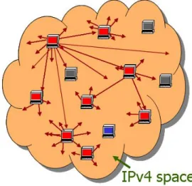
A computer worm is a form of malware that spreads from host to host without human intervention. A scanning worm locates vulnerable hosts by generating a list of addresses to probe and then contact them. Figure 2.1 illustrates that worms can self-propagate among the hosts exploiting security or policy flaws in widely-used services [10]. An infected host initiates scans and infects the other benign hosts. Subsequently, the benign hosts become infected ones and then join the army of scanning. Finally all the hosts on the Internet will be infected.
This addresses list may be generated sequentially or pseudo-randomly. Local addresses are often preferentially selected because the communication between neighboring hosts will likely encounter fewer defenses [5]. Scans may take the form of TCP connection requests (SYN packets) or UDP packets. In the case of the connectionless UDP protocol, it is possible for the scanning packet to also contain the body of the worm, such as the Slammer worms [6].
Chapter 2 Background
Figure 2.1 Spreading and propagation of scanning worms
Scanning worms probe attempts to determine if a service is operating at a target IP address and then discover new victims. They have two basic scanning types – horizontal scans, which look for an identical service on a large number of hosts, and vertical scans, which examine an individual host to discover all running services.
There are many kinds of techniques to generate a list of addresses for scanning worms, such as linear scanning of an IP address space (Blaster), fully random (Code Red), a bias toward local address (Code Red II and Nimda), or even more enhanced techniques (Permutation Scanning). While more and more scanning worms change their style of scanning to avoid being detected, all of they still have two common properties as follows. Most of the scanning attempts may result in failure, and the infected hosts will send many connection attempts [4]. As long as we look for a class of behavior rather than specific worm signatures, most new worms will be detected.
In the next chapter, we will introduce three kinds of existing on-line algorithms to detect the presence of scanning worms by observing network traffic. These
Chapter 2 Background
infected hosts and normal hosts according to the success rate of connection attempts.
2.2
Scan Detection and Suppression
Human reaction time is inadequate for detecting and responding to fast scanning worms, such as Slammer, which can infect the majority of vulnerable hosts on the entire IP address space in a few minutes [6, 7]. Thus, today’s worm detection techniques focus on automated response to worms, such as quarantining infected machines, automatic generation and installation of patches, and reducing the rate at which worms can send connection attempts [8].
But, an automated response will be of little use if it fails to be triggered quickly after a host is infected. Infected hosts with high network bandwidth can send thousands of connection attempts per second, each of which has the potential to spread the infection. On the other hand, an automated response that triggers too easily will erroneously identify normal hosts as infected. It will interfere with the normal activity of these hosts and cause significant damage.
Many scan detection mechanisms rely on the observation that only a small part of addresses are likely to respond to a connection attempt at any given port. If a connection attempt is sent to an inactive host, it will also be failed. When a connection attempt does reach an active host, it would be rejected possibly because not all hosts will be running the targeted services. Thus, the infected hosts are likely to have a low rate of successful connection attempts, whereas benign hosts, which only send connection attempts when there is reason to believe that addresses will
Chapter 2 Background
respond, will have a higher success rate. So, we can make good use of the properties described above to detect scanning worms with malicious connection attempts.
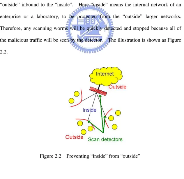
Worm containment is designed to stop the spread of worms in a local area network or an enterprise by detecting infected machines and preventing them from contacting other systems. Current approaches to containment are base on detecting the scanning activity, and the key component for today’s containment techniques is scan suppression which responds to detected infected hosts by blocking future scanning attempts. [4]
The goal of scan suppression is to prevent scanning attempts coming from “outside” inbound to the “inside”. Here “inside” means the internal network of an enterprise or a laboratory, to be protected from the “outside” larger networks. Therefore, any scanning worms will be quickly detected and stopped because all of the malicious traffic will be seen by the detector. The illustration is shown as Figure 2.2.
Chapter 2 Background
2.3
False Alarm
When the scan detection mechanisms determine a host is malicious or benign, it is possible to make error decisions, such as regarding as malicious when the host is benign or regarding as benign when it is infected actually. Both of them are called false alarm. We hope that the scan detection mechanism would distinguish between malicious and benign hosts as precisely as possible, and the probability of false alarm is as less as possible. So, we can use false alarm rate to judge whether an algorithm is suitable for scan detection.
2.3.1
False Positive & False Negative
The false alarm can be divided into two conditions which are false positive and false negative [9]. The former is the error of rejecting something that should have been accepted, such as finding an innocent host guilty. The latter is the error of accepting something that should have been rejected, such as finding a guilty host innocent. Table 2.1 and 2.2 will illustrate these conditions as follows.
Actual Condition
Present Absent Positive Condition Present + Positive Result
= True Positive
Condition Absent + Positive Result = False Positive Test
Result
Negative Condition Present + Negative Result = False Negative
Condition Absent + Negative Result = True Negative Table 2.1 Definition of false positive and false negative
Chapter 2 Background
Actual Condition
Scanner Benign Scanner Actual Scanner + Result Scanner
= Detection
Actual Benign + Result Scanner = False Positive Test
Result
Benign Actual Scanner + Result Benign = False Negative
Actual Benign + Result Benign = Normal
Table 2.2 Example of false positive and false negative
2.3.2 Probabilities
The false positive rate is the proportion of negative instance that were erroneously reported as being positive. The false negative rate is the proportion of positive instance that were erroneously reported as being negative. So we can define them as follows.
number of false positives false positive rate =
number of negative instances number of false negatives false negative rate =
number of positive instances
For scan detection, we can also define four outcomes as follow.
FP
number of scanner but actually benign
false positive rate = P
number of total benign =
FN
number of benign but actually scanner
false negative rate = P
number of total scanner =
1
NM FP
number of benign and actually benign
normal rate = P P
number of total benign = = −
1
DT F
number of scanner and actually scanner
detection rate = P P
Chapter 3 Related Works
Chapter 3
Related Works
3.1
First-Contact Connection Requests
In the previous chapter, we can know that one of the main characteristics of infected hosts is that they are more likely to choose hosts that do not exist or do not have the requested service activated than benign hosts. This is because they lack precise knowledge of which hosts and ports are currently active.
Using this observation, there are several kinds of on-line algorithms to detect malicious attacks or connection attempts. The goal of these approaches is to reduce the number of observed connection attempts to flag malicious hosts, while bounding the probabilities of false positive and false negative.
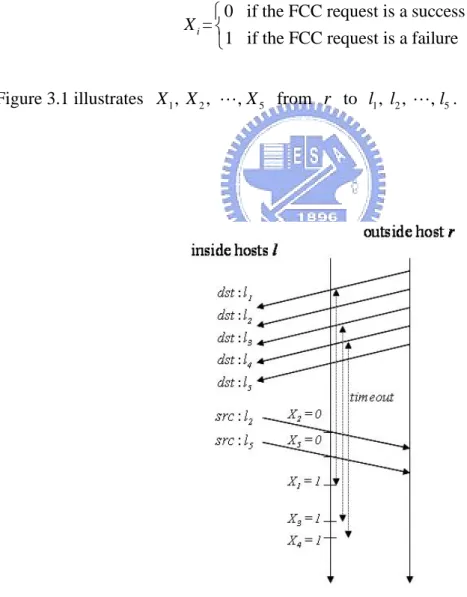
An event is generated and monitored when a remote source r makes a first-contact connection (FCC) request to a local destination l. An FCC request is a connection request which is addressed to a host the sender has not previous communicated. These events are monitored because malicious scans are mostly composed of first-contact connection requests.
Chapter 3 Related Works
Only the TCP connections are considered and thus a TCP SYN packet indicates a connection request. The outcome of an FCC request is classified as either a “success” or a “failure”. It is a success if the host l replies a SYN-ACK packet or a failure if host l replies a RST packet or does not reply at all. If the request sent by r is a UDP packet, any UDP packet from l received before the timeout will be a success.
For a given remote (outside) host r, let X be a random variable that represents i the outcome of the FCC request from r to the ith distinct local (inside) host li, where
0 if the FCC request is a success =
1 if the FCC request is a failure
i
X ⎧⎨ ⎩
Figure 3.1 illustrates X1, , , X2 " X from to 5 r l1, , , l2 " l5.
Chapter 3 Related Works
The outcomes X , 1 X , …, are observed so that host r can be determined to be 2 either malicious or benign. Undoubtedly, we would like to make this detection as quickly and correctly as possible. The method of sequential hypothesis testing (SHT) developed by Wald [1] is suitable for scanning worm detection. In the following sections, several techniques based on SHT will be introduced.
3.2
Sequential Hypothesis Testing
3.2.1 Model
In the paper [2], the technique of sequential hypothesis testing is developed. The algorithm is called Threshold Random Walk (TRW). There are two hypotheses:
, where is the null hypothesis that the remote host r is benign and is the hypothesis that r is malicious.
0 and
H H1 H0 H1
To simplify the analysis, it is assume that, conditioning on hypothesis H , the j random variables X1|H , j X2|H , … are independent and identically distributed j (i.i.d) with probability mass function
[
]
[
]
[
]
[
]
0 0 0 1 1 1 1 P 0 | P 1| 1 P 0 | P 1| 1 i i i i X H X H X H X H 0 θ θ θ θ = = = = − = = = = −For some θ0 and θ1 which satisfy θ0 > . It is because a FCC attempts is more θ1 likely to be a success from a benign host than a malicious host.
Chapter 3 Related Works
Given the two hypothesis, there are four possible decisions as follows. The decision is called a detection when the algorithm selects when is in fact true. On the other hand, it is called a false negative if the algorithm chooses . Likewise, when is in fact true, selecting constitutes a false positive and selecting when is called a normal. These four possible outcomes are represented as: 1 H H1 0 H 0 H H1 0 H H0
[
]
[
]
[
]
[
]
1 1 0 1 1 0 0 0 : P choose | is true : P choose | is true 1 : P choose | is true : P choose | is true 1 DT FN DT FP NM FP Detection H H P False Negative H H P P False Positive H H P Normal H H P P = = = − = = = −The desired performance of the TRW algorithm can be specified with the detection probability PDT and the false positive probability PFP . Let α represents the upper bound of false positive probability and β denote the lower bound of detection probability. In other word, we desire
and
FP DT
P ≤α P ≥ β where typical values might be α =0.01 and β =0.99.
As the outcome of X is observed, we calculate the likelihood ratio: i
( )
[
[
1]
]
[
[
1]
]
1 0 1 P | P | P | P | n n i n i n i H X H = X Λ X ≡ X =∏
X H H)
nChapter 3 Related Works
Note that Λ X
( )
n can be updated incrementally. Let φ( )
Xi represent the likelihood ratio of the ith observation. It holds that( )
( ) (
1) ( )
( )
0 1 , 1 n n i n n i X X φ − φ = Λ X =∏
=Λ X Λ X =( )
[
[
]
]
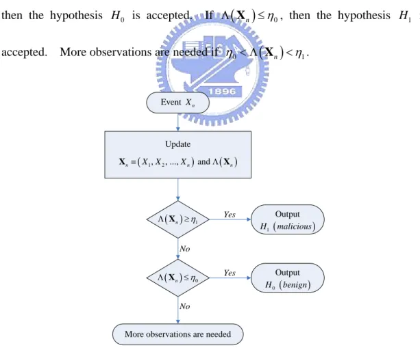
10 1 0 1 1 1 0 1 if 1 (failure) P | P | 1 if 0 (success) i i i i i X X H X X H X θ θ θ θ φ − − ⎧ > = ⎪ ≡ = ⎨ < = ⎪⎩The flow diagram is shown in Figure 3.2. The updated likelihood ratio is compared to an upper threshold
( )
nΛ X
1
η and a lower threshold η0. If Λ
( )
Xn ≥η1,then the hypothesis H0 is accepted. If Λ
( )
Xn ≤η0, then the hypothesis isaccepted. More observations are needed if
1
H
( )
0 n 1
η < Λ X <η .
More observations are needed Update ( 1, 2, ..., ) and ( ) n≡ X X Xn Λ n X X Event Xn ( )n η1 Λ X ≥ ( )n η0 Λ X ≤ Output ( ) 0 H benign Output ( ) 1 H malicious Yes Yes No No
Chapter 3 Related Works
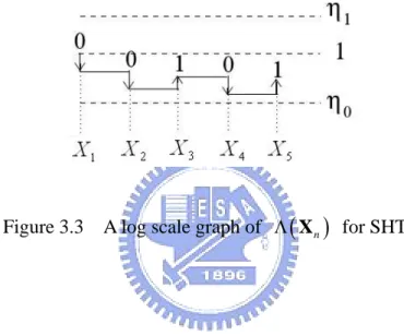
Figure 3.3 represents a log scale graph of Λ X
( )
n when each observation X iis added to the sequence. Each success (0) observation decreases , moving it closer to the benign conclusion threshold
(
nΛ X
)
0
η . Each failure (1) observation increases , moving it closer to the infection conclusion threshold
(
nΛ X
)
η1.Figure 3.3 A log scale graph of Λ X
( )
n for SHT3.2.2
Upper and Lower Thresholds
To develop the algorithm described in the previous section, the thresholds
0 and 1
η η can be bounded by simple expressions of PFP and PDT [1].
Consider a sample path of observations X X1, , 2 ..., X . The upper threshold n
1
η is hit on the observation X and hypothesis n H1 is selected. Thus,
( )
[
[
1 2 1]
]
1 1 2 0 P , , ..., | P , , ..., | n DT n n FP X X X H P X X X H P η Λ X ≡ = ≥Chapter 3 Related Works
DT
P , and the second ( is selected when is true) is the false positive probability .
1
H H0
FP
P
Similarly, if the lower threshold η0 is hit and hypothesis H0 is selected, then
( )
[
[
1 2 1]
]
0 1 2 0 P , , ..., | 1 P , , ..., | 1 n DT n n FP X X X H P X X X H P η − Λ ≡ = ≤ − XTherefore, the upper and lower bounds can be bounded in terms of PFP and PDT.
1 0 1 and 1 DT D FP FP P P P P η ≤ η ≥ − T −
In real implementation, one can use the approximations PFP =α , PDT = and set β
1 0 1 and 1 β β η η α α − = = −
3.2.3
Log of Likelihood Ratio
Moreover, one can use the log-likelihood ratio to simplify computation. It can be formulated as follows.
( )
(
)
[
]
[
]
(
( )
)
( )
(
)
( )
(
)
1 0 1 1 0 1 1 0 0 , 0 1 1 0 if 1 P | 0 if 0 P | n n n i n n i i i i i i i S ln Y S Y S ln ln F X X H Y ln ln X ln ln S X X H θ θ φ θ θ − = ≡ Λ = = + = ⎛ ⎞ ⎧⎪ − − − ≡ > = ≡ ⎜⎜ ⎟⎟= =⎨ − ≡ < = ⎪⎩ ⎝ ⎠∑
XChapter 3 Related Works
lower threshold ln
( )
η0 . If Sn ≥ln( )
η1 , then the hypothesis H0 is accepted. If( )
0n
S ≤ln η , then the hypothesis H1 is accepted. More observations are needed if
( )
0 n( )
1 ln η <S <ln η .3.2.4
Number of Observations to Select Hypothesis
In this section, the average number of FCC attempts sent by a remote host to detect it as benign or malicious is calculated. The smaller the number of observations, the faster a remote host will be identified.
N
For the analysis of , the log of likelihood ratio should be used. Because is the summation of random variables where is also a random variable, the expected value of equals to the product of expected values of and .
N SN N Yi N N S Yi N
[ ]
[ ] [ ]
1 2 N N N S = + + +Y Y " Y ⇒ E S =E Y E Ni 1 HTherefore, we can derive expressions for the expected values of and , conditioning on hypotheses . The conditional expected value of is the ratio of the conditional expected values of and .
N S Yi 0 and H N N S Yi For Yi,
( )
( )
( )
( )
1 0 1 0 1 0 1 0 1 0 1 0 0 1 1 1 1 1 with prob. 1 | with prob. with prob. 1 | with prob. i i ln Y H ln ln Y H ln θ θ θ θ θ θ θ θ θ θ θ θ − − − − ⎧ − ⎪ = ⎨ ⎪⎩ ⎧ − ⎪ = ⎨ ⎪⎩ ⇒[
]
(
)
( )
( )
[
]
(
)
( )
( )
1 1 0 0 1 1 0 0 1 0 0 1 0 1 1 1 1 1 | 1 | 1 i i E Y H ln ln E Y H ln ln θ θ θ θ θ θ θ θ θ θ θ θ − − − − = − + = − +Chapter 3 Related Works For SN,
( )
( )
( )
( )
1 0 0 1 1 0 with prob. | with prob. 1 with prob. | with prob. 1 N N ln S H ln ln S H ln η α η α η β η β ⎧⎪ = ⎨ − ⎪⎩ ⎧⎪ = ⎨ − ⎪⎩ ⇒[
]
( ) (
) ( )
[
]
( ) (
) ( )
0 1 1 1 | 1 | 1 N N E S H ln ln E S H ln ln 0 0 α η α η β η β η = + − = + −So, the conditional expected values of N : E N
[ ]
=E S[ ] [ ]
N E Yi[
]
(
( ) (
)
( )
) ( )
( )
[
]
( ) (
) ( )
(
)
( )
( )
1 1 0 0 1 1 0 0 1 0 0 1 0 1 0 1 0 1 1 1 1 1 1 | 1 1 | 1 ln ln E N H ln ln ln ln E N H ln ln θ θ θ θ θ θ θ θ α η α η θ θ β η β η θ θ − − − − + − = − + + − = − +It represents that the expected values of N varies with the parameters α , β, θ0, and θ1. With α =0.01, β =0.99, θ0 =0.8, and θ1=0.2, the expected values of
conditioning on hypotheses are both 5.41.
N H0 and H1
3.3
Simplified Sequential Hypothesis Testing
The huge complexity of monitoring FCC attempts of all remote hosts makes the TRW algorithm infeasible. In the paper [4], a simplified version of sequential hypothesis testing sets both the step sizes of moving upward and downward to one for the detection algorithm, and uses one bit to indicate whether or not host r has sent any connection to host l and another bit for the opposite direction. Each connection is recorded and indexed by hash the local IP address, remote IP address, and local port number for TCP protocol. A hash function is adopted to index the connections and reduce the space requirement.
Chapter 3 Related Works
3.3.1
Modifications from SHT
Using sequential hypothesis testing, each remote host has a likelihood value that a series of FCC requests from the given host reflect benign or malicious, based on how far the random walk deviates above or below the origin. The likelihood values of remote hosts are updated continuously when a FCC request is determined as a success or a failure. A successful connection request drives a random walk downward, whereas a failed connection request drives it upward.
The step sizes of moving upward and downward are both simplified to one. The likelihood value of each remote host is renamed as count representing the score of danger. If a successful FCC request is received, the score is added by 1. Oppositely, it is subtracted by 1 if a failure is received.
3.3.2 Hardware
Implementation
To implement TRW, we must track the establishment of FCC requests. It only considers the success or failure of connection attempts to new addresses. This approach inevitably requires a very large amount of state to keep track of which pairs of addresses have already tried to connect. When designing hardware, we often must store information in a fixed volume of memory. Since the information we would like to store may exceed this volume, one approach is to use approximate caches for which collisions will cause imperfections.
Chapter 3 Related Works
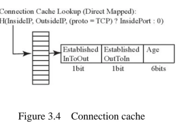
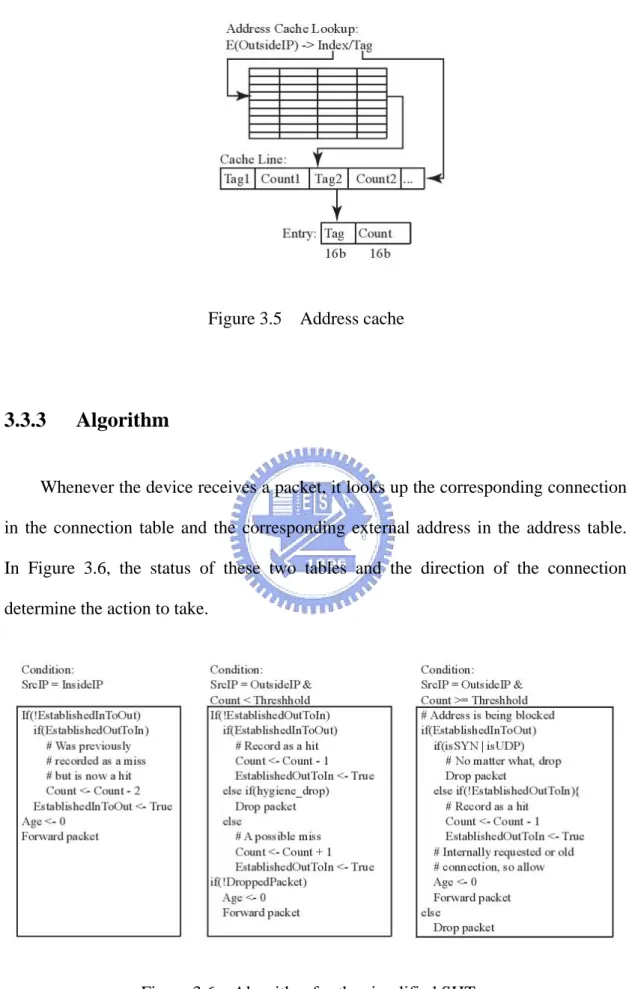
The scan detection and suppression algorithm approximates TRW in the following ways. The connections and addresses must be recorded using approximate caches. Figure 3.4 and 3.5 gives the overall data structures of the hardware implementation.
In Figure 3.4, connections are tracked using a fixed-sized table indexing by hashing the “inside” IP address, the “outside” IP address, and the inside port number for TCP. Each record consists of a 6-bit age counter and 1-bit field for each direction (connections from inside to outside and from outside to inside), recording whether a connection has been established in that direction.
Figure 3.4 Connection cache
In Figure 3.5, external (outside) addresses are also tracked by an associative approximate cache. To find an entry, the external IP addresses are encrypted by a 32-bit block cipher. The resulting 32-bit number will be separated into an index and a tag. The index is used to find the line of entries. The “count” tracks the score of danger (add 1 when the connection is a failure and subtract 1 when it is successful).
Chapter 3 Related Works
Figure 3.5 Address cache
3.3.3 Algorithm
Whenever the device receives a packet, it looks up the corresponding connection in the connection table and the corresponding external address in the address table. In Figure 3.6, the status of these two tables and the direction of the connection determine the action to take.
Chapter 3 Related Works
At first, consider the middle column of Figure 3.6. For a connection from a non-blocked outside IP address (count<threshold), reduce “age” to 0 and forward the packet if a corresponding connection has already been established in the packet’s direction. Otherwise, if the packet from the outside has been seen from the inside, forward the packet and decrement the address’s count by 1, as the outside address with a successful connection is credited. Otherwise, forward the packet but increment the address’s count by 1, as the address has one more outstanding, so-far unacknowledged connection request.
Likewise, for packets from inside addresses (the left column in Figure 3.6), if there is a connection establishment from the other direction, the count is reduced by 2 for compensation. This is because that the connection has been regarded as a failure previously and the count is added by 1.
Finally, consider the right column in Figure 3.6. If , the device blocks it. When receiving subsequent packet from that address, the action depends on the packet’s type and whether it matches an existing and successfully established connection. If the packet does not match an existing connection, we drop it. If it does, then we will still drop it if it’s a UDP packet or a TCP initial SYN. Otherwise, we allow it through.
count≥threshold
3.4
Reverse Sequential Hypothesis Testing
In the SHT, a host would no longer be observed when it was determined to be benign. In contrast, a scheme that concerned with detecting infection events is
Chapter 3 Related Works
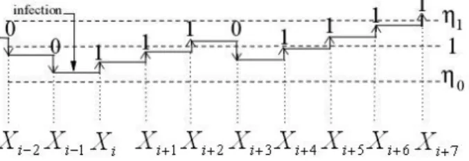
proposed in the paper [3]. It is possible that a remote host is infected when its likelihood ratio is close to but larger than η0, as shown in Figure 3.7. In this case, it takes more observations for the SHT algorithm to declare it to be malicious than doing so for a host which is infected when its likelihood ratio is equal to 1.
Figure 3.7 A log scale graph tracing the value of Λ X
( )
n for SHT3.4.1 Model
The solution to this problem is to run a new sequential hypothesis testing and evaluate the likelihood ratio in reverse chronological order when each connection is observed, as illustrated in Figure 3.8. To detect a host infected before but after , the reverse sequential hypothesis testing (RSHT) computes the likelihood ratio for the reversed vector of outcomes
i Y 1 i Y−
(
, ..., 1)
n ≡ Xn XX observed so far. Because
the most recent observations are process first, the RSHT will terminate before reaching the observations that were collected before infection.
Chapter 3 Related Works
A naïve implementation of repeated reverse sequential hypothesis testing requires storing an arbitrarily large sequence of FCC observation. In fact, there exists an iterative function with state variable Λ X to optimize the computation.
( )
n( )
n max(
1,(
n−1) ( )
φ Xn)
,( )
0 1Λ X = Λ X Λ X ≡
It can be calculate in sequence when events are observed and maintain the likelihood ratio larger than one. Because Λ X is updated in sequence, the
( )
nobservations can be discarded immediately after they are used to update Λ X .
( )
n3.4.2
Proof of Optimized Algorithm
The RSHT has the property that the likelihood value Λ X of optimized
( )
ncomputation exceed η1 if and only if the RSHT starting backward from observation n concludes that the host was infected.
( )
n η1(
Xn, Xn-1, , Xm)
η1 , m[ ]
1, nΛ X ≥ ⇔ Λ " ≥ ∈ #
We first prove the following lemma starting if the RSHT reports an infection, the optimized algorithm will also report an infection.
Lemma 1:
[ ]
(
)
( )
1 1 1 1 , m : , , , i n n-1 m nFor and for mutually independent random variables X
1, n X X X
η
η η
>
Chapter 3 Related Works
Proof:
We begin by replacing the Λ term with its equivalent expression in terms of φ.
(
)
1 , , , n n n-1 m i i m( )
X X X η φ = ≤ Λ " =∏
XWe can place a lower bound on the value of Λ X by exploiting the fact that, in
( )
n any iteration, Λ can not return a value less than 1.( )
(
1, , , 2)
1(
, , ,)
(
1 n n n m m+1 n i m X X X X X X φ Xi)
η = Λ X = Λ " ≥ × Λ " ≥∏
≥where the last inequality follows the steps taken in Equations. Thus,
(
Xn, , Xn-1 , Xm)
η1( )
n η1Λ " ≥ ⇒ Λ X ≥ #
We must also prove that the optimized algorithm will only report an infection when the RSHT would also report an infection in reverse sequence. Recall that the RSHT will only report an infection if Λ exceeds η1 before falling below η0.
Lemma 2:
( )
( )
[
]
[ ]
(
)
0 1 1 1 1 1 ( ) , , , , ( ) i i i n n-1 mFor thresholds and for mutually independent random variables X ,
if for some i = n, but for all i 1, n - 1 , then there
a exists m 1, n such that X X X
b exists no η η η η η < < Λ ≥ Λ < ∈ ∈ Λ ≥ X X "
[
]
(
)
0 , , n n-1, , k k in m, n such that Λ X X " X ≤η Proof (a):Chapter 3 Related Works
Find the largest m, such that Λ
(
Xm-2) (
φ Xm-1)
<1.It follows that Λ X
(
m-1)
= and thus 1 Λ( )
Xm = Λ(
Xm-1) ( )
φ Xm =φ( )
Xm . Because we chose m such that Λ( ) ( )
Xj-2 φ Xj-1 ≥1 for all j>m, then( )
( )
(
, , , n n i n n-1 i m)
m X X X X φ = Λ X =∏
= Λ " Thus, Λ( )
Xn ≥η1 ⇒ Λ(
Xn, , , Xn-1 " Xm)
≥η1 # Proof (b):To prove that there exists no k in [m, n] such that Λ
(
Xn, , Xn-1 ", Xk)
≤η0, supposethat such a k exists. It follows that
( )
0 1n i i k X φ η = ≤ <
∏
.Recall that we chose m to ensure that 1
( )
n i i m X η φ = ≤
∏
.Separate the right hand side as follows:
( )
( )
( )
(
)
1 k -1 n k -1 i i i i m i k i m X X X η φ φ φ = = = ≤∏
⋅∏
≤∏
≤ Λ Xk -1This contradicts the assumption that Λ
( )
Xi <η1 for all i∈[
1, n - 1]
. So there exists no k. #3.4.3
Log of Likelihood Ratio
Chapter 3 Related Works
computation. The iterative function is equivalent to:
( )
(
)
(
)
(
(
1)
)
1 1 1 0, if 1 0, 0, if 0 n n n n n n n n n max S F S F X S ln max S Y max S S X − − − − ⎧ + = + = ⎪ ≡ Λ = + = ⎨ + = ⎪⎩ X( )
(
)
( )
(
1)
( )
(
0)
1 0 1 1 0 if 1 0 if 0 n n n n ln ln F X Y ln X ln ln S X θ θ φ θ θ − − − ≡ > = ⎧⎪ ≡ = ⎨ − ≡ < = ⎪⎩To update the log of the likelihood ratio Sn for each observation, addition and
Chapter 4 Adaptive Sequential Hypothesis Testing
Chapter 4
Adaptive Sequential Hypothesis Testing
As mentioned in Chapter 3, the TRW algorithm assumes that θ0 and θ are 1 known, which may not be true in a real network. According to the numerical results to be presented in Chapter 5, the false positive and false negative probabilities of the TRW algorithm could be much larger than the desired values if the adopted θ0 and
1
θ are different from their true values. To overcome this problem, we propose in this chapter the adaptive algorithms to estimate the values of θ0 and θ based on 1 observations of the outcomes of FCC attempts.
4.1
Scheme 1
Our proposed adaptive sequential hypothesis testing provides estimates of θ0 and θ1 adaptively based on observations of the outcomes of FCC attempts. The fixed values of θ0 and θ in the TRW algorithm are replaced with the variable 1 estimates of θ and ˆ0 θ adaptively. ˆ1
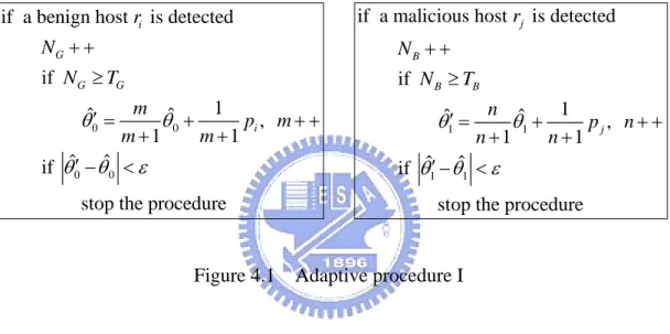
Chapter 4 Adaptive Sequential Hypothesis Testing
When a benign host ri is detected, the value of θ is updated using ˆ0 p , which i is the success rate of FCC attempts sent by the detected benign host . Let
and
i
r
i i
N = +S Fi pi =S Fi i, where and represent, respectively, the numbers of successful and failed FCC attempts sent by when it is detected as benign. Likewise, when a malicious host
i
S Fi
i
r
j
r is detected, the estimate θˆ1 is updated by p , j
which is the success rate of FCC attempts sent by the detected malicious host r . j The formulas can be shown as follows.
0 0 1 1 1 ˆ ˆ 1 1 1 ˆ ˆ 1 1 i j m p m m n p n n θ θ θ θ ′ = + + + ′ = + + +
where m and n represent the numbers of benign and malicious hosts detected and adapted up to now, respectively. The next estimate θˆ0′ is calculated according to the current estimates θˆ0 and the success rate p of FCC attempts when a remote i host is newly determined as benign, and then the value of m is increased by 1. Likewise, the next estimate
i
r
1
ˆ
θ′ can be calculated according to θˆ1 and p once a j new malicious host r is detected, and then n value is increased by 1. j
In the beginning, let m=1 and n= . If 1 m= , the next estimate 0 θˆ0′ will equal to p when the first benign host is discovered. If i n= , the estimate 0 θˆ1′ will also become p when the first malicious host is discovered. Moreover, when j the first few benign hosts are found, almost of FCC attempts sent by them are
Chapter 4 Adaptive Sequential Hypothesis Testing
rate from the first benign host equals to 1, it will make θˆ0′ =1. Similarly, the first few detected malicious hosts have almost zero successful FCC attempts, such that the success rates p are nearly equal to 0. The estimate j θˆ1′ =0 will happen once the
success rates from the first malicious host equals to 0. The situations will cause that the step sizes of moving upward and downward become infinite.
As long as the success rate equals to 1 or it equals to 0, it may let or . The situation will cause that the step sizes of moving upward and download become infinite. 0 ˆ 1 θ′ = 1 ˆ 0 θ′ = 0 0 1 1 0 1 ˆ ˆ 1 1 0 1 0 1 0 1 ˆ ˆ 0 0 0 1 0 1 θ θ θ θ ′ = + + + ′ = + + + = = ⇒
(
)
(
)
1 0 1 0 ˆ 1 ˆ 1 ˆ ˆ F ln upward S ln downward θ θ θ θ ′ − = = ∞ ′ − ′ = = −∞ ′Therefore, the adaptive formulas described above can be used to dynamically adjust the estimates of success rates conditioning on the benign and malicious hypotheses.
Because the earlier detected benign hosts will almost send successful FCC attempts, and the FCC attempts from the earlier detected malicious hosts will almost fail, the adaptive estimates may not be close to the real values if the adaptive procedure is performed in the beginning. So, we choose the duration in which the adaptive procedure is started. Let’s define two parameters and , which denote the thresholds of benign (good) and malicious (bad) hosts. They are used to start the adaptive procedure when the number of the detected benign or malicious host
G
Chapter 4 Adaptive Sequential Hypothesis Testing
is more than or , respectively. At first, only the original TRW algorithm is implemented to examine FCC attempts sent by the remote hosts. As time goes by, it will detect benign and malicious hosts. When , the adaptive procedure will be operated to update the new values of
G T TB G N NB NG ≥TG 0 ˆ
θ′ and m. Likewise, it will be operated to update the values of θˆ1′ and n when . The procedure will be stop if
B
N ≥TB
0 0
ˆ ˆ
θ θ′ − <ε or θ θˆ1′ − ˆ1 <ε . Figure 4.1 shows the adaptive procedure.
0 0
0 0
if a benign host is detected if 1 ˆ ˆ , 1 1 ˆ ˆ if
stop the procedure
i G G G i r N N T m p m m m θ θ θ θ ε + + ≥ ′ = + + + ′ − < + + 1 1 1 1
if a malicious host is detected if 1 ˆ ˆ , 1 1 ˆ ˆ if
stop the procedure
j B B B j r N N T n p n n n θ θ θ θ ε + + ≥ ′ = + + + + ′ − < +
Figure 4.1 Adaptive procedure I
Suppose we can know the number of remote hosts that send connection attempts to local hosts and the ratio of benign to malicious hosts in advance. Therefore we can properly set the thresholds of and to start the adaptive procedure. For example, if there are 1000 remote hosts and the good-to-bad ratio is about 4:1, we can guess that there are approximately 800 benign hosts and 200 malicious hosts. The adaptive procedure will be started after a percentage of benign or malicious hosts are detected.
G
T TB
If and TG =0 TB =0, θˆ0′ and θˆ1′ will be update adaptively since the first
Chapter 4 Adaptive Sequential Hypothesis Testing
the procedure adjusts the two estimates after 25% of benign and malicious hosts are detected, respectively. We can also set the parameters to start the adaptive procedure only from 40% to 60% of hosts which is detected as benign or malicious. It just needs to set that the procedure will be activated when and
. We will show these simulation results in Chapter 5.
320≤NG≤480 80≤NB ≤120
4.2
Scheme 2
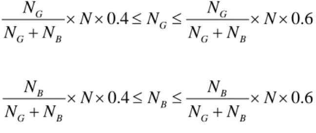
If we only know how many hosts will send connection attempts rather than the good-to-bad ratio, we can calculate the ratio according to the number of hosts detected up to now. Suppose that there are totally N distinct remote hosts, and the TRW algorithm totally discovers benign hosts and malicious hosts so far. We can know that the good-to-bad ratio is
G N NB : G B G B G N N
N +N N +NB , and then we can approximate the expected values of benign and malicious hosts are G
G B N N N +N × and B G B N N N +N × , respectively.
Therefore, we can start the adaptive procedure from 40% to 60% of the expected numbers being detected. That is, the procedure will work when
0.4 0.6 G G G G B G B N N N N N N +N × × ≤ ≤ N +N × × 0.4 0.6 B B B G B G B N N N N N N +N × × ≤ ≤ N +N × ×
Chapter 4 Adaptive Sequential Hypothesis Testing
presented in Chapter 5.
0 0
0 0
if a benign host is detected if 0.4 0.6 1 ˆ ˆ , 1 1 ˆ ˆ if
stop the procedure
i G G G G G B G B i r N N N N N N N N N N m p m m m θ θ θ θ ε + + × × ≤ ≤ × × + + ′ = + + + + + ′ − < 1 1 1 1
if a malicious host is detected if 0.4 0.6 1 ˆ ˆ , 1 1 ˆ ˆ if
stop the procedure
j B B B B G B G B j r N N N N N N N N N N n p n n n θ θ θ θ ε + + × × ≤ ≤ × × + + ′ = + + + + + ′ − <
Figure 4.2 Adaptive procedure II
4.3
Implementation
Based on the hardware implementation introduced in Section 3.3.2, we propose a modified version of implementation. In order to perform SHT, the establishment of FCC requests must be tracked. Generally speaking, if a remote host r sends a connection request to a local host l, and then the host l replies an acknowledgement to the host r, the connection request is regarded as a success. Otherwise, it is a failure. For example, in Figure 4.3, the 1st and 4th connection requests are successful, but the
Chapter 4 Adaptive Sequential Hypothesis Testing
3rd, 6th, and 7th connection requests may be failed.
source IP destination IP No=1 138.230.222.48 140.113.173.14 ← success No=2 140.113.173.14 138.230.222.48 No=3 146.80.28.246 140.113.135.13 ← failure No=4 123.26.187.115 140.113.134.229 ← success No=5 140.113.134.229 123.26.187.115 No=6 128.16.190.43 140.113.159.237 ← failure No=7 162.241.77.123 140.113.96.240 ← failure
Figure 4.3 List of connection
Each connection and the likelihood ratio of each remote host must be recorded. The IP addresses which send or receive connections can be classified as a remote IP of a local IP. A connection is tracked in a connection table indexing by hashing the remote IP address and the local IP address. Each record consists of a 1-bit field marking the connection from local to remote and the other 1-bit field marking the connection from remote to local. The former field set to 1 represents that the local host l has contacted with the remote host r, and the latter field set to 1 represents that the remote host r has contacted with the local host l. The 64-bit IP address is hashed to a 16-bit index, and the memory size of the connection cache is 128K bits. It is shown in Figure 4.4.
Established
Local → Remote Local ← RemoteEstablished
1 bit 1 bit
2 bits 16
2
Connection Cache: 128K bits
(
)
Connection Cache Lookup:
H Local IP, Remote IP →Index
32 bits 32 bits 16 bits
Established
Local → Remote Local ← RemoteEstablished
1 bit 1 bit
Established
Local → Remote Local ← RemoteEstablished
1 bit 1 bit
2 bits 16
2
Connection Cache: 128K bits
(
)
Connection Cache Lookup:
H Local IP, Remote IP →Index
32 bits 32 bits 16 bits
(
)
Connection Cache Lookup:
H Local IP, Remote IP →Index
32 bits 32 bits 16 bits
Chapter 4 Adaptive Sequential Hypothesis Testing
In Figure 4.5, the likelihood ratio of a remote IP address is also recorded in an address table indexing by hashing the remote IP address. Each entry records 16-bit likelihood ratio of the remote IP address. The 32-bit address is also hashed to a 16-bits index, and the memory usage of the address cache is 2M bits.
Address Cache: 2M bits Likelihood ratioΛ
16 bits
(
)
Address Cache Lookup:
H Remote IP Index→
32 bits 16 bits 216 16 bits
Address Cache: 2M bits Likelihood ratioΛ
16 bits
(
)
Address Cache Lookup:
H Remote IP Index→
32 bits 16 bits 216 16 bits
Figure 4.5 Address Table
When a connection is monitored by the scan detection machines, the detection mechanism looks up the connection in the connection table and the corresponding address of remote host in the address table. Then the modified algorithm based on SHT is performed to detect the remote host is benign or malicious. The algorithm is shown in Figure 4.6.
If a remote address r whose likelihood ratio is lower than the upper thresholds and higher than the lower bound sends a FCC request to a local address l, the connection request will be considered as a failure temporarily and the likelihood ratio of remote host r is updated as Λ +F. When a connection is sent by a local host l to a remote host r, if the host r has communicated with the host l, the connection request sent by host r previously must be a success. Therefore, the likelihood ratio of the
Chapter 4 Adaptive Sequential Hypothesis Testing
remote host r will be compensated such that it is updated as Λ − + . F S
Connection ( ) if if set to 1 Connection ( ) if 0 set to 1 if & 0 0 & 1 1 1 local remote F local remote F S malicious conclusion β β α α β α →= ←= →= ← ← − < Λ < − Λ Λ = Λ + ← → Λ → ≥ = = Λ − +
(
)
(
)
if 1 1 adaptive procedure benign conclusion adaptive procedure β α − Λ ≤ −Chapter 5 Simulation Results
Chapter 5
Simulation Results
In this chapter, we will first present simulation results for the performances of the three detection algorithms introduced in Chapter 3, such as SHT, simplified SHT, and RSHT. The desired false positive rate and false negative rate are both assigned to 0.01. As a consequence, we choose α=0.01 and β =0.99 in all simulations. Simulations are performed for 800 benign hosts and 200 malicious hosts.
We will compare the differences between known and unknown of the success rates θ0 and θ1 of connection attempts sent by benign hosts or malicious hosts. In a real network, θ0 and θ1 must be unknown but predictable adaptively. Then, we will also present simulation results for the performance of our proposed adaptive sequential hypothesis testing and compare with the previous algorithms.
5.1
SHT with known
θ
0and
θ
1Chapter 5 Simulation Results
known in advance. In each table shown below, we will orderly demonstrate 4 kinds of data, such as false positive rates (FP), false negative rates (FN), the average numbers of FCC attempts sent by a benign host before being detected (NG), and the
average numbers of FCC attempts sent by a malicious host before being detected (NB).
The horizontal axle represents various values of θ0, and the vertical axle represents various values of θ1.
At first, we show Table 5.1 which represents the step sizes of moving upward and downward for SHT as the values of θ0 and θ1 are changed. It tells that the higher success rate of the benign hypothesis θ0 leads to the larger step size of moving upward, and the lower success rate of the malicious hypothesis θ1 leads to the larger step size of moving downward.
Table 5.2 shows the results of SHT algorithm for the combinations of θ0 and θ1, assuming that they are known in advance. As one can see, the false positive and false negative probabilities are close to the desired values 0.01. The values of NG
and NB, average numbers of FCC attempts sent by a benign and malicious host before
detected, are small, especially when θ0 is larger and θ1 is smaller.
Table 5.3 shows the results of the simplified SHT. The step sizes of moving upward and downward for SHT are changed according the value of θ0 and θ1, but the step sizes for simplified SHT are fixed value. So, we can regard the simplified SHT as a special case of the original SHT. In the tables, we will find the phenomena that the false positive rates increase when θ0 is small, and the false negative rates increase when θ1 is large. For the original SHT, the step size of moving upward must be increasing when θ0 is increasing, and the step size of moving downward must be increasing when θ1 is decreasing. Therefore, when θ0 is smaller and θ1
Chapter 5 Simulation Results
is larger, the step sizes for the simplified SHT are both larger than those for the original SHT. It will exceed the thresholds easily and cause more and more false positives and false negatives.
Because of the step sizes of moving upward and downward, the average numbers of FCC attempts before detected are also different from those of SHT. When there are larger θ0 and smaller θ1, the step sizes of simplified SHT are smaller than those of SHT, so the value of NG and NB are larger. Similarly, the values of observation
are smaller when θ0 is smaller and θ1 is larger.
Table 5.4 is the result of RSHT. Because it only detect the malicious hosts and monitor the benign hosts continuously until they are infected, we can find that the false negative rates are quite low, but it also has much higher false positive rates. Because of the reverse detection, it can detect malicious hosts slightly faster then the SHT algorithm.