國
立
交
通
大
學
統計學研究所
碩
士
論
文
連續型變數之貝氏二階段第二期臨床試驗設計
Bayesian Two-Stage Designs for Phase II Clinical Trials with
Continuous Endpoints
研 究 生:陳思璇
指導教授:蕭金福 教授
連續型變數之貝氏二階段第二期臨床試驗設計
Bayesian Two-Stage Designs for Phase II Clinical Trials with
Continuous Endpoints
研 究 生:陳思璇 Student:Szu-Hsuan Chen
指導教授:蕭金福 Advisor:Chin-Fu Hsiao
國 立 交 通 大 學
統計學研究所
碩 士 論 文
A ThesisSubmitted to Institute of Statistics College of Science
National Chiao Tung University in partial Fulfillment of the Requirements
for the Degree of Master
in Statistics June 2013
Hsinchu, Taiwan, Republic of China
連續型變數之貝氏二階段第二期臨床試驗設計
研究生:陳思璇 指導教授:蕭金福 博士
國立交通大學統計學研究所碩士班
中文摘要
製藥發展是需要長時間和花費的一個過程,而許多機構在執行藥物臨床測試 時,藥物在相對較晚的程序中才宣告失敗停止,因此基於在偵測藥物效能上使用 較快且可靠的方法並且減少受試者人數和試驗所需時間,研發出新式臨床策略或 方法設計,其中的設計是更加有效率不論是在執行上或是花費上在偵測有可能性 的藥物,而新設計在製藥發展中有著迫切的需要。在臨床試驗第二階段(phase II clinical trials),其中兩階段(two-stage)或是多階段(multiple-stage) 無對照組試驗設 計多採用 frequentist 的統計方法,另一方面,相對於 frequentist 另有貝氏(Bayesian) 統計方法,貝氏方法可將相關的先前資訊納入臨床結果分析之中,可使之更加符 合直覺並且對試驗更有幫助。在此篇論文當中,針對連續型變數提出兩種貝氏二 階段藥物效用監控設計,並針對此二設計提出數值範例來示範此二貝氏設計並且 與 frequentist 的統計方法做出比較。Bayesian Two-Stage Designs for Phase II Clinical Trials with Continuous
Endpoints
Student: Szu-Hsuan Chen Advisor: Ph.D. Chin-Fu Hsiao
Institute of Statistics National Chiao Tung University
Abstract
Pharmaceutical development is a lengthy and expensive process and many of these agents fail relatively late in that process. Hence, there is an urgent need of new strategies and methodology for efficient and cost-effective designs to screen potential candidates based on the idea of the proof of the concept for efficacy in a rapid and reliable manner to minimize the total sample size and hence to shorten the duration of the trials. In phase II clinical trials, two-stage or multiple-stage designs with no control group have been proposed based on frequentist statistical approaches. Alternatively, Bayesian methods incorporating relevant prior information into the analysis of the trial results may be more intuitive and helpful. In this thesis, two Bayesian two-stage screening designs based on continuous efficacy endpoints are proposed. Numerical example is presented to illustrate the Bayesian approach. Comparisons with other frequentist approaches are also made.
誌謝
研究所兩年期間,時光飛逝,很快要將學校學生生活告一段落。在學校的兩 年時間裡,非常感謝所上教授給予的教學和指導,和同學鼓勵、砥礪和陪伴相處, 以及所上提供豐富的資源,讓我在研究所時間雖短,但卻獲益良多。 此篇碩士論文的完成,最要感謝我的指導教授蕭金福老師。老師始終細心與 耐心的給予教導和指點,並使用引導和循序漸進的方式,使我學習到了許多研究 的知識、方法和精神。另外,感謝在 group 中的學長學姊時常給予建議和鼓勵, 並和我分享研究的經驗,讓我在研究的路途增添信心,以及感謝賴怡璇博士在百 忙之中給予我論文書寫上的提點。 在學習的路途中,感謝我一群多年陪伴的好友,有了你們的陪伴、鼓勵和支 持,讓我感到很歡樂也很豐富充實,在圖書館念書互相砥礪的時光,讓我非常珍 惜,也助我度過難關和挫折。 最後,感謝我最愛的家人。在我受到挫折或難關之時,總是給予我支持和鼓 勵,並做我最強實的後盾,在我開心時與我分享喜悅,使我感受到加倍的愉悅。 在這段期間受到了無數的幫助,僅將此篇論文獻給我的師長、家人、朋友和 同學,向他們表示我心中無限的感謝。 陳思璇 僅誌于 國立交通大學統計學研究所 中華民國一 0 二年六月Content
中文摘要 .………...
i
Abstract ...………
ii
誌謝 ………...….
iii
Content …………...……….
iv
1. Introduction ………
1
2. Single Threshold Design………..………...
5
3. Dual Threshold Design………….……...………..………...
12
4. Results ………
14
5. Comparison……….
18
6. Conclusion and Discussion ………
21
Appendix………..………
23
References………...………
25
1. Introduction
The development of pharmaceutical products is risky, challenging, slow, costly and time-consuming endeavor. An analysis which takes into account that projects which were neither success nor fair suggests that it usually takes about 10-15 years to develop one new medicine from the time it is discovered to when it is available for commercial marketing and treating patients. The average cost to research and develop each successful drug is estimated to be $800 million to $1 billion and 70% of the cost of pharmaceutical development is wasted on drugs that do not even make it to market. By the time a drug company applies to the Food and Drug Administration (FDA) for marketing approval of a new product, on average it has performed more than 70 clinical studies on at least 4,000 patients. Despite a better understanding of disease etiology and advance in medical technology, there is only 1 out of 10,000 candidates screened in the laboratory that will survive to market launch, and more than 60% of the potential candidates that enter clinical trials fail. Furthermore, the success rate of the phase III stage of the clinical development has fallen by 30% [1]. On the other hand, the development of biomedical science has been raised to cure many diseases nowadays and been full of potential. Nevertheless, the number of the biomedical products and new drugs submitted to the FDA and approved by the FDA does not increase. One of the probable reasons may be that the drug screening process should become more efficient and effective to let the biomedical science fill with full potential. As a result, there is an urgent need of new strategies and methodologies for overall success improving, efficient, and cost-effective designs to screen potential candidates based on the idea of the proof of the concept for efficacy in a rapid and reliable manner to minimize the total sample size and hence to shorten the duration of the trials.
first was developed and tested in the laboratory. Once it is done and ready for testing in the human subjects, a phase Ⅰ trial is conducted. The purpose of the phase Ⅰ trial is to examine the drug tolerance, metabolism and study the drug toxicity in human and also identify the best dose to be used. Then, the phase II trial may employ the best dose identified in the phase Ⅰ study to assess the efficacy of the drug and determine whether it should be tested in further phase Ⅲ trial. The phase Ⅲ trial consists of therapeutic confirmatory studies and establishment of the safety profile by comparing the drug with other compound being used to treat the condition. The phase Ⅳ trial consists of the examination the drug in broad or special population and seeking to identify uncommon adverse events, for example Lawrence et al. [2] and Tan and Machin [3].
To evaluate the biological activity or efficacy of the drug, the phase II trial is conducted. Phase II trials can be a single-stage or a multi-stage design. Among two-stage designs, the approaches commonly used are Gehan design, Simon optimal design, and the minimax design. These designs are based on the frequentist statistical approach. For Simon’s two-stage design, it requires some specific input, including uninteresting level, target level, type Ⅰ error and type II error. The sample sizes are evaluated subjected to the constraint upon the type Ⅰ error and type II error. The idea of the two-stage approach is presented as follows. When the first stage is completed, the trial would be terminated if the response rate does not exceed some critical value indicating that the drug has low efficacy and is not recommended to the next step of the trial. Otherwise, more patients are enrolled and treated in the second stage. After the second stage is completed, the final analysis is performed with the outcomes of the first and the second stage. The drug would be rejected if the overall response rate is less than some critical level and not be recommended to the phase Ⅲ trial. Otherwise, the drug would be recommended to the phase Ⅲ trial. Simon [4] proposed
the “Optimal two-stage designs for phase II clinical trials” with binary response endpoints. Tsou et al. [5] proposed a two-stage screening design based on continuous efficacy endpoints under the framework of Simon two-stage design.
The main concept of Bayesian approach is the incorporation of the prior distribution which brings in the prior experience or information. So, the Bayesian design in Simon [4] allows for the formal incorporation of relevant information from the other resources of the evidence in the monitoring and analysis of the trial. With a Bayesian approach, we can obtain the posterior distribution of the true response rate. This allows us to compute the probability that the response rate falls within the region of interest. For example, we can derive the interval with a 95 per cent probability of containing the true response rate. On the other hand, the frequentist approach cannot answer this kind of questions.
Several Bayesian designs have been proposed for phase II trials, for example methods proposed by Thall [6], Heitjan [7], and Sylverster [8], while most of these are not the real two-stage design but the continuous monitoring design of the trial. In particular, Thall and Simon proposed a design which involves the continual accrual of patients until the new drug is shown with high posterior probability to be either promising or not promising, or until a predetermined maximum sample size is reached. Their design requires the specifications of an informative clinical prior for the response rate of the standard drug which has been found to be the best so far, and a non-informative clinical prior for the response rate of the new drug [6]. In contrast, instead of the prior for the new drug, Heitjan’s design requires the specification of hypothetical skeptical and enthusiastic priors. Both Thall and Simon’s as well as Heitjan’s designs make use of probability distributions for both the response
proportions of the standard drug as well as the new drug. This is unlike the framework of the frequentist designs in which only take account of the response rate of the
standard drug.
Tan and Machin [3] proposed two Bayesian designs for phase II trials which are like the frameworks of designs of Thall [6], Heitjan [7] and Sylverster [8]. The design does not require the specification of a loss or utility function and only need to specify a prior distribution for the response rate of the new drug and not the standard drug as well. It would make the design to be similar to the frequentist approach of two stage phase II clinical trials.
In this thesis, two Bayesian designs for phase II trials with continuous endpoints will be developed. One is the single threshold Bayesian design and another is the dual threshold Bayesian design. These two designs are presented in Section 2 and 3, respectively. The methods to determine the sample size and to determine whether to recommend the drug to the phase Ⅲ trial or not are also proposed. In Section 4, the numerical results of sample sizes and simulation studies are shown. Comparison with Simon design will be given in Section 5. Discussion and conclusion are made in Section 6.
2. Single Threshold Design
We consider a two-stage design for a phase II clinical trial for testing an experimental drug based on continuous response endpoints. In our design, let n1 be the number of patients recruited and treated in the first stage and (possibly) further
2
n be the number of additional patients recruited at stage 2. Let X1i denote the
response of the th
i patient among the n1 patients in stage 1, i1,...,n1and X 2j
denote the responses of the jth patient among the n2 patients in stage 2,
2 1,...,
j n . Total sample size would be N n1 n2 . Because most continuous efficacy endpoints or their log transformation follow normal or approximately normal
distributions, we assume that X and 1i X are normally distributed with a mean of 2j
and a known variance of 2
. Hence, 1 1 1,...., 1 n X X , 1 2 2,...., 2 n
X X are i.i.d. random
variables with common distribution 2
( , )
N . Suppose 2 is known. For convenience of notations, we denote X1 and X2 the sample means of the
responses in the stage 1 and 2, respectively. We also define a pair of variablesY1 X1,
1 2 1 1 1 1 2 2 1 1 2 2 2 1 2 1 2 ... n ... n X X X X n X n X Y n n n n
which are beneficial for following
calculation in two designs. By some algebra (the detail was described in Appendix 1),
we know that X1 is distributed as
2 1 ( , ) N n and X2 is distributed as 2 2 ( , ) N n . Considering the single threshold design (STD), we let U be the target response mean and be the true mean for testing the drug. Then the prior distribution of is assumed as a normal distribution with mean and variance
2
threshold probabilities, at the interim stage and at the end of the trial, respectively. Now, suppose that the (hypothetical) response mean underlying Y1 and Y2 are just larger than the pre-specified U, that is U U, where U is some preselected small value (say between 0 and 0.1 ).
To find the suitable minimum total sample size for this trial design, we enable two constraints to find the smallest sample size. We enable the posterior probability of
over the target response mean U at the end of stage 1, Pr( U|Y1), to be at least1. Moreover, the posterior probability of over the target response mean U at the end of trial, Pr( U |Y Y1, 2), is at least2. We can express two inequalities as
1 1
Pr( U|Y) (1) and
1 2 2
Pr( U |Y Y, ) . (2) According to the Bayesian principal, we obtain that the posterior distribution of
given Y1 is a normal distribution as (the details are given in Appendix 2).
2 2 2 2 1 1 1 2 1 2 2 2 2 2 1 1 1 |Y ~N y n , n (3) n n n
2
1 ~N 1r y r ,r , where 2 1 2 2 1 n r n .By the result of (3), the constraint (1) becomes
2 1 2 2 1 1 1 exp . 2 2 (4) U r y r d r r
Furthermore, by the following computation, we would like to find the posterior distribution of given Y1 and Y2 that enable us to simplify the constraint (2) and find the suitable minimum sample size for the design.
of X1 and X2 given by multiplying a Jacobian factor J . Then we substitute 1 1 X Y, 1 2 1 2 2 1 2 2 n n n X Y Y n n
into expression (5) to get expression (6). The joint distribution of Y1 and Y2 given can be derived as follows,
1 2 ( , | ) f y y 1 2 ( , | ) f x x J , where 1 2 1 1 2 2 2 2 1 0 n n J n n n n n n 1 2 ( | ) ( | ) f x f x J 2 2 1 2 1 2 2 2 2 2 1 2 1 2 ( ) ( ) 1 exp (5) 2 2 2 x x n n n n n n n 2 1 2 1 2 1 2 1 2 2 1 2 2 2 2 2 1 2 1 2 ( ) ( ) 1 exp . (6) 2 2 2 n n n y y y n n n n n n n n n
We then get the joint distribution of Y1, Y2 and by multiplying the joint distribution of Y1 and Y2 given and the prior distribution of that is ( ), that is 1 2 ( , , ) f y y 1 2 ( , | ) ( ) f y y 2 1 2 1 2 1 2 2 1 2 1 2 2 2 2 2 2 2 1 2 1 2 ( ) ( ) 1 1 ( ) exp exp 2 2 2 2 2 n n n y y n n y n n n n n n n
2 1 2 1 2 1 2 2 1 2 1 2 2 2 2 2 2 3 2 2 1 2 1 2 ( ) ( ) 1 ( ) exp . (7) 2 (2 ) 2 2 n n n y y n n y n n n n n n n
By integrating (7) with respect to, we get the joint p.d.f. of Y1 and Y2 as in (8). Expanding three terms of exponential and also separating the terms irrelevant to
out of the integration in expression (8), we get expression (9). 1 2 ( , ) f y y 2 1 2 1 2 1 2 2 1 2 1 2 2 2 2 2 2 3 2 2 1 2 1 2 ( ) ( ) 1 ( ) exp (8) 2 (2 ) 2 2 n n n y y n n y n n d n n n n n
1 2 2 3 2 2 1 2 2 2 2 1 2 1 2 1 2 1 2 1 1 2 2 2 2 2 2 2 2 2 2 1 (2 ) 1 1 1 exp 2 2 2 2 (9) 2 n n c n n n n n n n n n n n y y y d n n
1 2 2 3 2 2 1 2 1 1 1 2 1 1 2 2 2 2 2 2 1 2 2 2 2 1 2 2 2 2 1 (2 ) 1 1 1 exp 2 , (10) 1 2 n n c n n n n n n n y y y n n d n n
where 2 2 2 2 2 2 1 2 1 2 2 1 2 1 2 1 1 2 1 1 2 2 2 2 2 2 2 2 2 2 1 exp 2 2 . 2 2 2 2 n n n n n n n n n n c y y y y y n n n n We multiply and divide a term
2 1 2 2 2 2 1 2 2 2 2 1 exp 1 2 n n y n n simultaneously to
1 2 ( , ) f y y 2 1 2 2 2 2 1 2 2 3 2 2 1 2 2 2 2 1 2 1 2 1 1 1 2 2 2 1 1 2 2 2 2 2 2 1 2 2 2 2 1 2 2 2 2 1 1 exp 1 2 (2 ) 1 1 1 1 exp 2 exp 1 2 n n y n n c n n n n n n n n n n n y y y y n n n n
2 2 1 2 2 2 2 1 2 d n n 2 1 2 2 2 2 1 2 2 3 2 2 1 2 2 2 2 1 2 2 1 2 1 2 2 2 2 2 2 2 2 1 2 2 2 2 1 2 1 2 2 2 2 2 2 2 1 1 exp 1 2 (2 ) 1 1 1 1 exp 2 1 1 2 n n y n n c n n n n n n n n n y y n n n n n n d
2 1 2 2 2 2 1 2 2 3 2 2 1 2 2 2 2 1 2 2 1 2 2 2 2 1 2 2 2 2 1 2 2 2 2 1 1 exp 1 2 (2 ) 1 1 1 exp 1 2 n n y n n c n n n n n n n y n n d n n
2 1 2 2 2 2 1 2 2 3 2 2 1 2 1 2 2 2 2 2 2 2 1 2 1 1 2 exp . (11) 1 1 2 (2 ) n n y n n c n n n n n n n By definition, the conditional p.d.f. of given Y1 and Y2 is to divide the joint p.d.f. of , Y1, and Y2 by the joint pd.d.f. of Y1 and Y2,
1 2 ( | , ) f y y 1 2 1 2 ( , , ) ( , ) f y y f y y
2 1 2 1 2 2 2 2 2 2 2 2 1 2 2 2 2 1 2 1 2 2 2 2 2 2 2 1 2 2 2 2 1 1 1 1 exp 2 1 1 2 2 1 n n n n y y n n n n n n n n 2 1 2 2 2 2 1 2 2 2 2 1 2 1 2 2 2 2 2 2 2 1 1 1 1 exp 1 2 1 2 1 1 n n y n n n n n n 1 2 2 2 2 1 2 1 2 2 2 2 2 2 2 1 1 ~ , . (12) 1 1 n n y N n n n n
We then obtain that the posterior distribution of given Y1 and Y2 is also a normal distribution. By the result of (12), the constraint (2) becomes
2 1 2 2 2 2 1 2 2 2 2 2 1 2 1 2 2 2 2 2 2 2 1 1 1 exp . (13) 1 1 2 2 1 1 U n n y n n d n n n n
Once the sample size has been determined and the trial begins, the n1 patients are recruited in stage 1 of the trial. At the end of stage 1, we evaluated the posterior probability Pr( U |Y1) (Note that Y1now represents the actual data from the stage 1 not the hypothetical data in the design stage). If Pr( U |Y1) is less than
1
, the trial is terminated and that there is insufficient evidence that the drug is efficacious enough to be recommended for the phase Ⅲ trial. On the other hand, if the
posterior probability Pr( U|Y1) is greater than or equal to1, further n2patients would be recruited in stage 2 of the trial. At the end of stage 2, we evaluated the final posterior probability Pr( U |Y Y1, 2). If Pr( U |Y Y1, 2)is less than2, the trial is insufficiently efficacious to be recommended for the phase Ⅲ trial testing. If
1 2
Pr( U|Y Y, )is greater than or equal to2, the product would be tested in the phase Ⅲ trial.
3. Dual Threshold Design
The dual threshold design (DTD) is similar to the single threshold design (STD) except that the sample size of stage 1 is not determined on the posterior probability of
exceeding c, but on the probability that will be less than the ‘no further interest mean response’ L. This represents the average response mean below which the investigators would have no further interest in the new drug. The value L acts as the lower threshold of average response mean, as opposed to the upper threshold represented by U . The first constraint of stage 1 becomes
1 1
Pr( L|Y) (14) and the constraint of stage 2 is the same as the one in the STD, as in (2),
1 2 2
Pr( U |Y Y, ). (15) Now, suppose that the (hypothetical) response mean underlying Y1 is just smaller than the pre-specified L, that is LL and the (hypothetical) response mean underlying Y2 is just larger than the pre-specified U, that is U U, where
L
and U are some preselected small values.
By the same computation in the STD, constraints (14) and (15) become
2 2 1 1 2 2 2 2 0 1 1 1 1 exp , where 2 2 (16) L r y r n d r r r n
and 2 1 1 2 2 2 2 2 1 2 2 2 2 2 1 2 2 2 2 1 2 2 2 2 1 1 1 1 1 1 1 exp , (17) 1 1 2 2 1 1 1 1 1 1 U n y n y n n d n n n n
according to these two constraints.
Once the sample sizes have been determined and the trial stared, the n1 patients are recruited in stage 1 of the trial. At the end of stage 1, we evaluated the posterior probability Pr( L|Y1) (Note that Y1now represents the actual data from the stage 1 not the hypothetical data in the design stage). If Pr( L|Y1) is greater than or equal to 1, the trial is terminated and that there is insufficient evidence that the drug is efficacious enough to be recommended for the phase Ⅲ trial. On the other hand, if the posterior probability Pr( L|Y1) is less than 1, further n2patients would be recruited in stage 2 of the trial. At the end of stage 2, we evaluated the final posterior probability Pr( U |Y Y1, 2). If Pr( U |Y Y1, 2)is less than2, the trial is insufficiently efficacious to be recommended for the phase Ⅲ trial testing. If
1 2
Pr( U|Y Y, )is greater than or equal to2, the product would be tested in the phase Ⅲ trial.
4. Result
4.1 Sample size of Single Threshold Design
The purpose of the phase Ⅱ trial is to assess the efficacy of the new drug. Before the trial, we know relatively little information regarding the efficacy of the new drug being test. It makes sense to make a prior distribution in the design stage. Especially, we make the use of the normal distribution which centers on the upper thresholdU . We also note that the use of normal distribution allow us easily update the prior distribution from the normal data.
Before the start of the trial, we help the investigators provide some parameters of the normal prior distribution and also the value of U. For suggestion, if the variance of the data is large, we recommend the choice of the larger variance parameter of the prior distribution. Also, the mean of the prior distribution is recommended to be around the target average response rate.
In this section, we give some examples to illustrate our designs. Tables 1-24 demonstrate the Single Threshold Design for several combinations of parameters with
1.0 U , U 0.5, 6, 8, 13, 2 1 , 2 2 , 2 4 , 2 9 . The values of are from 8 to 12 centered around U . The rational selections of
1, 2
are
0.6, 0.7 ,
0.6, 0.8 and
0.7, 0.8 as listed in the tables. The
tabulated results contain the minimum required sample sizes determined by using a program of numerical technique written in C corresponding to combinations of
U
, , and .
For example, as shown in the first row and the first column of the Table 1
displaying the result corresponding to ( , 1 2)(0.6, 0.7), U 9, 8, 2 1, 112 patients should be enrolled in the stage 1. When the stage 1 trial is completed, if
1
recruit additional 62 patients (which is173 112 ) in stage 2.
We investigate some properties of the Single Threshold Design. If the difference between center (mean) of the prior distribution and target average response rate
U
increases, both the sample sizes of two stages (stage 1 and stage 2) increase. On the other hand, with regard to the same prior distribution, as U increases, the target becomes harder to reach, thus the sample size N and n1 increase. Also, from Table 1 and Table 9, if the sample variance increases, the both the sample sizes, n1 and
1
Nn , increase.
It also can be seen that larger values of2result in larger sample sizes N. Similarly, larger values of 1 result in larger sample sizes n1. The values of 1 and
2
are desired success probabilities that the average response rates will exceed the target response value, U, in the interim and the final stage, respectively. Hence, the larger the values of 1 and 2, the greater the amount evidence from data needed.
We now investigate the connection between the sample size and the value of
U
. For the selected values of parameters other than U , sample size N decrease as
U
increase. It make intuitive sense since having data with larger advantage over U means that the threshold probability can be attained with a smaller sample size. For example, the elements in the first row and first column of the Table 1 and Table 2 respectively, the sample size 69 in Table 2 with larger U 1.0 is smaller than the sample size 173 in Table 1 with smaller U 0.5.
4.2 Sample size of Dual Threshold Design
In this section, we give some examples to illustrate the Dual Threshold Design. The same vague normal distribution used in the Single Threshold Design is used in the Dual Threshold Design. Also, the suggestions for the prior distribution selection
are the same as those given in the Single Threshold Design. Tables 25-29 illustrate the Dual Threshold Design for several combinations of parameters with U 0.5,
0.5
L
, 6, 8, 2 42,2 52, 2 62, 2 72, 2 152. The value of
is from 8 to 12 centered around U . The rational selection of
1, 2
are
0.6, 0.7 ,
0.6, 0.8 and
0.7, 0.8 as listed in the tables. The tabulated results
contain the suitable minimum sample size determined by using a program of numerical technique written in C corresponding to combinations of U, L, , and .
For example, the element in the first row and the first column of the Table 25
displays the result corresponding to ( , 1 2)(0.6, 0.7), U 9, 8, 2 42. The entry is 49(38). That means at least 38 patients required for stage 1 trial. When the stage 1 trial is completed, if Pr( L|Y1) is greater or equal to 1, the trial is terminated for futility. Otherwise, we recruit another 11 (which is49 38 ) patients in stage 2.
We investigate some properties of the Dual Threshold Design. If the mean of the prior distribution increases and the other parameters are fixed, the sample size, n1, of stage 1 increases but the total sample size N decreases. On the other hand, with regard to the same prior distribution, as Uincreases, the target becomes harder to reach. Thus, the sample size N increases but the stage 1 sample size n1stays the same.
It also can be seen that larger values of2result in larger sample sizes N. Similarly, larger values of 1 result in larger sample sizes n1. Both Single Threshold Design and Dual Threshold Design have the same trend.
of L. For the selected values of parameters other than L, the total sample size N
increases as L increases. To avoid the too large sample size, the values L and U are restricted to 0.5 in the Dual Threshold Design.
5. Comparison with Tsou et al. [5]
5.1 Threshold probabilities
The optimal and minimax designs proposed by Tsou et al. [5] are two commonly used methods in phase Ⅱ two-stage trials with continuous endpoints. We are interest in evaluating the threshold probabilities 1 and 2 corresponding to these designs and making a comparison with the single threshold design and the dual threshold design.
We choose to work with sample size recommended by Tsou et al. [5] and its decision criteria corresponding to the type Ⅰ and Ⅱ error probabilities of (0.10,0.10), (0.05,0.20) and (0.05,0.10), respectively. We evaluate the value of the probability Pr( U |Y Y1, 2)given the average response rates Y1 and Y2 to be overall critical level C2 recommended by Tsou et al. [5], where if the observed overall sample mean is less than C2 , the trial would be terminated.
1 2
Pr( U|Y Y, ) will give us the desired threshold probability 2. The choice of the prior distribution of is N(U, 2 )2 for each combination of parameters in the single threshold design because the sample size of N(U, 2 )2 in STD is smaller and much similar to the sample size of Tsou et al. [5]. Also, the choice of the prior
distribution of in the dual threshold design is N(U, 6 )2 for the same reason. For the single threshold design, 1 is evaluated by Pr( U|Y1) given the average response rate Y1 to be the critical value of stage 1 C1 recommended by Tsou et al. [5], where if the observed sample mean is less than C2, the trial would be terminated. For the dual threshold design, 1 is evaluated by Pr( L|Y1) also given the average response rate Y1 to be the critical value of stage 1 C1
recommended by Tsou et al. [5].
and the dual threshold design, respectively. The values of 2 are quite low because the overall critical level C2 is lower than the target average response rate U although it is higher than L. Thus the drugs recommended to the phase Ⅲ trial have quite low posterior probabilities of exceeding the target average response rate
U
. It also can be seen that the values of 1 is quite low for both STD and DTD. It may give us some sense that low 1 in the Tsou et al. [5] lower down the chance of early termination of the trial.
5.2 Probabilities of early termination and expected sample sizes
We further compare our designs with the designs of Tsou et al. [5] by evaluating the probability of early termination (PET) and the expected sample size (EN) of the single threshold and the dual threshold design. For the single threshold design, the
PET is given byPrPr
U |Y1
1. We take Y1 as a random variable with the normal distribution 2 1 ( , ) N n . For the dual threshold design, the PET is given by
1
1PrPr L|Y , where Y1 also follows the normal distribution
2 1 ( , ) N n .
As for the expected sample size, EN is given by n1
1 PET n
2.Table 34-35 and 36-37give the values of PET and EN corresponding to STD and DTD, respectively, with L U 0.5 and ( , 1 2)(0.6, 0.7), (0.6, 0.8) and (0.7, 0.8). The values of PET in STD are in the range 0.20 to 0.35 and suggest not stopping at the end of the stage 1. The values of PET in STD are lower than what they are for the design of Tsou et al. [5]. For the design of Tsou et al. [5], the PET is in the range 0.45 to 0.75. For the DTD, the values of PET are in the range 0.75 to 0.85 and suggest that the design is likely to recommend terminate at the end of stage 1.
For EN, the range is from 40 to 378 for the STD and from 28 to 98 for the DTD. Both generally higher than what they are in Tsou et al. [5]. There is intuitive sense that the value of 1 and PET is related because the lower value of 1 keeps the lower sample size. So, the STD and the DTD keep the higher sample sizes than sample size of Tsou et al. [5].
6. Conclusion and Discussion
In this thesis, our objective is proposing new Bayesian designs for the phase Ⅱ clinical trial based on continuous efficacy endpoints. Although Bayesian methods are not in general use for its unfamiliarity and difficulty of implementation to investigators, we believe that Bayesian methods can bring much more information to analysis of the phase Ⅱ trial.
To free from complexity of implementation of Bayesian approach, we focus on developing designs which are relatively simple and easy compared to original Bayesian approaches. For example, we do not require specific utility or loss function before the trial. We maintain the adoption of Bayesian designs to process two Bayesian designs for phase II clinical trials. These designs were developed to be familiar to two-stage frequentist phase II clinical trials. The Bayesian approach allows the conjunction of relevant prior information and then the result in that manner is more conservative, informative and accurate.
We found that the choice of the variance 2of the prior distribution has strong impact on the sample size of the trial. If the variance 2 is too small, it would cause a large sample size (larger than general sample size of the phase Ⅱ trial). So, we would suggest investigators choose the variance parameter which is not too small. The choices of the values of threshold probabilities 1 and 2 have strong impact on the sample size. As shown in Table 1 ─ 29, the higher threshold probabilities, the larger sample sizes. Although we can lower down the threshold probability to pursue smaller sample size for low cost of the trial, we might lower down the probability of detecting the true effect. There is a trade-off between pursuing a smaller sample size and the threshold probabilities not too low for sure the accuracy of the clinical trial.
than the sample size of Tsou et al. [5]. However, in the Table 30-33, we know our designs have high threshold probabilities. It shows that our designs is stricter and have higher probability of detecting the true effect. It is a intuitive sense that more information and more accuracy worth higher sample size to ensure the drug efficacy in the clinical trial.
Bayesian method is a good approach alternative to the frquentist approach for phase Ⅱ clinical trials. Bayesian methods incorporating relevant prior information into the analysis of the trial results may be more intuitive and helpful. In this thesis, two new Bayesian designs with continuous endpoints in phase Ⅱ trials have been developed and made to be easy used and friendly to the investigators. Our next step may extend our two designs to take the time-to-event variables into consideration.
Appendix
Lemma 1 Let 1 1 1,...., 1 n X X be i.i.d. 2 ( , )N random variable. Define Y1 the sample mean of
1 1 1,...., 1 n X X . Then, Y1 is distributed as 2 1 ( , ) N n . Proof:
According to the property of the normal distribution, the addition of independent and identically distributed (i.i.d.) normal distributed random variable preserves the normal distribution. Hence, we derive the mean and variance of Y1 and Y2 to identify the exact distribution.
1
1 1 1 1 1 1 1 1 1 1 1 1 1 1 1 ... 1 1 ... ... n n n X X E Y E E X X E X E X n n n
1 1 1 1 1 ... n n n and
1
1 1 1 1 1 1 1 1 2 1 1 2 1 1 1 1 1 ... 1 1 ... ... n n n X XVar Y Var Var X X Var X Var X
n n n
2 2 2 2 1 2 2 1 1 1 1 1 ... n . n n n So, Y1is distributed as 2 1 ( , ) N n . Lemma 2Since that Y |follows distribution as
2 1 ( , ) N n and is distributed asN( , 2). The posterior distribution of given Y , | Yis
2
1 , ,
2 1 2 2 1 n r n . Proof:
Let g Y
|
and h
denote the p.d.f. of2 1 ( , ) N n and N( , 2), respectively. Then, the posterior p.d.f. of given Y is denoted as k
|Y
which has the following property,
|
|
k Y g Y h
2 2 2 2 1 1 1 1 exp 2 2 2 2 y n n .If we eliminate all constant factors (including factors involving only y ), we have
2 2 2 2 2 1 1 2 2 1 2 | exp 2 y n n k Y n .This can be simplified by completing the square to read
2 2 1 | exp 2 r y r k Y r , where 2 1 2 2 1 n r n .That is, the posterior p.d.f. of the parameter is obviously normal distribution with
mean 2 2 2 2 1 1 2 2 2 2 2 2 1 1 1 y n n y n n n and variance 2 2 1 2 2 1 n n [10].
References
1. Mercky prospects; pharmaceuticals. The Economist. 2002;364:60.
2. Lawrence M. Friedman, Curt D. Furberg and David L. DeMets. Fundamentals of Clinical Trials, Fourth edition. Springer; 2010.
3. Say-Beng Tan and David Machin (2002). Bayesian two-stage designs for phase II clinical trials. Statistics In Medicine, 21, 1991-2012.
4. Simon, R. (1989). Optimal two-stage designs for phase II clinical trials,
Controlled Clinical Trials, 10, 1-10.
5. Tsou, H. H., Hsiao, C. F., Chow, S. C., and Liu, J. P. (2008). A two-stage design for drug screening trials based on continuous endpoints, Drug Information
Journal, 42, 253-262.
6. Thall PF, Simon R (1994). Practical Bayesian guidelines for phase IIB clinical trials. Biometrics, 50(2), 337–349.
7. Heitjan DF (1997). Bayesian interim analysis of phase II cancer clinical trials.
Statistics in Medicine, 16(16), 1791–1802.
8. Sylvester RJ (1988). A Bayesian approach to the design of phase II clinical trials.
Biometrics, 44(3), 823–836.
9. Kevin P. Murphy (2007). Conjugate Bayesian analysis of the Gaussian distribution.
10. Robert V. Hogg, Joseph W. Mckean and Allen T. Craig. Introduction to Mathematical Statistics, Sixth edition. Prentice Hall; 2004.
Tables
Table 1. Minimum required sample size for single threshold design (U 0.5, 6).
prior U N(n1) N(8,1) N(9,1) N(10,1) N(11,1) N(12,1) 9 173 (112) 64 (24) * * * 302 (112) 142 (24) * * * 302 (173) 142 (64) * * * 10 289 (204) 173 (112) 64 (24) * * 489 (204) 302 (112) 142 (24) * * 489 (289) 302 (173) 142 (64) * * 11 410 (302) 289 (204) 173 (112) 64 (24) * 729 (428) 489 (204) 302 (112) 142 (24) * 729 (410) 489 (289) 302 (173) 142 (64) * * : no solution
For each value of U , the first, the second and third rows correspond to ( , 1 2) of (0.6, 0.7), (0.6, 0.8) and (0.7, 0.8), respectively.
Table 2. Minimum required sample size for single threshold design (U 1.0, 6).
prior U N(n1) N(8,1) N(9,1) N(10,1) N(11,1) N(12,1) 9 69 (51) 25 (11) * * * 95 (51) 46 (11) * * * 95 (69) 46 (25) * * * 10 112 (90) 69 (51) 25 (11) * * 144 (90) 95 (51) 46 (11) * * 144 (112) 95 (69) 46 (25) * * 11 156 (130) 112 (90) 69 (51) 25 (11) * 193 (130) 144 (90) 95 (51) 46 (11) * 193 (156) 144 (112) 95 (69) 46 (25) * * : no solution
For each value of U , the first, the second and third rows correspond to ( , 1 2) of (0.6, 0.7), (0.6, 0.8) and (0.7, 0.8), respectively.
Table 3. Minimum required sample size for single threshold design (U 0.5, 6). prior U N(n1) N(8,2) N(9,2) N(10,2) N(11,2) N(12,2) 9 109 (64) 54(19) * * * 198(64) 123(19) * * * 198(109) 123(54) * * * 10 163(108) 109(64) 54(19) * * 278(108) 198(64) 123(19) * * 278(163) 198(109) 123(19) * * 11 219(152) 163(108) 109(64) 54(19) * 364(152) 278(108) 198(64) 123(19) * 364(219) 278(163) 198(109) 123(54) * * : no solution
For each value of U , the first, the second and third rows correspond to ( , 1 2) of (0.6, 0.7), (0.6, 0.8) and (0.7, 0.8), respectively.
Table 4. Minimum required sample size for single threshold design (U 1.0, 6).
prior U N(n1) N(8,2) N(9,2) N(10,2) N(11,2) N(12,2) 9 43(29) 20(8) * * * 64(29) 38(8) * * * 64(43) 38(20) * * * 10 65(49) 43(29) 20(8) * * 89(49) 64(29) 38(8) * * 89(65) 64(43) 38(20) * * 11 87(69) 65(49) 43(29) 20(8) * 113(69) 89(49) 64(29) 38(8) * 113(87) 89(65) 64(43) 38(20) * * : no solution
For each value of U , the first, the second and third rows correspond to ( , 1 2) of (0.6, 0.7), (0.6, 0.8) and (0.7, 0.8), respectively.
Table 5. Minimum required sample size for single threshold design (U 0.5, 6). prior U N(n1) N(8,4) N(9,4) N(10,4) N(11,4) N(12,4) 9 77 (40) 48 (15) * * * 151 (40) 114 (15) * * * 151 (77) 114 (48) 75 (8) * * 10 104 (62) 77 (40) 48 (15) * * 188 (62) 151 (40) 114 (15) * * 188 (104) 151 (77) 114 (48) 75 (8) * 11 131 (84) 104 (62) 77 (40) 48 (15) * 227 (84) 188 (62) 151 (40) 114 (15) * 227 (131) 188 (104) 151 (77) 114 (48) 75 (8) * : no solution
For each value of U , the first, the second and third rows correspond to ( , 1 2) of (0.6, 0.7), (0.6, 0.8) and (0.7, 0.8), respectively.
Table 6. Minimum required sample size for single threshold design (U 1.0, 6).
prior U N(n1) N(8,4) N(9,4) N(10,4) N(11,4) N(12,4) 9 29 (17) 16 (6) * * * 47 (17) 33 (6) * * * 47 (29) 33 (16) * * * 10 41 (28) 29 (17) 16 (6) * * 60 (28) 47 (17) 33 (6) * * 60 (41) 47 (29) 33 (16) * * 11 52 (38) 41 (28) 29 (17) 16 (6) * 73 (38) 60 (28) 47 (17) 33 (6) * 73 (52) 60 (41) 47 (29) 33 (16) * * : no solution
For each value of U , the first, the second and third rows correspond to ( , 1 2) of (0.6, 0.7), (0.6, 0.8) and (0.7, 0.8), respectively.
Table 7. Minimum required sample size for single threshold design (U 0.5, 6). prior U N(n1) N(8,9) N(9,9) N(10,9) N(11,9) N(12,9) 9 58(25) 44(13) * * * 125(25) 108(13) * * * 125(58) 108(44) 91(28) * * 10 71(35) 58(25) 44(13) * * 141(35) 125(25) 108(13) * * 141(71) 125(58) 108(44) 91(28) * 11 83(46) 71(35) 58(25) 44(13) * 158(46) 141(35) 125(25) 108(13) * 158(83) 141(71) 125(58) 108(44) 91(28) * : no solution
For each value of U , the first, the second and third rows correspond to ( , 1 2) of (0.6, 0.7), (0.6, 0.8) and (0.7, 0.8), respectively.
Table 8. Minimum required sample size for single threshold design (U 1.0, 6).
prior U N(n1) N(8,9) N(9,9) N(10,9) N(11,9) N(12,9) 9 20(10) * * * * 36(10) * * * * 36(20) 30(13) 22(6) * * 10 25(15) 20(10) * * * 43(15) 36(10) * * * 43(25) 36(20) 30(13) 22(6) * 11 31(20) 25(15) 20(10) * * 49(20) 43(15) 36(10) * * 49(31) 43(25) 36(20) 30(13) 22(6) * : no solution
For each value of U , the first, the second and third rows correspond to ( , 1 2) of (0.6, 0.7), (0.6, 0.8) and (0.7, 0.8), respectively.
Table 9. Minimum required sample size for single threshold design (U 0.5, 8). prior U N(n1) N(8,1) N(9,1) N(10,1) N(11,1) N(12,1) 9 307 (199) 113 (42) * * * 537 (199) 253 (42) * * * 537 (307) 253 (113) * * * 10 513 (363) 307 (199) 113 (42) * * 869 (363) 537 (199) 253 (42) * * 869 (513) 537 (307) 253 (113) * * 11 728 (537) 513 (363) 307 (199) 113 (42) * 1296 (537) 869 (363) 537 (199) 253 (42) * 1296 (728) 869 (513) 537 (307) 253 (113) * * : no solution
For each value of U , the first, the second and third rows correspond to ( , 1 2) of (0.6, 0.7), (0.6, 0.8) and (0.7, 0.8), respectively.
Table 10. Minimum required sample size for single threshold design (U 1.0,
8 ). prior U N(n1) N(8,1) N(9,1) N(10,1) N(11,1) N(12,1) 9 122 (90) 44 (19) * * * 169 (90) 82 (19) * * * 169 (122) 82 (44) * * * 10 199 (160) 122 (90) 44 (19) * * 255 (160) 169 (90) 82 (19) * * 255 (199) 169 (122) 82 (44) * * 11 276 (231) 199 (160) 122 (90) 44 (19) * 342 (213) 255 (160) 169 (90) 82 (19) * 342 (276) 255 (199) 169 (122) 82 (44) * * : no solution
For each value of U , the first, the second and third rows correspond to ( , 1 2) of (0.6, 0.7), (0.6, 0.8) and (0.7, 0.8), respectively.
Table 11. Minimum required sample size for single threshold design (U 0.5, 8 ). prior U N(n1) N(8,2) N(9,2) N(10,2) N(11,2) N(12,2) 9 193(114) 95(33) * * * 352(114) 219(33) * * * 352(193) 219(95) * * * 10 289(191) 193(114) 95(33) * * 494(191) 352(114) 219(33) * * 494(289) 352(193) 219(95) * * 11 389(271) 289(191) 193(114) 95(33) * 647(271) 494(191) 352(114) 219(33) * 647(389) 494(289) 352(193) 219(95) * * : no solution
For each value of U , the first, the second and third rows correspond to ( , 1 2) of (0.6, 0.7), (0.6, 0.8) and (0.7, 0.8), respectively.
Table 12. Minimum required sample size for single threshold design (U 1.0,
8 ). prior U N(n1) N(8,2) N(9,2) N(10,2) N(11,2) N(12,2) 9 76(51) 35(14) * * * 114(51) 67(14) * * * 114(76) 67(35) * * * 10 115(87) 76(51) 35(14) * * 158(87) 114(51) 67(14) * * 158(116) 114(76) 67(35) * * 11 154(122) 115(87) 76(51) 35(14) * 201(122) 158(87) 114(51) 67(14) * 201(154) 158(116) 114(76) 67(35) * * : no solution
For each value of U , the first, the second and third rows correspond to ( , 1 2) of (0.6, 0.7), (0.6, 0.8) and (0.7, 0.8), respectively.
Table 13. Minimum required sample size for single threshold design (U 0.5, 8 ). prior U N(n1) N(8,4) N(9,4) N(10,4) N(11,4) N(12,4) 9 136 (70) 84 (27) * * * 268 (70) 202 (27) * * * 268 (136) 202 (84) 133 (14) * * 10 185 (110) 136 (70) 84 (27) * * 334 (110) 268 (70) 202 (27) * * 334 (185) 268 (136) 202 (84) 133 (14) * 11 233 (149) 185 (110) 136 (70) 84 (27) * 402 (149) 334 (110) 268 (70) 202 (27) * 402 (233) 334 (185) 268 (136) 202 (84) 133 (14) * : no solution
For each value of U , the first, the second and third rows correspond to ( , 1 2) of (0.6, 0.7), (0.6, 0.8) and (0.7, 0.8), respectively.
Table 14. Minimum required sample size for single threshold design (U 1.0,
8 ). prior U N(n1) N(8,4) N(9,4) N(10,4) N(11,4) N(12,4) 9 51 (30) 28 (11) * * * 84 (30) 58 (11) * * * 84 (51) 58 (28) * * * 10 72 (49) 51 (30) 28 (11) * * 107 (49) 84 (30) 58 (11) * * 107 (72) 84 (51) 58 (28) * * 11 92 (67) 72 (49) 51 (30) 28 (11) * 130 (67) 107 (49) 84 (30) 58 (11) * 130 (92) 107 (72) 84 (51) 58 (28) * * : no solution
For each value of U , the first, the second and third rows correspond to ( , 1 2) of (0.6, 0.7), (0.6, 0.8) and (0.7, 0.8), respectively.
Table 15. Minimum required sample size for single threshold design (U 0.5, 8 ). prior U N(n1) N(8,9) N(9,9) N(10,9) N(11,9) N(12,9) 9 102(43) 77(22) * * * 222(43) 192(22) * * * 222(102) 192(77) 161(49) * * 10 126(63) 102(43) 77(22) * * 251(63) 222(43) 192(22) * * 251(126) 222(102) 192(77) 161(49) * 11 148(81) 126(63) 102(43) 77(22) * 280(81) 251(63) 222(43) 192(22) * 280(148) 251(126) 222(102) 192(77) 161(49) * : no solution
For each value of U , the first, the second and third rows correspond to ( , 1 2) of (0.6, 0.7), (0.6, 0.8) and (0.7, 0.8), respectively.
Table 16. Minimum required sample size for single threshold design (U 1.0,
8 ). prior U N(n1) N(8,9) N(9,9) N(10,9) N(11,9) N(12,9) 9 35(18) 24(8) * * * 64(18) 52(8) * * * 64(35) 52(24) 39(10) * * 10 45(26) 35(18) 24(8) * * 76(26) 64(18) 52(8) * * 76(45) 64(35) 52(24) 39(10) * 11 55(35) 45(26) 35(18) 24(8) * 87(35) 76(26) 64(18) 52(8) * 87(55) 76(45) 64(35) 52(24) 39(10) * : no solution
For each value of U , the first, the second and third rows correspond to ( , 1 2) of (0.6, 0.7), (0.6, 0.8) and (0.7, 0.8), respectively.
Table 17. Minimum required sample size for single threshold design (U 0.5, 13 ). prior U N(n1) N(8,1) N(9,1) N(10,1) N(11,1) N(12,1) 9 810(524) 297(111) * * * 1417(524) 666(111) * * * 1417(810) 666(297) * * * 10 1354(958) 810(524) 297(111) * * 2294(958) 1417(524) 666(111) * * 2294(1354) 1417(810) 666(297) * * 11 1923(1417) 1354(958) 810(524) 297(111) * 3421(1416) 2294(958) 1417(524) 666(111) * 3421(1923) 2294(1354) 1417(810) 666(297) * * : no solution
For each value of U , the first, the second and third rows correspond to ( , 1 2) of (0.6, 0.7), (0.6, 0.8) and (0.7, 0.8), respectively.
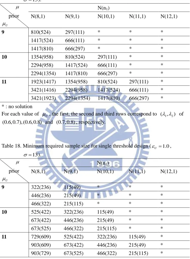
Table 18. Minimum required sample size for single threshold design (U 1.0,
13 ). prior U N(n1) N(8,1) N(9,1) N(10,1) N(11,1) N(12,1) 9 322(236) 115(49) * * * 446(236) 215(49) * * * 466(322) 215(115) * * * 10 525(422) 322(236) 115(49) * * 673(422) 446(236) 215(49) * * 673(525) 466(322) 215(115) * * 11 729(609) 525(422) 322(236) 115(49) * 903(609) 673(422) 446(236) 215(49) * 903(729) 673(525) 466(322) 215(115) * * : no solution
For each value of U , the first, the second and third rows correspond to ( , 1 2) of (0.6, 0.7), (0.6, 0.8) and (0.7, 0.8), respectively.
Table 19. Minimum required sample size for single threshold design (U 0.5, 13 ). prior U N(n1) N(8,2) N(9,2) N(10,2) N(11,2) N(12,2) 9 508(299) 250(87) * * * 928(299) 577(87) * * * 928(508) 577(250) * * * 10 764(504) 508(299) 250(87) * * 1303(504) 928(299) 577(87) * * 1303(764) 928(508) 577(250) * * 11 1027(714) 764(504) 508(299) 250(87) * 1707(714) 1303(504) 928(299) 577(87) * 1707(1027) 1303(764) 928(508) 577(250) * * : no solution
For each value of U , the first, the second and third rows correspond to ( , 1 2) of (0.6, 0.7), (0.6, 0.8) and (0.7, 0.8), respectively.
Table 20. Minimum required sample size for single threshold design (U 1.0,
13 ). prior U N(n1) N(8,2) N(9,2) N(10,2) N(11,2) N(12,2) 9 200(134) 91(37) * * * 300(134) 177(37) * * * 300(200) 177(91) * * * 10 304(228) 200(134) 91(37) * * 416(228) 300(134) 177(37) * * 416(304) 300(200) 177(91) * * 11 406(321) 304(228) 200(134) 91(37) * 530(321) 416(228) 300(134) 177(37) * 530(406) 416(304) 300(200) 177(91) * * : no solution
For each value of U , the first, the second and third rows correspond to ( , 1 2) of (0.6, 0.7), (0.6, 0.8) and (0.7, 0.8), respectively.