駕駛員閃避突發障礙物及不同駕駛風格之腦波反應研究

全文

(1)國立交通大學電機與控制工程學系碩士論文. 駕駛員閃避突發障礙物及不同駕駛風格之腦波反應研究 A Study of EEG Correlates Unexpected Obstacle Dodging Task and Driving Style. 研究生：董行偉指導教授：林進燈教授中華民國九十四年七月.

(2) 駕駛員閃避突發障礙物及不同駕駛風格之腦波反應研究 A Study of EEG Correlates of Unexpected Obstacle Dodging Task and Driving Style 研究生：董行偉指導教授：林進燈. 教授. Student： Hsing-Wei Tung Advisor：Prof. Chin-Teng Lin. 國立交通大學電機與控制工程學系碩士論文 A Thesis Submitted to Institute of Electrical and Control Engineering College of Electrical Engineering and Computer Science National Chiao Tung University in partial Fulfillment of the Requirements for the Degree of Master in Electrical and Control Engineering June 2005 Hsinchu, Taiwan, Republic of China. 中華民國九十四年七月.

(3) 博碩士論文授權書本授權書所授權之論文為本人在＿國立交通＿大學(學院)＿電機與控制工程＿系所＿＿＿C＿＿＿＿組＿＿九十三＿＿學年度第＿二＿學期取得＿碩＿士學位之論文。論文名稱：＿駕駛員閃避突發障礙物及不同駕駛風格之腦波反應研究指導教授：＿林進燈＿教授＿＿＿＿＿＿＿＿＿＿＿＿＿＿＿＿＿＿＿＿＿＿＿ 1.5同意不同意本人具有著作財產權之上列論文全文(含摘要)資料，授予行政院國家科學委員會科學技術資料中心(或改制後之機構)，得不限地域、時間與次數以微縮、光碟或數位化等各種方式重製後散布發行或上載網路。本論文為本人向經濟部智慧財產局申請專利(未申請者本條款請不予理會)的附件之一，申請文號為:______________，註明文號者請將全文資料延後半年再公開。 2.5同意不同意本人具有著作財產權之上列論文全文(含摘要)資料，授予教育部指定送繳之圖書館及國立交通大學圖書館，基於推動讀者間「資源共享、互惠合作」之理念，與回饋社會及學術研究之目的，教育部指定送繳之圖書館及國立交通大學圖書館得以紙本收錄、重製與利用；於著作權法合理使用範圍內，不限地域與時間，讀者得進行閱覽或列印。本論文為本人向經濟部智慧財產局申請專利(未申請者本條款請不予理會)的附件之一，申請文號為:______________，註明文號者請將全文資料延後半年再公開。 3.5同意不同意本人具有著作財產權之上列論文全文(含摘要)，授予國立交通大學與台灣聯合大學系統圖書館，基於推動讀者間「資源共享、互惠合作」之理念，與回饋社會及學術研究之目的，國立交通大學圖書館及台灣聯合大學系統圖書館得不限地域、時間與次數，以微縮、光碟或其他各種數位化方式將上列論文重製，並得將數位化之上列論文及論文電子檔以上載網路方式，於著作權法合理使用範圍內，讀者得進行線上檢索、閱覽、下載或列印。論文全文上載網路公開之範圍及時間 – 本校及台灣聯合大學系統區域網路：年月日公開校外網際網路：年月日公開上述授權內容均無須訂立讓與及授權契約書。依本授權之發行權為非專屬性發行權利。依本授權所為之收錄、重製、發行及學術研發利用均為無償。上述同意與不同意之欄位若未鉤選，本人同意視同授權。研究生簽名：學號： 9212605 （親筆正楷）（務必填寫）日期：民國 1.. 九十四. 年. 七. 月. 二十七. 日. 本授權書請以黑筆撰寫並影印裝訂於書名頁之次頁。.

(4) 國家圖書館博碩士論文電子檔案上網授權書本授權書所授權之論文為本人在＿國立交通＿大學(學院)＿電機與控制工程＿系所＿＿＿C＿＿＿組＿九十三＿＿學年度第＿二＿學期取得＿碩＿士學位之論文。論文名稱：＿駕駛員閃避突發障礙物及不同駕駛風格之腦波反應研究＿＿指導教授：＿林進燈＿教授＿＿＿＿＿＿＿＿＿＿＿＿＿＿＿＿＿＿＿＿. 5同意. 不同意. 本人具有著作財產權之上列論文全文(含摘要)，以非專屬、無償授權國家圖書館，不限地域、時間與次數，以微縮、光碟或其他各種數位化方式將上列論文重製，並得將數位化之上列論文及論文電子檔以上載網路方式，提供讀者基於個人非營利性質之線上檢索、閱覽、下載或列印。上述授權內容均無須訂立讓與及授權契約書。依本授權之發行權為非專屬性發行權利。依本授權所為之收錄、重製、發行及學術研發利用均為無償。上述同意與不同意之欄位若未鉤選，本人同意視同授權。研究生簽名：（親筆正楷）日期：民國. 學號： 9212605 （務必填寫）九十四. 年. 七. 月. 二十七. 日. 1. 本授權書請以黑筆撰寫，並列印二份，其中一份影印裝訂於附錄三之一(博碩士論文授權書)之次頁﹔另一份於辦理離校時繳交給系所助理，由圖書館彙總寄交國家圖書館。.

(5) 駕駛員閃避突發障礙物及不同駕駛風格之腦波反應研究研究生：董行偉. 指導老師：林進燈教授. 國立交通大學電機與控制工程學系碩士班. 摘要. 本論文探討當駕駛員夜間開車，閃避前方突如其來的障礙物時，受到不預期刺激的腦波反應。我們使用虛擬實境結合腦波量測分析來研究夜間駕車之腦波特性，此為本論文之一大創新；實驗場景為夜間直線高速公路之駕車環境，並有不預期之障礙物突然出現在駕駛員前方車道，使其產生一不預期差異之認知狀態，紀錄並觀察腦波訊號，此外另設計有警示標誌出現來提醒駕駛員將出現障礙物，進而來觀察有警示與無警示下兩者之腦波差異。我們探討兩個主題，首先是觀察駕駛員看到障礙物時的認知狀態。透過獨立成分分析將原始腦波分離為數個獨立之成分，進而使用交叉相關性分析比較各個駕駛員之間獨立成分之關聯性，實驗結果發現與心理負荷相關之腦波獨立成分來源在顱頂中央(CPz)，且於 6~7Hz 頻帶有功率增強之情形。其次，我們藉由駕駛員閃避障礙物之行為模式，從其駕駛車輛之行進軌跡以及方向盤轉向之資訊，辨別出不同之駕駛風格，分為過度駕駛與適當駕駛以分析不同駕駛風格之腦波特性，經由獨立成分分析後，找到可用於駕駛風格鑑別之腦波特徵，其在顱頂(Cz)位置之 10Hz,20Hz 頻帶中具有能量上的差異，可藉此來估測駕駛員之駕駛特性。. i.

(6) A Study of EEG Correlates of Unexpected Obstacle Dodging Task and Driving Style. Student： Hsing-Wei Tung. Advisor： Prof. Chin-Teng Lin. Institute of Electrical and Control Engineering National Chiao-Tung University. ABSTRACT In this thesis, we want to study the EEG relates of surprising status and driving style. Accidents usually caused by lack of alertness and awareness have a high fatality rate especially in night driving environments. It becomes extremely dangerous in some situations such as the appearance of an unexpected obstacle in the middle of the road. Combining the technology of virtual reality (VR), a realistic driving environment is developed to provide stimuli to subjects in our research. The VR scene designed in our experiment is driving a car on the freeway at nighttime. Independent Component Analysis (ICA) is used to decompose the sources in the EEG data. ICA combined with power spectrum analysis and correlation analysis is employed to investigate the EEG activity related to surprising level and driving style. According to our experimental results, the appearance of ERP at CPz is highly correlated to the surprising status. Furthermore, the level of surprising status can be evaluated with the amplitude of the ERP. An extension analysis of driving style has also been further studied in the experiments. It is observed that the magnitudes of ERP power spectrum at 10Hz and 20Hz are different respecting to different driving styles.. ii.

(7) 誌謝感謝父母親董須平、吳明麗自幼的栽培，感謝林進燈老師以及學長姐們梁勝富、趙文鴻、陳玉潔、吳瑞成、黃騰毅、黃冠智的指導，也感謝同學高士政、陳俞傑、李欣弘及學弟們蕭力碩、謝弘義、謝宗哲的幫忙，還有謝謝大家的支持。. iii.

(8) Contents Abstract in Chinese .....................................................................................................................1 Abstract in English......................................................................................................................ii 誌謝 .........................................................................................................................................iii Contents .....................................................................................................................................iv List of Figures ............................................................................................................................vi List of Tables.............................................................................................................................vii. Chapter 1. Introduction..........................................................................................................1. Chapter 2 Experimental Design and Setup .........................................................................5 2.1. Virtual Reality(VR)-Bsed Environmental Setup .........................................................6. 2.2. EEG Signals Acquisition .............................................................................................8. 2.2.1. Subjects............................................................................................................8. 2.2.2. EEG Signals Acquisition .................................................................................8. 2.3. Experimental design ..................................................................................................10. Chapter 3. EEG Data Analysis.............................................................................................15. 3.1. Independent Components Analysis (ICA).................................................................15. 3.2. Power Spectrum Analysis..........................................................................................19. 3.3. Correlation Analysis ..................................................................................................20. 3.4. The Procedures of EEG Data Analysis......................................................................20. 3.4.1. Data Processing of Unexpected Obstacle Dodging.......................................21. 3.4.2. Data Processing of Driving Style Analysis....................................................24. Chapter 4 4.1. Experimental Results.........................................................................................28. EEG Correlates of Surprising Status .........................................................................28. 4.1.1. Results of ICA Decomposition Analysis .......................................................29. 4.1.2. Within-Subject Analysis ................................................................................30. 4.1.3. Cross-Subjects Analysis ................................................................................33 iv.

(9) 4.2. EEG Correlates of Driving Styles .............................................................................34. 4.2.1. The Category of Driving Styles.....................................................................35. 4.2.2. Results of ICA decomposition Analysis ........................................................35. Chapter 5 5.1. Discussions..........................................................................................................39. The Relationship between EEG Changes and Surprising Status...............................39. 5.1.1. Surprising Status Influence Region on Human Cortex .................................40. 5.1.2. Surprising Level Correlates Without-Cue Condition ....................................42. 5.1.3. Reaction Time Variations in Subject’s Surprising Level ...............................43. 5.1.4. The Power Increasing of 2Hz and 6Hz at Centro-Parietal Midline...............44. 5.2. Driving Style Classification by EEG Signal Analysis...............................................45. Chapter 6. Conclusions and Future Work..........................................................................47. References. v.

(10) List of Figures Fig. 2-1. Block diagram of the virtual-reality (VR)-based driving simulation environment and physiological signal acquisition..........................................................................................5 Fig. 2-2. Flowchart of the VR-based highway scene development environment. The dynamic models and shapes of the 3D objects in the VR scene are created and linked to the WTK library to form a complete interactive VR simulated scene. ..............................................6 Fig. 2-3. The range of steering angle..........................................................................................7 Fig. 2-4. The scalp map of 10-20 International System of Electrode Placement. ......................9 Fig. 2-5. The experimental scene..............................................................................................10 Fig. 2-6. Experimental setting. ................................................................................................. 11 Fig. 2-7. The VR scene in the With-Cue task. ..........................................................................12 Fig. 2-8. Ground plane representation of the ” with-cue” task.................................................12 Fig. 2-9. Ground plane representation of the ” without-cue” task............................................13 Fig. 2-10. Driving Trajectory Types .........................................................................................14 Fig. 3-1. The scalp topographies of ICA weighting matrix W..................................................18 Fig. 3-2. ERP Extraction from EEG Raw Data. .......................................................................21 Fig. 3-3. Signal processing flowchart of surprise status analysis.............................................22 Fig. 3-4. Independent component analysis and artifact-component rejection..........................23 Fig. 3-5. Surprise-Related Components Selection....................................................................24 Fig. 3-8. Evaluation procedure of averaged power spectrum for subject i of component j (Process II)........................................................................................................................27 Fig. 3-9. The evaluated averaged power spectrum. ..................................................................27 Fig. 4-1. ICA components of subjects 6 and 10. Red circle: Eye blinking; Yellow circle: Channel noise; Green circle: Muscle movements; Blue circle: Eyes movements. ..........29 Fig. 4-2. The seven subjects have a common ICA component located at around CPz correlated to the without-cue tasks. ...................................................................................................30 vi.

(11) Fig. 4-3. Results of the common ICA component on CPz channel. .........................................31 Fig. 4-4. The ERP images of subject 5 in without- and with-cue tasks at CPz channel...........31 Fig. 4-5. The EEG power spectrum of subject 5 at CPz channel corresponding to without-cue tasks and with-cue tasks. ..................................................................................................32 Fig. 4-6. The relationship between reaction time and amplitude in without-cue task..............33 Fig. 4-7. The peaking time changes between without- and with-cue tasks on source channel.34 Fig. 4-8. The amplitude changes between without- and with-cue tasks on source channel. ....34 Fig. 4-9. Different driving styles in unexpected obstacle dodging task : (a) Over-driving, (b) Under-driving. ..................................................................................................................35 Fig. 4-10. The weighting matrix of ICA analysis for driving style classification. ...................36 Fig. 4-11. The component average power comparison.............................................................37 Fig. 5-4. Power spectrum of the ICA component 4 ..................................................................46. List of Tables Table 1 : The Relationship between Surprising status and Reaction time................................44 Table 2 : The Power increase of Specific Band ........................................................................45. vii.

(12) Chapter 1 Introduction. Throughout the world in countries where is a substantial volume of vehicular traffic, the incidence of road collisions, and the resulting deaths, injuries and property damage, is regarded as a significant social problem. In many instances, the traffic accidents often occur from late at night to early morning, and especially when the driver is distracted. Driving at night is one of the most hazardous situations commonly faced by the driver. It is now well established that the rate of fatal traffic accidents is 3 to 4 times higher at night than at daytime . It is established that under nighttime conditions many visual abilities such as spatial resolution, contrast discrimination, stereoscopic depth perception, accommodation, response and reaction time are degraded [1]. So that nighttime driving is a serious issue for more investigations, especially for the appearance of unexpected obstacles. This critical issue motivates us to discover what reactions happened in the human brain when a driver encountered the unexpected obstacle. Driver reactions to the sudden incidental appearance of an object such as a child rushing out may differ depending on the driver’s attention to the peripheral scene. A more complete understanding of the attentive mechanisms of the brain will improve driver responses and increase driving safety. For mental workload studies, when assessing workload in driving, as well as task demand, is an important loading factor. For example, the workload of freeway driving when operating a high-speed car should be assessed in terms of information processing load and time on nighttime driving. It must be noted that the consequences of task performance over a period, such as fatigue increment and vigilance decrement, has a complex relationship with the effects of task demand, when the demand is mainly mental. There are many studies in 1960s and 1970s dealing with the effects of time-on-task on 1.

(13) vigilance or sustained attention [2]. Some of these studies manipulated task demand such as event rate and described the change in performance over time-on-task [3]. In recent mental workload studies, on the other hand, the effects of time-on-task have been neglected. Jex defined mental workload as “the operator’s evaluation of the attentional load margin”[4]. Eggemeier defined it as “the degree of process capacity that is expanded during task performance”[5]; and Wickens wrote that “the concept of workload is fundamentally defined by this relationship between resource supply and task demand”[6]. There are several measures and assessment techniques that are said to be sensitive to mental workload. Among them are heart rate variability (HRV), event-related potentials (ERP), dual-task methods, and the two major rating scales known as the SWAT (the Subjective Workload Assessment Technique) and the NASA-TLX(Task Load Index). We take ERPs as an important measure for our investigation. K.Eba et al. introduced a real driving experiment to observe the brain activities related to driving situation [7]. In a car driving task with and without an unexpected dummy doll rushing out, they recorded the homodynamic activities of the frontal lobe by near infrared spectroscopy (NIRS). As a result, they concluded that the right rostromedial prefrontal cortex plays an important role in spatial attentive recognition of driving scene. By the improvement of driving simulation technology, we can use the driving simulation to save the time and costs. The use of driving simulation for vehicle design and driver perception studies is expanding rapidly. This is largely because how applicable driving simulation is to the real world is unclear, however analyses of perceptual criteria carried out in driving simulation experiments are controversial. Keneny and Panerai [8] suggested that, in driving simulators with a large field of view, longitudinal speed can be estimated correctly from visual information. On the other hand, recent psychophysical studies have revealed an unexpectedly important contribution of vestibular cues in distance perception and steering, prompting a re-evaluation of the role of visuo–vestibular interaction in driving simulation studies. For the event related subjects, some specific features of EEG are expected to occur in the brain activities respecting to different situations. Moreover, the Event-Related Potential [9-11] 2.

(14) analysis has widely used for the EEG data processing. The interested target is called a single event within the experiments, thus the brain activities related to the event were extracted for further analysis. The key problem to perform such a work is the inability to dynamically quantify cognitive changes in the human capacity. A way to determine the relationship between different stimuli and human cognitive responses accompanying correct, incorrect and absent motor responses is the use of event-related brain potential (ERP) signals. Moreover, we concern about the unexpected obstacle dodging task related to the ERP response. There are some similar studies about incongruent cognitive state. In these studies, they proposed an incongruent situation to induce negative brain activities by visual or auditory stimulus [11]. The broad negative wave peaks in the surface EEG around 400 ms after a semantically incongruous word in a meaningful sentence [12, 13]. And there are also many studies proposed that the waveform can be elicited in response to semantic processing of non-verbal stories [14]. In our study, we want to investigate the EEG dynamics related to the unexpected obstacle dodging task. With combining the technology of virtual reality (VR), a realistic stimuli environment is provided to subjects in our research. A surprising task is provided to the subjects with a broken-down car appears in the middle of the road. The subjects are requested to dodge the broken-off car as soon as possible and dodge collision in the experiments. One of the main purpose of our research is to investigate EEG changes relate to surprising status by anglicizing the subjects’ EEG features corresponding to the With-Cue task and the Without-Cue task. Another is the classification of different driving style in unexpected obstacle dodging tasks. This thesis is organized as follow. In Chapter 2, the experimental design is introduced in first section, and the following section is about the experimental setup of hardware and software. In section three, the subjects and data acquisition are introduced here. In Chapter 3, we explore the analysis procedure by applying ICA, power spectrum analysis, and correlation coefficient. The experimental results of EEG signals are described in Chapter 4. Detailed. 3.

(15) discussions of our experimental results are given in Chapter 5. Finally, the conclusions are summarized in Chapter 6.. 4.

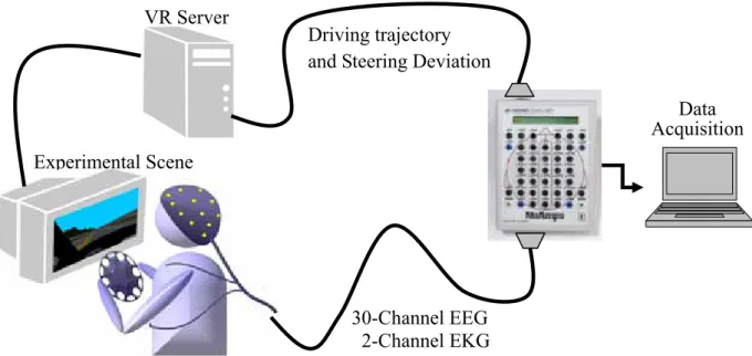
(16) Chapter 2 Experimental Design and Setup. The main purpose of our research is to investigate the EEG features correlated surprising status. As we have mentioned in Chapter 1, the previous studies of incongruent context were focused on semantics [11-18]. With combining the technology of virtual reality (VR), a realistic stimuli environment is provided to subjects in our research. The experimental setup is shown in Fig. 2-1. In our experiments, subjects are asked to sit in front of a monitor with their hands on the steering wheel to control the car in the VR scene. A 30-channel EEG electrode cap was mounted on the subject’s head and a 2-channel electrodes was put at the middle of the chest to record the physiological EEG, EOG and EKG signals. The physiological signals and the event data from the scene are then send through the Neuroscan biomedical signal amplifier to the data acquisition laptop.. VR Server. Driving trajectory and Steering Deviation Data Acquisition. Experimental Scene. 30-Channel EEG 2-Channel EKG. Fig. 2-1. Block diagram of the virtual-reality (VR)-based driving simulation environment and physiological signal acquisition. 5.

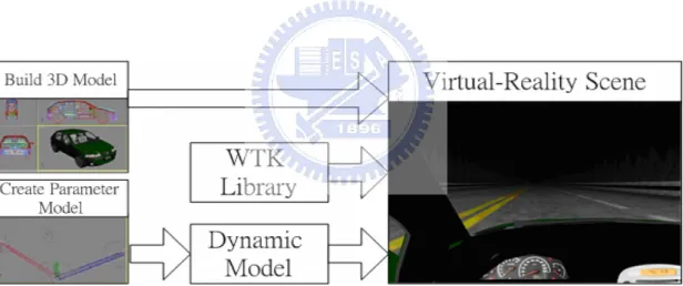
(17) 2.1 Virtual Reality(VR)-Based Environmental Setup. In this study, the VR scene was generated by the Virtual- Reality technology with a WTK library as showing in Fig. 2-2. Firstly, the 3DS-max is used to build three-dimensional models accurately for a true system (such as the road) and to define the parameters of each model (such as the width of the road). Then, the C program including the WTK library is used and its library function is called up to move the three-dimensional models. The 3DS-man software is popular graphic software to create a three-dimensional model. The WTK library is an advanced cross-platform development environment for high-performance, real-time and three-dimensional graphics applications.. Fig. 2-2. Flowchart of the VR-based highway scene development environment. The dynamic models and shapes of the 3D objects in the VR scene are created and linked to the WTK library to form a complete interactive VR simulated scene.. The VR scene was displayed on a color XVGA 42” Plasma Display Panel (PDP) to simulate a night driving scene on freeway. The subjects are asked to sit in front of the PDP with the distance 60cm between subject and displayer. The freeway VR scene we used in this research includes four lanes from left to right of the road. The distance from the left side to the right side of the road is equally divided into 256 6.

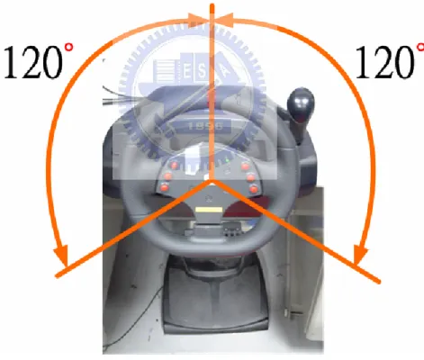
(18) points (digitized into values 0-255), where the width of each lane and the car are 60 units and 32 units, respectively. The frame rate of the scene changes as the driver is driving at a fixed velocity of 120 km/hr on freeway. The subjects are asked to keep the car in the VR scene in the middle of the third lane (left-counting). Furthermore, the angle of the steering wheel is considered as an important issue in this research, which indicates the dynamic response of subjects. The steering angle is recorded at the same time. The angle range of the steering wheel we used in the experiments is -120 ﾟ~120 ﾟ, as shown in Fig. 2-3.. Fig. 2-3. The range of steering angle.. 7.

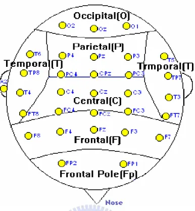
(19) 2.2 EEG Signals Acquisition. 2.2.1 Subjects Ten healthy volunteers (including seven males and three females) with no history of gastrointestinal, cardiovascular, or vestibular disorders participated in the experiment of the motion-sickness study. They were requested not to smoke, drink caffeine, use drugs, or drink alcohol, all of which could influence the central and autonomic nervous system for a week prior to the main experiment. Screening confirmed that subjects were free of past or current psychiatric and neurological disorders. Three subjects’ EEG data were excluded for further analysis because of the unexpected artifacts (ex: severe head shaking) within the data. A total of seven subjects (one female and six males, ages from 21 to 26, all right-handed) with normal or corrected normal vision participated in the VR-based unexpected-incident driving experiment where EEG signals were simultaneously recorded.. 2.2.2 EEG Signals Acquisition. An electrode cap is mounted on the subject’s head for signal acquisition on the scalp. A standard for the placement of EEG electrodes was proposed by Jasper in 1958, which is known as the 10-20 International System of Electrode Placemen was used in one experimental cap. An illustration of the 10-20 system is shown in Fig. 2-4.. 8.

(20) Fig. 2-4. The scalp map of 10-20 International System of Electrode Placement.. All channels were referenced to the reference channel (behind the right ear) with the input impedance 5 kΩ. The EEG data were recorded with 16-bit quantization level at a sampling rate (SR) of 500 Hz. The data is recorded by the Scan NuAmps Express system (Compumedics Ltd., VIC, Australia). A 500-pt high pass filter with a cut-off frequency at 1 Hz is used to remove breathing artifacts. The width of the transition band of the high pass filter is 0.2 Hz. A 30-pt low pass filter is then applied to the signal with the cut-off frequency at 50 Hz to remove muscle artifacts and line noise. The transition band width of the low pass filter is 7 Hz. The Independent Component Analysis (ICA) [19-26, 27-28] is also applied to the EEG signal to remove the artifacts including eye movement or blinking more detailed will be discussed in Section 3.4... 9.

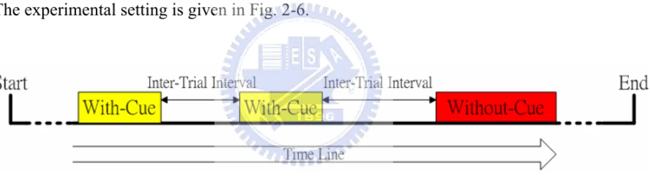
(21) 2.3 Experimental design. Fig. 2-5. The experimental scene.. The fatality rate of nighttime driving accidents is much higher than that in daytime because the driver’s abilities of vision, vehicle control are obviously declined in nighttime. The response time of the drivers will also be slow due to the range of visibility is diminished in nighttime. It becomes extremely dangerous in some situations, such as the appearance of an unexpected obstacle in the middle of the road. The VR scene in our experiment is design on the freeway in nighttime, as shown in Fig. 2-5. The subject is asked to control the simulated car in the VR scene with the steering wheel and keep the car in the middle of the third lane. A surprising task is provided to the subjects with a broken-down car appears in the middle of the road. The subjects are requested 10.

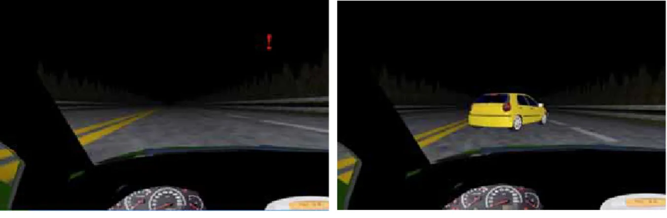
(22) to dodge the broken-off car as soon as possible and dodge collision in the experiments. Two different tasks are designed for the further EEG investigation; they are the Without-Cue task and With-Cue task. In the Without-Cue task, the unexpected broken-off cars will appear randomly in front of the simulated car appeared without any cue. By contrast, an exclamation mark will appear before the broken-off car in the With-Cue task, to reduce the surprising level to subjects. One of the main purpose of our research is to investigate EEG changes relate to surprising status by anglicizing the subjects’ EEG features corresponding to the With-Cue task and the Without-Cue task. As long as the status of surprising which is a natural response without any expecting effect will be investigated in this study,. Thus, the Inter-trial intervals (ITIs) are set from 10 to 30 seconds, and differ from trial to trial randomly to dodge the anticipating effect of subjects. The experimental setting is given in Fig. 2-6.. Fig. 2-6. Experimental setting.. Each subject participated in three nighttime driving experiments in three different days. The experiments start from a 1~5 minutes training session and follows by two 30-min sessions including a 5 min break between these two experiments . The EEG signals as well as the steering angle trajectory are recorded synchronously during the experiments.. The exclamation mark is designed to provide a simple hint to subjects before the broken-off car appears in the With-Cure task. The position of the exclamation mark is shown in Fig. 2-7(a).. 11.

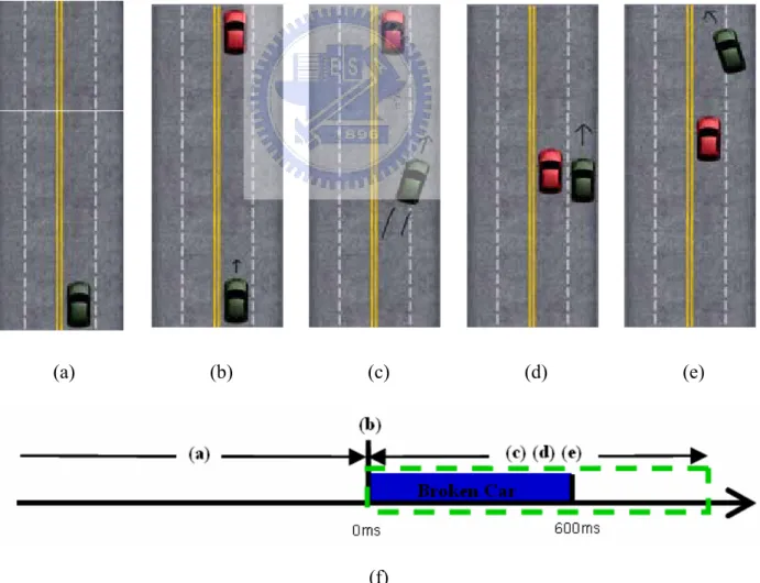
(23) (a). (b). Fig. 2-7. The VR scene in the With-Cue task.. ! (a). (b). (c). (f) Fig. 2-8. Ground plane representation of the ” with-cue” task.. 12. (d). (e).

(24) The durations of the cue and the unexpected obstacle appearance are 1 sec and 600ms, respectively. The sketch map of the With-Cue task is given in Fig. 2-8. The green cars in the figure are the simulated car which control led by the subjects, and the red cars are the broken-off car park on the road. The subjects are asked to control the car with the steering wheel to dodge the broken-off car and to keep the car in the middle of the third lane. In Fig. 2-8(a), the cue appears on the VR scene to provide a hint. After the appearance of the cue, a broken-off car appears in the middle of the road it lasting and last for 600 ms as shown in Fig. 2-8(b). The subjects are asked to dodge the broken-off car and to drive the car back to the third lane after dodging, as shown in Figs. 2-8(c), (d) and (e). The schema of the time arrangement is shown in Fig. 2-8(f).. (a). (b). (c). (f) Fig. 2-9. Ground plane representation of the ” without-cue” task.. 13. (d). (e).

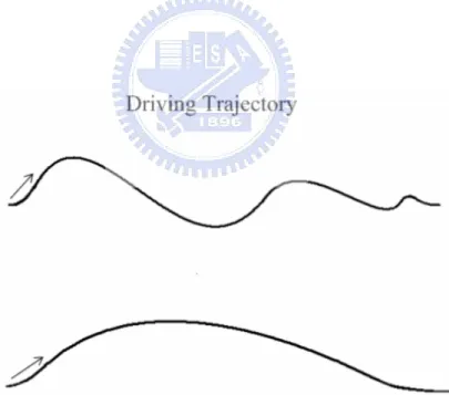
(25) By contrast, there is no hint for the obstacle in the Without-cue task. The subjects have to response to the situation immediately when they see the broken-off car. The design of the experiment protocol is given in Fig. 2-9. The surprise-related ERPs are expected to occur in the Without-Cue task. Thus the EEG signal within the green broken line in Fig. 2-9 is the interested target which is extracted for further analysis procedure.. In a view of different personalities of drivers, let us then consider the different driving styles of drivers. In our experiments, the driving trajectory and steering angle are also recorded. According to these driving indices, we can take this advantage to identify the driver’s driving trajectory. And the driving style of one driver, moreover, can be classified into two standard styles as following figure.. Fig. 2-10. Driving Trajectory Types. 14.

(26) Chapter 3 EEG Data Analysis. Two analysis procedures are proposed in this thesis to investigate the EEG relates of surprising status and driving style. The analysis methods which used in the procedure are firstly introduced in this chapter, followed by the proposed analysis produces. Independent Component Analysis (ICA) is used to decompose the sources in the EEG data. ICA combined with power spectrum analysis and correlation analysis is employed to investigate EEG activity related to surprising level and driving style.. 3.1 Independent Components Analysis (ICA). The joint problems of EEG source segregation, identification, and localization are very difficult since the EEG data collected from any point on the human scalp includes activity generated within a large brain area, and thus, problem of determining brain electrical sources from potential patterns recorded on the scalp surface is mathematically underdetermined [26]. Although the resistivities between the skull and brain are different, the spatial smearing of EEG data by volume conduction does not involve significant time delay and suggests that the ICA algorithm is suitable for performing blind source separation on EEG data by source identification from that of source localization. We attempt to completely separate the twin problems of source identification and source localization by using a generally applicable ICA. 15.

(27) Thus, the artifacts including the eye-movement (EOG), eye-blinking, heart-beating (EKG), muscle-movement (EMG), and line noises can be successfully separated from EEG activities. The ICA is a statistical “latent variables” model with generative form:. x( t ) = A s( t ) ,. (1). where A is a linear transform called a mixing matrix and the S i are statistically mutually independent. The ICA model describes how the observed data are generated by a process of mixing the components S i . The independent components S i (often abbreviated as ICs) are latent variables, meaning that they cannot be directly observed. Also the mixing matrix A are assumed to be unknown. All we observed are the random variables xi , and we must estimate both the mixing matrix and the ICs S i using the xi . Therefore, given time series of the observed data x(t ) = [ x1 (t ) x 2 (t ) ⋅ ⋅ ⋅ x N (t )]T in. N-dimension, the ICA is to find a linear mapping W such that the unmixed signals u(t) are statically independent.. u( t ) = W x( t ) ,. (2). Supposed the probability density function of the observations x can be expressed as: p( x ) = det( W ) p( u ). ,. (3). the learning algorithm can be derived using the maximum likelihood formulation with the log-likelihood function derived as: N. L( u ,W ) = log det( W ) + ∑ log pi ( ui ) , i =1. (4). Thus, an effective learning algorithm using natural gradient to maximize the log-likelihood with respect to W gives:. ∆W ∝. [. ]. ∂ L( u ,W ) T W W = I − ϕ ( u )uT W , ∂W 16. (5).

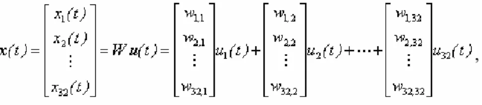
(28) where the nonlinearity T. ∂ p( u N ) ⎡ ∂ p( u1 ) ⎤ ∂u N = ⎢− ∂ u1 ϕ( u ) = − " − ⎥ p( u ) ⎢⎣ p( u1 ) p( u N ) ⎥⎦ , ∂ p( u ) ∂u. (6). T and W W in Eq. (5) rescales the gradient, simplifies the learning rule and speeds the. convergence considerably. It is difficult to know a priori the parametric density function p(u ) ,. which plays an essential role in the learning process. If we choose to approximate the estimated probability density function with an Edgeworth expansion or Gram-Charlier expansion for generalizing the learning rule to sources with either sub- or super-gaussian distributions, the nonlinearity ϕ (u ) can be derived as: ⎧u − tanh( u ) : for super - gaussian sources, ⎩u + tanh( u ) : for sub - gaussian sources,. ϕ( u ) = ⎨. (7). Then,. [ ⎩[I + tanh( u )u. ] ]W : sub - gaussian. ⎧ I − tanh( u )uT − uuT W : super - gaussian. ∆W = ⎨. T. − uu. T. (8). Since there is no general definition for sub- and super-gaussian sources, we choose p( u ) =. 1 2. (N (1, 1) + N (-1, 1) ). and. p( u ) = N (0,1) sec h 2(u) for sub- and super-gaussian,. respectively, where N ( µ , σ 2 ) is a normal distribution. The learning rules differ in the sign before the tanh function and can be determined using a switching criterion as: ⎧κ = 1 : super - gaussian ∆W ∝ [I − K tanh( u )uT − uuT ]W , where ⎨ i ⎩κ i = −1 : sub - gaussian. (9). where. κ i = sign(E {sec h 2 ( ui )}E {ui2 }− E{tanh( ui )ui }). (10). is repeats the elements of N-dimensional diagonal matrix K. After ICA training, we can obtain 30 ICA components u(t) decomposed from the measured 30-channel EEG data x(t). 17.

(29) , (11) Fig. 3-1 shows the scalp topographies of ICA weighting matrix W corresponding to each ICA component by spreading each wi,j into the plane of the scalp, which provides spatial information about the contribution of each ICA component (brain source) to the EEG channels, e.g., eye activity was projected mainly to frontal sites, and the drowsiness-related potential is on the parietal lobe to occipital lobe, etc. We can observe that the most artifacts and channel noises included in EEG recordings are effectively separated into ICA components 1 and 3 in Fig. 3-1.. Eye-blinkin. Eye-movement. Fig. 3-1. The scalp topographies of ICA weighting matrix W.. 18.

(30) 3.2 Power Spectrum Analysis. Analysis of changes in spectral power and phase can characterize the perturbations in the oscillatory dynamics of ongoing EEG. Applying such measures to the activity time courses of separated independent component sources avoids the confounds caused by misallocation of positive and negative potentials from different sources to the recording electrodes, and by misallocation to the recording electrodes activity that originates in various and commonly distant cortical sources. The spectral analysis for each ICA component decomposed from 30 channels of the EEG signals. The FFT processes for each ICA component data decomposed from 30 channels of the EEG signals and the processes are described as following. The sampling rate of EEG is 250Hz. The power spectrum density (PSD) of each ERP is evaluated with the spectral analysis process. The activity power spectrum of the ERP is calculat by averaging the PSDs. The ICA data power spectrum time series for each session consisted of ICA data power estimates at 50 frequencies (from 1 to 50 Hz). The same procedure of power spectrum analysis was applied to 30 EEG channels for comparisons. The input EEG signal is x[n] . And we can consider computing X [k ] by separating x[n] into two (N/2)-point sequences consisting of the even-numbered points in x[n] and the. odd-numbered points in x[n] . n. WN2 = e −2 j ( 2π / N ) = e − j 2π ( N / 2 ) = WN / 2. (12). The PSDs was calculated as following equations: X [k ] =. ( N / 2 ) −1. ∑ x[2r ]WNrk/ 2 +WNk r =0. = G[k ] + WNk H [k ],. 19. ( N / 2 ) −1. ∑ x[2r + 1]W r =0. rk N /2. k = 0,1,..., N − 1,. (13).

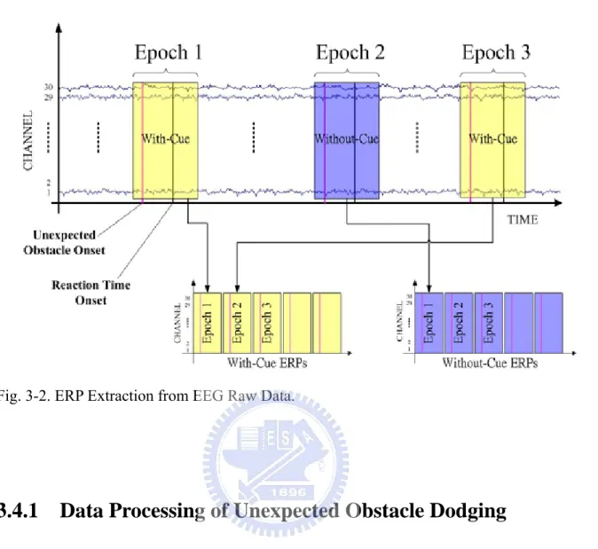
(31) 3.3 Correlation Analysis. In order to find the EEG dynamic between different subjects’ ICA components and EEG channel distribution, we computed the correlation coefficient between the time course of EEG channel signals and the concurrent changes in the ICA spectrum of EEG signals by using the Pearson Correlation Coefficient: Corrxy =. ∑ (x − x ) * ( y − y ) ∑ (x − x ) * ∑ ( y − y ) 2. 2. ,. (14). where Corrxy is defined as a statistical measure of the linear relationship between two random variables x and y, x and y is the expected value of x and y, respectively.. 3.4 The Procedures of EEG Data Analysis. The main purpose of this research is to investigate the subject’s EEG response related to the unexpected obstacle dodging tasks. The unexpected obstacle is also called a single event within the experiments. Thus, the single-trial Event-related potential (ERPs) in with-cue tasks and without-cue tasks are extracted and collected for the further analysis ( Fig. 3-2). There are two analysis procedures designed for two different research topics: (1) the surprising status feature in the EEG signal. (2) The EEG features related to driving style of the driver when dodging the obstacle. The analysis procedures are given in the following sections.. 20.

(32) Fig. 3-2. ERP Extraction from EEG Raw Data.. 3.4.1 Data Processing of Unexpected Obstacle Dodging The main purpose of this analysis procedure is to investigate the feature of surprise-related in human brain according to the ERP difference between the With-Cue and Without-Cue tasks. The proposed EEG analysis procedure to investigate the EEG changes related to different surprising status through analysis the ERP difference between the with-cue and without-cue tasks is shown in Fig. 3-3. The sampling rate of the 30-ch EEG signals is 250Hz. The EEG signals were filtered with a 1~50Hz band-pass filter for line noise and artifacts removal. The ERP extraction process in this study is -100 ms to 1000 ms respected to the onset of obstacle appearance. The extracted ERP are further send to the independent component analysis (ICA) for the source (or component) decomposition. The decomposed ICA components are used for artifact-component rejection, as shown in Fig.3-4. 21.

(33) Fig. 3-3. Signal processing flowchart of surprise status analysis.. The averaged With-Cue ERP and the averaged Without-Cue ERP are then calculated, respectively, as shown in Fig. 3-4. A subtraction operation is applied to evaluate the difference between the averaged With-Cue ERP and the averaged Without-Cue ERP. The surprise-related components can be evaluated according to the averaged ERP difference, as shown in Fig.3-5.. 22.

(34) Fig. 3-4. Independent component analysis and artifact-component rejection.. 23.

(35) Fig. 3-5. Surprise-Related Components Selection.. 3.4.2 Data Processing of Driving Style Analysis The main purpose of this study is to distinguish the ERP responses related to a different driving style. The over-driving subjects are more nervous than under-driving subjects. A steering wheel can be well designed to compensate the over-driving drivers’ control for safety. The angle variations of steering wheel and the trajectories of car movement are used to identify drivers’ driving style in this study. Two typical driving trajectories are shown in Fig.3-6, including the over-driving trajectory and the under-driving trajectory.. 24.

(36) Fig. 3-6. Two Typical Driving Styles.. The data analysis procedure is given in Fig. 3-7. The driving trajectory and the steering deviation are first used for driving style identification. Then, the subjects are divided into two groups: (1) the under-driving drivers, (2) the over-driving drivers. The subjects’ EEG data computing to the Without-Cue tasks are used for this experiment. The Without-Cue ERPs respecting to the two types of driving style are extracted with is the [-500ms, 3000ms] interval respected the appearance of broken-off car. The ERPs are merged and analyzed with the independent component analysis (ICA) to decomposed ICA components for the feature analysis of subject’s driving style. In Fig. 3-8, for each subject, power spectrum of each ICA component in each epoch is first calculated. The averaged power spectrum of each ICA component is then obtained by averaging the computing ICA power spectrum in all epochs. A total of 30 averaged power spectrum respecting to the 30 ICA components can be evaluated for each single subject as shown in Fig. 3-9. The significant component related to the driving style can be extracted according to the results presented in Fig. 3-9. 25.

(37) Fig.3-7. The Flowchart of Driving Style analysis (Process I). 26.

(38) Fig. 3-8. Evaluation procedure of averaged power spectrum for subject i of component j (Process II).. Fig. 3-9. The evaluated averaged power spectrum. 27.

(39) Chapter 4 Experimental Results. This chapter presents the experimental results observed in our study. Ten subjects participated in our experiments but only the EEG signals of seven subjects were analyzed following the proposed procedures. Since we reject three subjects’ recorded EEG signals due to noise influence.. 4.1 EEG Correlates of Surprising Status Many artifacts including eye movements, muscle activities, and line noise often distract the EEG recordings and should be removed to obtain the pure EEG signals. Here, independent component analysis (ICA) algorithm was used to separate artifacts in EEG signals based on it blind source separation capability. Fig.4-1 (a) shows all ICA component of subject 6 and Fig.4-1(b) shows all ICA component of subject 10 respectively. Artifact ICA components are circled in Fig.4-1(a) and Fig.4-1(b). The red circle relates eye blinking, the yellow circle relates channel noise, the green circle relates muscle movements, and the blue circle relates the eyes movements respectively.. 28.

(40) (a) ICA components of Subject 6. (b) ICA components of Subject 10. Fig. 4-1. ICA components of subjects 6 and 10. Red circle: Eye blinking; Yellow circle: Channel noise; Green circle: Muscle movements; Blue circle: Eyes movements.. 4.1.1 Results of ICA Decomposition Analysis. From the time course condition analysis the ICA components in without-cue tasks, we may find common component of the seven subjects and the component areas are closely located in the CPz as shown in Fig.4-2. The scale map of ICA components presented in Fig.4-2 shows that six subjects 1, 6, 7, and 8 have the same ICA component located at CPz and the other subjects have the similar component at the near areas Cz and Pz. The contributions of the common ICA sources were then projected back to CPz EEG channel of Fig.4-3 shows the projection result of subjects. The projection amplitude of CPz has negative peak at about 300 ms for without-cue tasks and the projection amplitude of CPz has a negative peak at about 360 ms for the without-cue tasks.. 29.

(41) Subject 1 (CPz). Subject 5 (Cz). Subject 6 (CPz). Subject 8 (CPz). Subject 9 (Pz). Subject 10 (Pz). Subject 7 (CPz). Fig. 4-2. The seven subjects have a common ICA component located at around CPz correlated to the without-cue tasks.. 4.1.2 Within-Subject Analysis. Fig.4-4 plots the ERP image of subject 5 where common ICA component was projected to CPz channel. The ERP image is a rectangular colored image in which every horizontal line represents activity occurring in a single experimental trial (or a vertical moving average of adjacent single trials). Instead of plotting activity in single trials such as left to right traces, we encode their values with color codes. The color value indicates the potential value at each time point in the trial. By stacking above each other the color-sequence lines for all trials in a dataset, the ERP image is produced. The trace below the ERP image shows the average of the single trial activity, i.e. the ERP average of the imaged data epochs. The black line of this figure is reaction time of the subject. We define the reaction time as the moment when subject 30.

(42) starts to steer the wheel dodge the unexpected obstacle. Fig.4-4 shows the projection amplitude of CPz corresponding to with- and without-cue tasks and we may find the major differences occurred at around 350 to 400 ms. From the ERP image, the EEG activity of each trial locked on the stimulus onset with negative potential we called this negative potential as N400. Since the source location is evoked at CPz channel not at occipital region. In addition, according to Fig.4-4(a), the magnitude of N400 at around 350 to 400 ms is proportional to the reaction time. These ERPs are not evoked by visual stimulus. It can be inferred that when the. CPz channel. 4 2. -2 -4. Target ICA component Time (ms). Fig. 4-3. Results of the common ICA component on CPz channel.. (a). (b). Fig. 4-4. The ERP images of subject 5 in without- and with-cue tasks at CPz channel. 31.

(43) surprising level is higher( reaction time is lonfer), the magnitude of N400 at around 350 to 400 ms will larger. Fig.4-5 shows the EEG power spectrum activities of subject 5 at CPz channel. The above left scalp map shows the channel location on the cortex. The above right sub figure shows the overlapping ERP averages of subject 5. The blue line in it is the ERP average of without-cue tasks and red line for with-cue tasks. The below sub figure is the power spectrum of the ERPs. The magnitudes of corresponding to the without-cue tasks are higher than the magnitudes corresponding to with-cue tasks, this effects can also be observed in all subjects more discussions will be presented in the next chapter.. Fig. 4-5. The EEG power spectrum of subject 5 at CPz channel corresponding to without-cue tasks and with-cue tasks.. Fig.4-6 shows that the reaction time of average ERPs is 375 ms and amplitude is smaller with-cue, the reaction time of average ERPs is 433 ms and amplitude is larger with-cue. The reaction time was presented larger without-cue than with-cue from the same subject 5.. 32.

(44) (a). (b). Fig. 4-6. The relationship between reaction time and amplitude in without-cue task.. 4.1.3 Cross-Subjects Analysis Statistical analysis was used in this study for all experiment to analyze N400 of CPz, Pz, or Cz from all subjects. The significant ERPs appeared on CPz, Cz, or Pz during simulation stimulus of obstacle on the scene. This phenomenon of subject responses demonstrated that the subjects drive in a monotonic simulation environment to run into an unexpected obstacle on the driving environment and respond in brain cognition from subject. The consistent of brain cognition N400 were appeared in this driving simulation experiment of without-cue task and the level of brain cognitions were different for every subject. The global difference in N400 peaking time is measured as average and is shown as Fig.4-7 The rectangle bar with blue color shows the average of three experimental periods of without-cue for each subject. This simple figure seeks to capture the fact that the peaking time of N400 in the with-cue task is slightly shorter (about 30~50ms) than in the without-cue task. It is clear that all subjects have the same phenomenon in our experiments. The Fig.4-8 shows the amplitude of trough wave without-cue and with-cue from fives subjects during driving simulation and the larger amplitude without-cue than with-cue is. On 33.

(45) account of the cue was presented in the simulation scene, it advantaged the driver reduce the surprising status level.. Without-Cue. 450. With-Cue. 400. Time (ms). 350 300 250 200 150 100 50 0. 5. 6. 7. 8. 9. subjects. Fig. 4-7. The peaking time changes between without- and with-cue tasks on source channel. Without-Cue. Amplitude (uV). 20. With-Cue. 15. 10. 5. 0. 5. 6. subjects. 7. 8. 9. Fig. 4-8. The amplitude changes between without- and with-cue tasks on source channel.. 4.2 EEG Correlates of Driving Styles In this section, we focus on the relationship between the EEG activity and the behavior of each subject’s driving style. Since the driving style is difficult to define; we indicate the driving style by the steering pattern of the subjects. Then we analysis the cross subjects EEG 34.

(46) characteristics related to the driving style corresponding to the different steering patterns.. 4.2.1 The Category of Driving Styles. First of all, define the steering deviation pattern as the index of the driving style. According to the driving index (steering deviation) recorded in experiments, we can easily categorize two different driving styles. These two driving style are, (1) Over-driving and (2) Under-driving. Here we define the “over” as that the subject steer the wheel excessively as shown in Fig.4-9(a). He/she probably steers the wheel several times to direct the vehicle on the correct lane. This kind of subjects is called “Over-driving driver.” The “Under-driving driver”, however, can steer the wheel much more careful, and the vehicle will go smoothly toward the correct lane as shown in Fig.4-9(b). Driving trajectory. (a) Unexpected obstacle. (b) Fig. 4-9. Different driving styles in unexpected obstacle dodging task : (a) Over-driving, (b) Under-driving.. 4.2.2 Results of ICA decomposition Analysis. The driving trajectory and the steering deviation are first used for driving style 35.

(47) classification. Thus, the subjects are divided into two groups: (1) the under-driving drivers, (2) the over-driving drivers. The Without-Cue ERPs respecting to the two types of driving style are extracted with the [-500ms, 3000ms] interval respected the appearance of broken-off car. The ERPs are merged and analyzed with the independent component analysis (ICA) to decomposed same ICA components (see Fig.4-10). The ICA components are further applied for the analysis of subject’s driving style. The averaged power spectrum is calculated by averaging the power spectrum. A total of 30 averaged power spectrum respecting to the 30 ICA components can be evaluated for a single subject, as shown in Fig. 4-11.. Fig. 4-10. The weighting matrix of ICA analysis for driving style classification.. 36.

(48) Fig. 4-11. The component average power comparison.. Then we calculate the correlation coefficient of the power spectrum of different ICA components corresponding to two different subjects for under-driving and over-driving, respectively, j j j Runder − driving = corrcoef ( PSD1 , PSD6 ). (14). j j j Rover − driving = corrcoef ( PSD5 , PSD8 ). (15). where j indicate the independent component, PSDi j represents subject i’s power spectrum of ICA component j. The averaged power spectrum of different ICA component Eqs.((16)and(17)) can be calculated by: j. PSD under −driving = avg ( PSD1j , PSD6j ). 37. (16).

(49) j. PSD over −driving = avg ( PSD5j , PSD8j ). (17). j j For component j, if Runder − driving > 0.8 and Rover − driving > 0.8 and the correlation coefficient j. j. between PSD under −driving and PSD over −driving is smaller than 0.5, this component is selected as an significant component related to driving style. According to the analysis, the 4th component shown in Fig.4-10 is selected as the significant component.. 38.

(50) Chapter 5 Discussions. Some significant properties and observation of surprise-related ERP are further discussed in this chapter, including the level of surprising status driving style and the corresponding inference source regions.. 5.1 The Relationship between EEG Changes and Surprising Status In the present study, we measure brain potentials while subjects drive a car on the freeway with an unexpected incoming incident as an obstacle. It was expected that the subjects were being surprised. In our investigation, we observed that the surprising status is similar to the incongruently cognitive processing in the human brain. In many other studies, an N400 was evoked by the semantic incongruent experiment [12-15, 17]. Several studies have shown that incongruent words elicit a negative ERP component peaking around 400 ms after stimulus presentation [14-18]. Normally, N400s to words are reduced in amplitude upon repetition thus indicating the generating cerebral structures participate in memory processes. ERPs have been examined to pictures in sentence contexts using the anomalous sentence task in which the N400 was originally observed. In addition to this, there are also many studies shown that anomalous final pictures and anomalous final words generated a larger N400 than congruous final pictures and words. Also, the time courses of the effects were similar for both pictures and words. The effects for pictures displayed a different scalp distribution than the effects for words. Specifically, the N400 congruity effects at occipital and parietal sites were larger for words than for pictures. Conversely, the N400 congruity effects 39.

(51) at frontal sites were larger for pictures than for words. These results suggest that the N400 reflects a semantic processing mechanism that is functionally similar for pictures and words. However, the brain regions responsible for the storage and processing of semantic representations for pictures and words may be partially non-overlapping, resulting in slightly different scalp distributions. In our study, the N400 was evoked by an unexpected obstacle dodging task. The simulation that a subject drives on the freeway with unexpected obstacle’s appearance is similar to a subject listen to a sentence with incongruous final word. Therefore it is reasonable that the N400 potentials will occur in our experiments. This also leads us to consider the relationship between N400 potential and surprising status. The level of surprising status can be measured by the power of N400 potential? More discussion will be presented in the following sections.. 5.1.1 Surprising Status Influence Region on Human Cortex. So far, we have seen how the N400 potential occurs in various categories of investigation. The time course of these N400 effects closely paralleled the N400 effects observed in analogous with the word tasks. However, the scalp distributions are different. The N400 relatedness effect for pictures was largest over the frontal midline site (Fz) rather than posterior sites and showed no difference between related and unrelated targets over occipital sites as shown in Fig.5-1(a). In contrast, the N400 for words typically has a centro-parietal maximum as shown in Fig.5-1(b), but has occasionally been found to have a more anterior distribution. These discoveries corroborate the hypothesis that words and pictures are activating at least partially non-overlapping semantic systems. In our experiments, among all seven subjects, the N400 for unexpected obstacle dodging task was largest over the centro-parietal midline site (CPz), but has a more anterior for subject 5 and posterior for 40.

(52) subject 9 and 10 as shown in Fig.5-2.. (a). (b). Fig. 5-1. The N400 Distribution in Incongruent Experiments. Subject 1, 6, 7, 8 Subject 5 Subject 9, 10 Fig.5-1. The N400 Distribution on Scalp Map Induced by Our Experiment.. The functional and temporal similarities but spatial variability of the N400 suggests that the N400 may involve contributions from multiple brain areas that perform analogous. 41.

(53) cognitive operations on different types of input. The hypothesis that the N400 has multiple underlying subcomponents is supported by findings from intracranial recordings that show N400-like modulations in multiple brain areas, including medial and lateral temporal lobe, hippocampus, and ventrolateral prefrontal cortex. The N400 may, in fact, reflect an modal semantic process in which information from a variety of sources is integrated into a higher-level conceptual representation.. 5.1.2 Surprising Level Correlates Without-Cue Condition We can represent the potential of the N400 diagrammatically in Fig.5-2. It reveals all the experimental results of the conditions in total 15 time experiments (three experiments for each subject). For the present, we shall confine our attention to the potential changes between withand without-cue tasks. As shown in this figure, the amplitude of each experimental result indicates the potential level for each subject. The higher amplitude represents more significant in level of the surprising effects.. Experiment 3. Experiment 2. Experiment 1. Fig. 5-2. The average power change between subjects.. 42.

(54) According to the statistics from upon table, the N400 potentials of the without-cue tasks are marked higher level than with-cue tasks with a percentage of 71.4% in all experiment. It is not too far from the truth to say that the driver is in a higher surprising level in the without-cue tasks than the subject is in the with-cue tasks. We have sufficient reason to think that the level of surprising status can be reduce by a simple warning signal or sign just like the cue we presented in the with-cue tasks. And then the driver could drive more safely and control the vehicle steadily. Another result shows that the variation of surprising level of the same subject in different experiment about 23%.. 5.1.3 Reaction Time Variations in Subject’s Surprising Level The surprising status differed between without- and with-cue tasks, and once that is understood, we are in a better position to evaluate the internal differences in both tasks. Now we are also interested in the relationship between the surprising status and subjects’ reaction time. This will lead us to consider the mutual mechanism between surprise and reaction. We assume that the higher surprising level will cause the subject in shock, such that the reaction time delayed. This was the general opinion from our experimental design in the beginning, and we had some prove for this in the Table 1. First we separated all the trials of one subject equally into two parts. One is the fast reacting part with half of the trials, and the other is slow reacting part includes the remaining trials. We called the first part as “Short-RT” and the other part as “Long-RT”. In this table, it shows it N400 amplitude increase directly, the reaction time will delay in reaction. In a 71.4% of sessions shows a positive correlation of trend. We can say with fair certainty that the surprising status influence the subjects’ reaction speed. It should be concluded, from what has been said above, that the level of surprising status can be measured through N400 potential.. 43.

(55) Table 1 : The Relationship between Surprising Status and Reaction Time N400 Amplitudes (μV). Trend. N400 Amplitudes (μV). Without-Cue Short-RT. Long-RT. Subject 1. 8.9. 9.2. Subject 5. 10.08. Subject 6. Trend. With-Cue Short-RT. Long-RT. +. X. X. X. 12.1. +. 7.1. 12.2. +. 5.1. 9.4. +. 4.9. 6.1. +. Subject 7. 3.3. 6.2. +. 2.2. 7.3. +. Subject 8. 4. 2.3. -. 2.1. 3. +. Subject 9. 7.5. 4.8. -. 1.9. 2.2. +. Subject 10. -3.9. -6.2. +. X. X. X. + : positive correlation ; - : negative correlation ; X : Undefined. 5.1.4 The Power Increasing of 2Hz and 6Hz at Centro-Parietal Midline Having observed the differences of EEG signals between the two tasks, we go on to the EEG power spectrum analysis. We calculated the power spectrum of the CPz channel where was projected from the N400 ICA component. According to Table 2, some of the frequency bands 2~3 Hz and 6~7 Hz had power increasing in higher surprising status such as the without-cue task. It can also be found that the power of 6~7Hz band has increased in all subjects as shown in Table 2. According to the results, it is possible to build up a hypothesis about the measurement of surprising level my taking the power increasing as a useful index for the driver’s surprising status estimation. 44.

(56) Table 2 : The Power Increase of Specific Band Power Increase at CPz Channel 2~3Hz. 6~7Hz. others. Subject 1. +. +. 10Hz. Subject 5. +. +. 10Hz. Subject 6. +. +. Subject 7. X. +. Subject 8. X. +. 30Hz. Subject 9. +. +. 20Hz ,30Hz,40Hz. Subject 10. +. +. 10Hz. + : power increase ; X : no significant changes. 5.2 Driving Style Classification by EEG Signal Analysis We also attempt to observe the relationship between driving style and driver’s EEG. Although a large number of studies have been made on driving behavior, little is known about the relationship to the EEG signals [29]. As we mentioned before, the driving style is complicated to signify. We would like to focus attention on the steering style of subjects. In our investigation, the principal task of experimental design is to dodge the unexpected obstacle. At the same time the behavior data has been recorded as steering deviation per frame. After the comparison between steering deviation and driving trajectory, we can easily recognize as two type of driving styles shown in Fig.4-13. We can see the power difference at 10Hz and 20Hz between Over- and Under-Driving drivers as shown in Fig.5-3. The blue line shows the power increase of over-driving drivers at 10Hz and not increase at 20Hz. However, the under-driving drivers are totally different, the power increase at 20Hz instead of 10Hz that we can observe from the following figure. Moreover, there is a detail power spectrum as shown in Fig.5-4. 45.

(57) Fig. 5-3. The comparison waveform of ERP power spectrum. (a) subject 1. (b) subject 6. (c) subject 5. (d) subject 8. Fig. 5-4. Power spectrum of the ICA component 4. 46.

(58) Chapter 6 Conclusions and Future Work. Driving safety is concerned as an important issue in nowadays. Driving at night is one of the most hazardous situations commonly faced by the driver. It becomes extremely dangerous in some situations, such as the appearance of an unexpected obstacle in the middle of the road. The surprise-related feature of ERP signals were successfully discovered according to our experimental results. The N400 component has been observed in without-cue tasks and with-cue tasks. Furthermore, the level of surprising status can be evaluated with the amplitude of the averaged surprise-related ERP. The length of the reaction time is also proofed highly related to the level of surprising status. An extension analysis of driving style was further applied to the experiment. The difference of ERP power spectrum was resulted respecting to different driving styles. The driving style of the over-driving subjects is much unstable when comparing with the under-driving subjects. A well-designed steering wheel can be designed to compensate the over-driving drivers’ control for the sake of safety.. 47.

(59) References [1] S. Plainis, K. Chauhan, I.J. Murray, W.N. Charman, “Retinal adaptation under night-time driving conditions,” Department of Optometry and Vision Sciences [2] Warm, J. S., Sustained attention in human performance, John Wiley, New York, 1984 [3] Parasuraman, R.. “Memory load and event rate control sensitivity decrements in sustained attention,” Science, Vol. 205, pp. 924-927, 1979 [4] Jex, H. R., “Measuring mental workload. Problems, progress, and promises,” In P. A. Hancock & N. Meshkati (Eds), Human mental workload, pp. 5-39, North Holland, Amsterdam, 1988 [5] Eggemeier, F. T. “Properties of workload assessment techniques,” In P. A. Hancock & N. Meshkati (Eds). Human mental workload, pp. 41-62, North Holland, Amsterdam [6] Wickens, C. D, Engineering psychology and human performance (2nd ed.), Harper Collins, New York, 1992 [7] K.Eba, A.Kozato, “Spatial Attention in Car Driving Activates the Right Tostromendial Prefrontal Cortex,” Technical Report of TOYOTA CENTRAL R&D LAB [8] Andras Kemeny, Francesco Panerai, “Evaluating perception in deiving simaulation experiments,” Trends in Cognitive Sciences, Vol. 7, pp. 31-37, 2003 [9] Knight RT. “Decreased response to novel stimulus after prefrontal lesions in man,” Electroencephalogr Clin Neurophysiol Vol. 59, pp. 9-20, 1984 [10] Naatanen R. “Attention and brain function,” Hillsdale, NJ Erlbaum, 1992 [11] Schroger E. “A neural mechanism for involuntary attention shifts to changes in audiotory stimulation”. J Cogn Neurosci Vol. 8, pp. 527-539, 1996 [12] W.B. McPherson, P.J. Holcomb, “An electrophysiological investigation of semantic priming with pictures of real objects,” Psychophysiology, Vol. 36, pp. 53–65. 1999 [13] K.D. Federmeier, M. Kutas, “Meaning and modality: influences of context, semantic memory organization, and perceptual predictability on picture processing,” J. Exp. Psychol. Learn. Mem. Cogn. Vol. 27, pp. 202–224, 2001 [14] G. Ganis, M. Kutas, M.I. Sereno, “The search for ‘common sense’: an electrophysiological study of the comprehension of words and pictures in reading,” J. Cogn. Neurosci, Vol. 8, pp. 89–106, 1996 [15] M. Kutas, S.A. Hillyard, “Brain potentials during reading reflect word expectancy and 48.

(60) semantic association,” Nature, Vol. 307, pp. 161–163, 1984 [16] S. Makeig, A. J. Bell, T. P. Jung, and T. J. Sejnowski, “Independent component analysis of Electroencephalographic data,” Advances in Neural Information Processing Systems Vol. 8, pp. 145-151, 1996. [17] T. P. Jung, C. Humphries, T. W. Lee, S. Makeig, M. J. McKeown, V. Iragui, and T. J. Sejnowski, “Extended ICA removes artifacts from electroencephalographic recordings,” Advances in Neural Information Processing Systems Vol. 10, pp. 894-900, 1998. [18] T. P. Jung, S. Makeig, C. Humphries, T. W. Lee, M. J. McKeown, V. Iragui, T. J. Sejnowski, “Removing electroencephalographic artifacts by blind source separation,” Psychophysiology, Vol. 37, pp. 163-78, 2000. [19] T. P. Jung, S. Makeig, W. Westerfield, J. Townsend, E. Courchesne, and T. J. Sejnowski, “Analysis and visulization of single-trial event-related potentials,” Human Brain Mapping, 14(3), pp. 166-85, 2001. [20] S. Makeig and T. P. Jung, “Tonic, phasic and transient EEG correlates of auditory awareness in drowsiness,” Cogn. Brain Res, Vol. 4, pp. 15-25, 1996. [21] M. Treisman, “Temporal rhythms and cerebral rhythms,” in Timing and Time Perception, J. Gibbon and L. Allan. Eds. New York: Academic, Vol. 423, pp. 542-565, 1984. [22] A. J. Bell and T. J. Sejnowski, “An information-maximization approach to blind separation and blind deconvolution,” Neural Computation, Vol. 7, pp. 1129–1159, 1995. [23] T. W. Lee, M. Girolami, and T. J. Sejnowski, “Independent component analysis using an extended infomax algorithm for mixed sub-Gaussian and super-Gaussian sources,” Neural Computation, Vol. 11, pp. 606–633, 1999. [24] Jeff P. Hamm, Blake W. Johnson, Ian J. Kirk, “Comparison of the N300 and N400 ERPs to picture stimuli in congruent and incongruent contexts,” Clinical Neurophysiology, vol. 113, pp. 1339-1350, 2002 [25] Erich Schroger, M.-H. Giard, Ch. Wolff, “Auditory distraction: event-related potential and behavioral indices,” Clinical Neurophysiology, vol. 111, pp. 1450-1460, 2000 [26] Mika Koivisto, Antti Revonsuo, “Cognitive representations underlying the N400 priming effect,” Cognitive Brain Research, vol. 12, pp. 487-490, 2001 [27] Scott Makeig, Marissa Westerfield, Tzyy-Ping Jung, James Covington, Jeanne Townsend, Terrence J, Sejnowski, Eric Courchesne, “Functionally Independent Components of the Late Positive Event-Related Potential during Visual Spatial Attention,” The Journal of Neuroscience, vol. 19, pp. 2665-2680, 1999 [28] Marcel C.M. Bastiaansen, koen B.E. Bocker, Cornelis H.M. Brunia, Jan C. De Munck, Henk Spekreijse, “Event-Related desynchronization during anticipatory attention for an upcoming stimulus: a comparative EEG/MEG study,” Clinical Neurophysiology, vol. 112, pp. 393-403, 2001 49.

(61) [29] Talal Al-Shihabi, Ronald R. Mourant, “Toward More Realistic Driving Behavior Models for Autonomous Vehicles in Driving Simulators,” Al-Shihabi and Mourant. 50.

(62)