類神經網路在光學量測方面之應用

(1)

國

立

交

通

大

學

光電工程研究所

碩士論文

類神經網路在光學量測方面之應用

Application of Artificial Neuron Network in Optical Metrology:

Some Case Studies

研究生：陳立志

(2)

類神經網路在光學量測方面之應用

Some Case Studies of the Application of Artificial Neuron

Network in Optical Metrology

研究生：陳立志 Student：Li-Chih Chen

指導教授：黃中垚 Advisor：Jung Y. Huang

國立交通大學

光電工程研究所

碩士論文

A Thesis

Submitted to Institute of Electro-Optical Engineering College of Electronic Engineering and Computer Science

National Chiao Tung University In Partial Fulfillment of the Requirements

for the Degree of Master in Electro-Optical Engineering

January, 2010

Hsinchu, Taiwan, the Republic of China

(3)

類神經網路在光學量測方面之應用

研究生：陳立志指導教授：黃中垚

國立交通大學光電工程研究所

摘要

本論文提出兩種新的類神經網路應用於雷射脈衝特性診斷,以及點光

源的定位。利用類神經網路學習以及函數逼近的功能,提出一個方式

由二倍頻光譜去反推出原光場在頻域上的相位,並且提出可能實現此

量測方式的實驗架構。另一方面由類神經網路學習,從一個包含點光

源的圖像中告知點光源所在的位置,並以此方式結合搜索做到多數點

光源的定位。

(4)

Some Case Studies of the Application of Artificial Neuron

Network in Optical Metrology

Student：Li-Chih Chen Advisor：Jung Y. Huang

Institute of Electro-Optical Engineering, National Chiao Tung University

Abstract

In this thesis we report two new application cases for the Artificial Neuron Network they are focus on the laser plus characterization and the locating of light spot. By using the learning ability and the function approximation, we report a method to retrace the phase in the frequency domain of the origin light field by the second harmonic generate spectrum, and also provide a possible experimental setup for realizing this measurement. On the other hand, by training Artificial Neuron Network to learn the position of a light spot within an image and combining the search method, the location of multiple light spot can be realized.

(5)

誌謝

多年來的求學生涯在此終於告一段落,感謝黃中垚老師給我的指導與

鼓勵，提供良好的學習環境。

其次非常感謝我的父母及家人, 因為他們的支持才能無後顧之憂完

成學業。

再者非常感謝實驗室的同學,學長姐,學弟妹的幫忙,大家的參與讓我

擁有這段多采多姿的日子。

(6)

LIST OF FIGURES

Fig. 1.1 The schematic showing the relationship of measurement, model construction,

and the control of a physical system. ...2

Fig. 1.2 Examples showing the information of physical properties of a medium can be embedded in the three fundamental characteristics of a light field. ...3

Fig. 1.3 Schematic showing an optical absorption process of broadband light by a medium. The information about the band structure of the medium and the dynamics of light-matter interaction can be embedded into the dynamic spectrum of the light after passing through the medium. ...4

Fig. 1.4 Typical experimental setup for frequency resolved optical gating (FROG, top) and spectral phase interferometry for direct electric-field reconstruction (SPIDER, bottom)...6

Fig. 1.5 Schematic showing the concept of concentrating the light field on a medium with a tip. The signal to be detected will mainly originate from the illuminated area under the tip, yielding the possibility to localize particles with high spatial resolution. ...7

Fig. 1.6 A 1D example case of the center-of-mass method. ...8

Fig. 1.7 Flow chart of the learning process of an ANN. ...9

Fig. 2.1 Schematic showing the analog of artificial neuron and brain neuron structure. ...14

Fig. 2.2 Some useful forms of activation function for ANN. ...15

Fig. 2.3 A typical perceptron structure...16

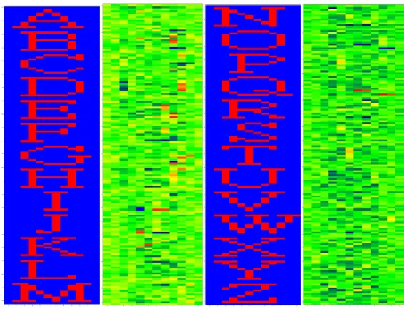
Fig. 2.4 Some English alphabet figures used in this example. ...18

Fig. 2.5 The learning curve of the perceptron ANN for the 26 alphabet letters. ...19

Fig. 2.6 The Confusion matrix (X: Output Y: Desired Output). ...19

Fig. 2.7 The matrix of weighting coefficients (in its origin form)...21

Fig. 2.8 English alphabets and the corresponding reshaped weighting matrices. ...21

Fig. 2.9 Configuration of a back-propagation artificial neuron network...23

Fig. 2.10 Learning curve of a back-propagation ANN with different number of hidden nodes. ...26

Fig. 2.11 The input-to-output characteristic curve of the back-propagation ANN with (a) the training data and (b) the test data. ...27

Fig. 2.12(a) The learning curves of an ANN used for time series prediction. During the learning phase, the data prepared for training the ANN is single, two serial numbers, three serial numbers, respectively. ...28 Fig. 2.12(b) The learning curves of an ANN with different number of hidden nodes.29 Fig. 2.13 The time series (top) and the input-to-output characteristic curves (bottom)

(9)

of a back-propagation ANN with the training data (left) and the test data (right).... ...29 Fig. 3.1 The schematic showing the training process of a back-propagation artificial neuron network. The input data to the ANN is prepared from the SHG Spectrum generated by a coherent pulse with a Gaussian amplitude profile and a desired phase profile...35 Fig. 3.2 Typical training data prepared for the BP ANN. The data comprises the

spectrum and the spectral phase of the coherent pulse under study...36 Fig. 3.3 The resulting SHG spectrum obtained from the training data shown in Fig.

3.2. 37

Fig. 3.4 The curves showing the relation of the population number with r > 0.9 in 1000 data points with the number of hidden nodes in the BP ANN. ...38 Fig. 3.5 This figure show the distribution of r of the case of hidden node number 32 with 1000 test sample and training data...39 Fig. 3.6 L2, L3, L4, L5, L6: the Legendre polynomials of order 2 to 6. ...40 Fig. 3.7 Six SHG spectra are prepared by including more Legendre polynomials in the spectral phase. ...41 Fig. 3.8 The data-flow schematic for the BP ANN training. Six SHG Spectra as shown in Fig. 3.7 were used...42 Fig. 3.9 The curves showing the plot of the population number with r > 0.9 in 1000 data points as a function of the number of hidden nodes in the BP ANN. ...43 Fig. 3.10 A representative phase profile retrieved from the BP ANN with r>0.9 is

plotted to reveal the close agreement with the target phase profile. ...44 Fig. 3.11 Proposed Experimental setup. ...45 Fig. 4.1 An image of 10 bright spots prepared for training the artificial neuron

network localization model...50 Fig. 4.2 One of the images with 25x25=625 pixels and containing single bright spot, used for training the artificial neuron network localization model...51 Fig. 4.3 The distribution of the localization error deduced from a run with either 1000 training images or 1000 test images. ...51 Fig. 4.4 Distribution of the peak position of light spot taken from 1000 training data over an image area of 25x25 pixels. ...53 Fig. 4.5 One of the training images with 11x11 pixels and single bright spot. ...54 Fig. 4.6 Distribution of the peak position of light spot taken from 10000 training data over an image area of 11x11 pixels...55 Fig. 4.7 The distribution of localization error taken from either 1000 training data or 1000 test data after the ANN has been trained for 7500 epochs...56 Fig. 4.8 Comparison showing the localization time of our ANN localization model

(10)

and the 2D Gaussian profile fitting method as a function of the number of spots. ...57 Fig. 4.9 Images showing the influences of noise on the training data. The noise level is set to be 0%, 10 %, 20 % , 30%, 40% and 50 % of the peak height (from top left to right bottom), respectively...58 Fig. 4.10 The distribution of localization error taken from 1000 most populated test data among the set of 10000 data used in our ANN model. The test data are affected by noise with 10%, 20%, 30%, 40%, and 50% of peak height...59 Fig. 4.11 The average localization error as a function of noise level in the test data...

...59 Fig. 4.12 The distribution of localization error taken from 1000 most populated test data among the set of 10000 data used in the 2D Gaussian fitting method. The test data are affected by noise with 0%, 10%, 20%, 30%, 40%, and 50% of peak height. ...61 Fig. 4.13 The distribution of localization error taken from 1000 most populated test data among the set of 10000 data used in the 2D Gaussian fitting method. The test data are affected by noise with 30%, 40%, and 50% of peak height. ...61 Fig. 4.14 An image of 10 bright spots in a size of 256x256 pixels prepared for testing the artificial neuron network localization model. ...62 Fig. 4.15 The target positions (red circles) and the positions (black dots) retrieved

with our ANN localization model. ...63 Fig. 4.16 The same run as Fig. 4.15 except that the test images are affected with

(11)

Chapter 1 General Introduction

1

1 .

.

1

1 F

F

u

n

d

a

m

e

n

t

a

l

P

r

i

n

c

i

p

l

e

o

f

O

p

t

i

c

a

l

M

e

t

r

o

l

o

g

y

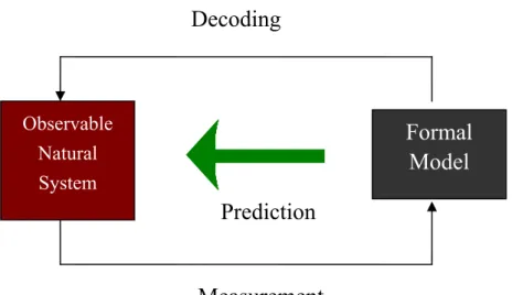
In the field of optical metrology, two fundamental issues encountered are: how to characterize the light to be used, and how to measure the optical signal to extract the information of the measurement. As shown in Fig. 1.1, by analyzing the difference between the intrinsic properties of the light source used and the optical signal from the object under test, the information of the object can be revealed. By analyzing the data we can further construct a model to explain the behavior of the object. After this model is refined with improved knowledge from the data analysis, we can use to model to predict the object behaviors which are still unknown to researchers. In a more aggressive attitude, researchers or engineers can invoke the knowledge accumulated to control or produce the desired response of a physical system by applying a proper waveform of stimulant on the system.

(12)

Fig. 1.1. The schematic showing the relationship of measurement, model construction, and the control of a physical system.

The fundamental properties of a light field including the amplitude, phase (revealing via frequency or wavelength), and the state of polarization can be invoked in optical metrology. For examples, as illustrated in Figure 1.2, the amplitude of an optical field can be modified by a material and the information can be used to reveal how much light energy is absorbed as the light beam passes through the medium, which relates to the band structure of material. Furthermore, by detecting the frequency shift of a light field as it reflects from a moving object, we can deduce the information about the velocity of the object, which is known as the Doppler Effect. The direction and the state of polarization of a light field after passing through a transparent medium such as a thin film of liquid crystal will be changed and the polarization variation carries the information about the orientational profile of the liquid crystal molecules in the film.

Measurement

Formal

Model

Observable Natural System

Decoding

Prediction

(13)

Fig. 1.2. Examples showing the information of physical properties of a medium can be embedded in the three fundamental characteristics of a light field.

Among a variety of the light-matter interaction processes such as optical absorption by crystalline silicon, the absorption of an incident photon with energy larger than the band gap of the medium can readily create an electron-hole pair and results in photocurrent. As the strength of the optical field increases, numerous nonlinear optical

Frequency shift of a light field after reflecting from a moving object Light amplitude is decreased due to an absorption of photon by matter.

(14)

one can tightly focus the light beam on a medium with a field-concentrating tip, the signal to be detected will mainly originate from the illuminated area under the tip. By using such a tip, we can achieve an extremely high spatial resolution beyond the optical diffraction limit. On the other hand as shown in Fig. 1.3, if one can employ optical pulses with duration down to a few femto-seconds to probe a medium, the deep insight into the ultrafast dynamics of the excited medium may be yielded. When optical pulses with ultra short duration are used for probing materials, dynamic studies of materials, such as the dynamic processes of a chemical reaction, photosynthesis, interaction between proteins and substrates, photo-excited electron-hole relaxation, shall become possible. However, to realize the potential of optical metrology at the femtosecond scales, techniques that can be employed fully characterize the ultrafast light field must be developed. Conduction band Valence band λ λ I T

Fig. 1.3. Schematic showing an optical absorption process of broadband light by a medium. The information about the band structure of the medium and the dynamics of light-matter interaction can be embedded into the dynamic spectrum of the light after passing through the medium.

(15)

A proper characterization of the light field to be used in ultrafast optical metrology is not a simple task. In the past few decades, several methods had been developed in order to solve the issue. Optical intensity autocorrelation (AC) [1] is the first technique to deduce the temporal profile of a laser pulse. Although the autocorrelation can yield pulse information in time domain, the profile deduced is not the real field profile of the optical pulse. Furthermore, the biggest disadvantage of the technique is that it carries no information about the phase of the optical pulse. To fully characterize an optical pulse field, several two-dimensional methodology such as frequency-resolved optical gating (FROG) [2] and spectral phase interferometry for direct electric-field reconstruction (SPIDER) [3] had been developed in the past two decades. The schematic setups of FROG and SPIDER are illustrated in Figs. 1.4.

FROG is similar to the autocorrelation except that it detects the transient spectra of an optical pulse instead of intensity. We use FROG to acquire the spectra with different time delays and assemble a time-frequency distribution of the pulse. We then retrieve the phase information from the time-frequency distribution by using an iteration algorithm. SPIDER is based on the concept of spectral-shearing interferometer; the optical pulse to be measured is split into two parts, with the time delay and phase delay to be adjusted separately. And then the two parts of the pulse can be recombined to generate a set of fringe patterns. The major advantage of SPIDER is that the set of fringe

(16)

patterns can be used to retrieve the spectral phase of the pulse field in a direct way without invoking any iteration procedure. Therefore, the information retrieving speed from data of SPIDER can be very fast.

Detector used in AC: power meter; FROG: spectrometer. Detector BS Mirror _LEN BS BS BS LEN SLM LEN Spectrometer

Fig. 1.4. Typical experimental setup for frequency resolved optical gating (FROG, top) and spectral phase interferometry for direct electric-field reconstruction (SPIDER, bottom).

(17)

To characterize the structure of a heterogeneous material such as the organization and distribution of molecules or subcellular objects in a cell raises the need to precisely localize these objects. The position and velocity of a nano object can be determined by localizing the corresponding light spots in a 2D photo-detector in an optical microscope. By tracing the particle in real time, important mechanisms in a live cell had been revealed. The light spots can be originated from either light scattering or fluorescent emission from nanoparticles. The technique that can accurately localize nano particles is also an important tool in the material structural determination, especially for nanostructured materials.

To localize nanoparticles with the nanometer accuracy, we first have to excite the particles at very low level such that two light spots from neighboring excited particles

Fig. 1.5. Schematic shows the concept of concentrating the light field on a medium with a tip. The signal to be detected will mainly originate from the illuminated area under the tip, yielding the possibility to localize particles with high spatial resolution.

(18)

the optical microscope used. The central positions of the light spots are then fitted to 2D Gaussian profiles [4] or with the center-of-mass method. The fitting of a light spot to a 2D Gaussian function in principle can determine the sub-pixel center of the light spot. Unfortunately, the localization accuracy with the method is time consuming and sensitive to the signal-to-noise ratio of the data.

For the center-of-mass method, the center-of-mass of a light spot can be calculated as the weighted position of all pixels involved in the spot. For the case shown in Fig. 1.6, the mean value can be (1*1+2*2+3*2.5+4*1)/(1+2+2.5+1)=2.5385.

0 0.5 1 1.5 2 2.5 3 1 2 3 4

1

1 .

.

2

2 O

O

v

e

r

v

i

e

w

o

f

A

r

t

i

f

i

c

i

a

l

N

e

u

r

a

l

N

e

t

w

o

r

k

An Artificial Neural Network (ANN) [5] is an algorithm designed to simulate the capabilities of learning and data processing of the neuron network in our brain. ANN

(19)

simulates our brain on two aspects; firstly, the knowledge learning from the data can be updated and stored in the weighting parameters of ANN. Second, the set of optimal weighting parameters can be deduced through a learning process. The schematic of the overall process is depicted in Fig. 1.7. The input data is first converted into an output, and then the calculated output is compared with the desired output to generate an error, which can be feedback to adjust the weighting parameters of ANN in order to further reduce the error. By this way, the output can approach the desired performance.

ANN can be invoked to offer several useful functionalities, including data classification, functional approximation, and series prediction, etc. [6-8]. Usually, one can start with data analysis, and then based on the results to construct a preliminary model. After testing and verification involved in the learning process, the trained ANN

Input Output

Desired Output Error Error feedback to

adjust weight of ANN

ANN

(20)

the data is complex and cannot yield sufficient information to expose the underlying structures, ANN could be very valuable in this case.

1

1 .

.

3

3 M

M

o

t

i

v

a

t

i

o

n

a

n

d

O

u

t

l

i

n

e

o

f

t

h

i

s

T

h

e

s

i

s

In this thesis, we will apply ANN for producing an intelligent learning system to improve the measurement accuracy or generating new functionality of an apparatus in optical metrology, namely the complete characterization of ultrashort laser pulses and nanometer localization in real time for an optical microscope. The techniques needed to implement artificial neuron network for the two applications will be developed.

We also like to implement the learning ability of artificial neuron network into an optical apparatus to accumulate the user experiences and improving the prediction accuracy of the ANN as more data are taken. To achieve this goal, this thesis is organized as follows:

In chapter 2, we will first review the general concepts of ANN and introduce the skills needed for the applications. We will introduce the most useful functionalities of ANN, some illustrative application examples are prepared too.

In chapter 3, we will combine ANN with a second-harmonic generation spectroscopy to retrieve the spectral phase profile of ultrashort optical pulse field and yield the complete field information of the pulse. Feasibility of this application is

(21)

demonstrated and difficulties encountered are discussed.

In chapter 4, we will develop an ANN scheme to search and locate the position of particles with an optical microscope. The feasibility of artificial neuron network to find the central position of a light spot was revealed. Higher accuracy, faster localization process and more immune to the noise than that does by the 2D Gaussian fitting were demonstrated.

(22)

Chapter 2 Introduction to Artificial Neural Network

In Section 2.1, we review the development history and some background of artificial neural network. We will describe how does the artificial neural network work in Sections 2.2 to 2.4 and then present application examples to illustrate the important functionalities of ANN, including classification, functional approximation and time series prediction. A brief summary will be given in Section 2.5.

2.1 Overview of Artificial Neural Network

2.1.1 Historical Development of ANN

Inspired by the structure of neuron and the connection topology in brain, the first mathematical model of neural network was reported in 1943 by Warren McCulloch and Walter Pitts [9]. In 1958, Frank Rosenblatt developed the first practical network with related learning rules, which is now named as the artificial neural network structure of perceptron [10]. From 1967-1982, Marvin Minsky and Seymour Papert discovered some limitations of existing neural networks [11], such as that ANN cannot perform some complex logical operations for example XOR, and new learning algorithms were not put forward causing researches to suspect the limited functionality of ANN. However, the development stagnation of ANN finally broke in 1980s. Several new architectures of

(23)

ANN and theorems had been discovered, including the self-organizing map structure by Teuvo Kohonen in 1982 [12], the Hopfield neural network by John J. Hopfield in 1983 [13], and David Rumelhart’s group reported back-propagation neuronal network in 1986 [14]. Furthermore, in 1991 Stephen Grossberg developed the adaptive resonance theory [15] that can significantly improve the learning capability of an artificial neural network. Thanks to these progresses, artificial neural network has been widely used in the pattern recognition, identification, and data classification.

Hossein reported in 1989 [16] that if the weights of a backward-propagating ANN are initially set to be high values, the learning performance of the ANN will be improved and the best initial values depend on the problem. Kruschke [17] inserted a gain into a backward propagation network and found a regularization effect on the weights, which improves the performance of backward ANN. Sarker [18] found by tuning the weights the oscillation occurring in ANN can be reduced. Kubat [19] used a determination tree to guiding the construction of a backward-propagating ANN. Wu [20] developed a method of optimizing the hidden layers’ outputs (OHLO) to isolate each neural layer and then to modify the weights and inputs. Leung [21] combined the weight evolution method with a new generalized back-propagation method to accelerate the convergence and avoid the problem of trapping into a local minimum.

(24)

2.1.2 Technical Background of ANN

Artificial neural network is an algorithm that simulates the function of brain. In order to make an artificial neural network function properly, the algorithm must be divided into two major steps: the first step is called a learning phase and the second step is a retrieving phase. In the learning phase, we need to adjust the system parameters of an artificial neural network such as weights or bias. In the retrieving phase, we can use the artificial neural network to predict the result based on new input data.

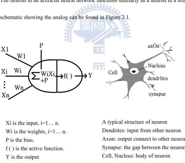
The neuron in an artificial neural network functions similarly as a neuron in a brain. The schematic showing the analog can be found in Figure 2.1.

Xi is the input, i=1… n. Wi is the weights, i=1… n. P is the bias. f ( ) is the active function. Y is the output

Fig. 2.1. Schematic shows the analog of artificial neuron and brain neuron structure. A typical structure of neuron

Dendrites: input from other neuron Axon: output connect to other neuron Synapse: the gap between the neurons Cell, Nucleus: body of neuron

(25)

As shown in Fig. 2.1, the {Xi}, i=1,…,n denotes an excitation from other neuron, and {Wi}, i=1,…,n represents a set of weighting coefficients denoting the connection strength between neurons, P denotes a threshold level beyond which a neuron will fire. And Y is the excitation to other neurons. Depending on the performance desired, a variety of active functions have been adopted in different artificial neural networks. Several useful forms of active function are step function, sign function, hyperbolic tangent function, or sigmoid function, which is defined as

1 1 x b

Sigmoid

e 



 , Hyper tangent tanh( x b ). b: the intercept on x axis. (2-1)

Step function Sign function

Hyper tangent Sigmoid

(26)

2.2 Typical Structures of ANN and the Corresponding Application

Examples

2.2.1 The Perceptron Architecture

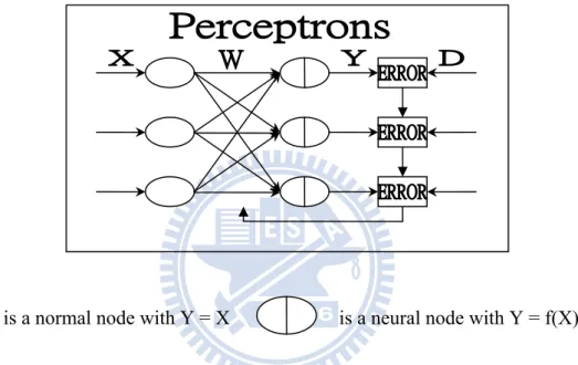
Perceptron is the first practical ANN, typically used for data classification. Figure 2.3 shows the structure of a perceptron with a structure of input layer and output layer.

is a normal node with Y = X is a neural node with Y = f(X)

Fig. 2.3. A typical perceptron structure

A perceptron ANN usually uses either a step function or a sign function as its active function depending on the training data set used. Denoting Xi to be the input of

the i-th input node, Wij the weighting coefficient the i-th input node and the j-th neural

node, then the input of the j-th neural node can be expressed as

1 N j i ij j i Y X W P  



 . Here

N is the total number of input nodes, Pj is the bias of the neural node, and Yj is the output

(27)

between Yj and Dj. We can use E to adjust the ANN system parameters Wij and Pj by

following the learning rule shown below: ( 1) ( ) ij ij j i W t W t E X (2-2) ( 1) ( ) j j j P t P t E , (2-3)

where η denotes the learning rate with a typical magnitude ranging between 0 and 1, Ej

= Dj – Yj, and t is the iterations.

The training process can be set up by dividing the process into the following steps: 1. First, random numbers between zero and one are used to initialize the weighting

coefficients and biases.

2. An input data pattern is inserted at the input, and the output and related errors E are calculated.

3. Using the errors and the learning rules to update the weighting coefficients and biases.

4. Repeat the steps 2 and 3 until the desired result is achieved with a satisfactorily small error.

2.2.2 Application Example of Perceptron

In this section, we will apply a perceptron for data classification to illustrate how this network works. The application example is to classify the 26 English alphabets. The

(28)

26 English alphabets were presented in a figure format of 12x12 pixels figure at the input of the perceptron. Figure 2.4 presents some of the letter figures. The output of the ANN is shown by an array of twenty six digits such that the output of alphabet A is (100000…0), B is (010000…0), C is (001000…0)…etc.

Fig. 2.4. Some English alphabet figures used in this example.

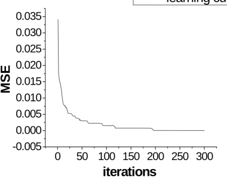
We converted each alphabet figures (from first to the last pixel) into an integer array of 144 elements and used the array for the input data. If the pixel is black, the corresponding integer is one. Otherwise it is zero. We therefore have 26 input data sets with each data being one dimensional array of 144 components of ones or zeros. For the output, we use a 26x26 identity matrix with each row corresponding to the desired output, resulting in a perceptron of 144 input neurons and 26 output neurons. The learning rate is set to be 0.5. The weight coefficients are set to be 0.25 by adjusting the bias. As the result, the learning process can converge with a learning curve shown in Fig. 2.5, indicating that the mean square error (MSE) can approach zero. As shown in Fig. 2.6, the ANN can successfully recognize the alphabet letters with an extremely low

(29)

0 50 100 150 200 250 300

-0.005

0.000

0.005

0.010

0.015

0.020

0.025

0.030

0.035 M

S

E

iterations

learning curve

Fig. 2.5. The learning curve of the perceptron ANN for the 26 alphabet letters

(30)

The learning curve is different for each training cycle of the alphabet letters because the initial weighting coefficients are generated by random number generator and they are of course different for each training cycle. Nevertheless, the final results with different initial set of weighting coefficients are similar.

The weighting coefficients and biases can be represented by matrices with the dimensions of 144x26 and 26x1, respectively. Fig. 2.7 presents the original matrix form of weighting coefficients. Fig. 2.8 shows the reshaped form of the weighting matrix with dimension of 12x312 with the weighting coefficients at the same pixel position in each alphabet letter figures. It was found that the weighting coefficients have large magnitudes at the positions corresponding to the positions of the black pixels in the alphabet letter figures. The weighting coefficients with larger magnitudes reveal those important pixels in the alphabet letter figures. The ANN after training may invoke those pixels to recognize the characteristic features of the alphabet letters. We found that those important pixels are clustered in the central region.

(31)

Fig. 2.7. The matrix of weighting coefficients (in its origin form).

Fig. 2.8. English alphabets and the corresponding reshaped weighting matrices

For example, if an ANN tries to distinguish the alphabets O from X. It may firstly examine the pixels locating at the central region of the letters to find some important

(32)

not be the only way to distinguish. There may have several possible forms of weighting matrix to meet our goal. The weighting matrix, which yields a power of recognition, is a solution to an equation that connects the desire output vector to the multiplication of the input vector and the weighting matrix. Since there are 26 alphabet letters, we have a set of linear equations with 144x26 variables and 26x26 constraints. It is not surprising that many solutions may exist. In the case that the equations do not have a solution, the training process would fail and no satisfied weighting matrix could be produced. Although a perceptron structure is suited for data classification and recognition, it cannot be used for function approximation. Researchers in the past had developed another type of ANN structure, called back-propagation neuron network to expand the applicability of ANN.

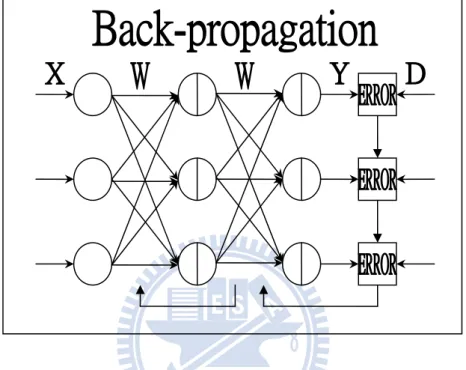
2.2.3 Back-Propagation Artificial Neuron Network

Back-propagation artificial neuron network is useful in many applications of ANN. The typical structure of a back-propagation ANN is illustrated in Figure 2.9, which has a multilayer configuration. Here W is the matrix of weighting coefficients of the ANN. For using an input data X, the ANN can generate an output Y with the desired output D. Back-propagation ANN typically possesses a structure of three to four layers, including one input layer, one output layer and one or two hidden layers. The active function

(33)

implemented in back-propagation ANN is sigmoid function in both hidden layers and output layer to enhance the performance in the learning phase with nonlinear data structure.

Fig. 2.9. Typical configuration of a back-propagation artificial neuron network

The learning procedure of a back-propagation ANN is summarized as follows: Firstly, the input data and the corresponding desired output are sent to the ANN. The input data propagates forward layer by layer from the input layer, hidden layers to the output layer. The resulting error, which is defined to be the difference between the output and the desired response, is calculated. The weighting coefficients and biases of the ANN are then adjusted in order to minimize the error. Because the ANN has a multi-layer structure, we need to invoke chain rule to calculate the gradient of the

(34)

system parameters used in the error function.

The learning rule of back-propagation ANN is described as follows. We denote Wjk

to be the weighting coefficient between the j-th hidden neuron and the k-th output neuron. The bias of the j-th hidden neuron and the k-th output neuron is denoted as Pj

and Pk, respectively. Yk is the output from the k-th output neuron with Dk the desired

output, and Hj is the output from the j-th hidden neuron. Therefore, Yk and Hj can be

given by 1 ( n ) ( ) j i ij j j i H F X W P F net  



  (2-4) 1 ( ) ( ) m k j jk k k j Y F H W P F net  



  . (2-5)

Here F is the active function. The sum of the variables in the active function is defined as a new variable “net”, and n and m are the number of input neuron and the number of hidden neuron, respectively. Error function will be defined as

2 1 1 ( ) 2 l k k k E D Y  



 , (2-6)

where l is the number of output neuron.

We used the gradient descent algorithm to minimize the error function, leading to the following equations to be used for adjusting the weighting coefficients and bias parameters. ( 1) ( ) jk jk jk E W t W t W       , (2-7) ( 1) ( ) k k E P t P t P       , (2-8)

(35)

where t is the iterations and η is the rate constant of learning process.

By using the chain rule, we can calculate the partial derivatives in Eqs. 2.7 and 2.8, which lead to (detail in appendix I)

( 1) ( ) jk jk k j W t W t  H , (2-9) ( 1) ( ) k k k P t P t  , (2-10)

where (_k  D_k Y F net_k) '( _k), let _k be the error of the k-th output neuron and we can use _k to adjust the bias at the nodes in the hidden layer and the weighting coefficients between input layer and hidden layer by

( 1) ( ) ij ij j i W t W t  X , (2-11) ( 1) ( ) j j j P t P t  , (2-12) where 1 '( _j) l _k _jk k j F net W   





. Because the active function used is a sigmoid function, we can simplify F net'( j) to a multiplication of sigmoid functions as shown below

1 1 1 ( ) ( )(1 ) ( )(1 ( )) 1 x 1 x 1 x d d F x F x F x dx dx e  e  e   . (2-13)

Eqs. 2-10 and 2-11 form the basis of learning needed to train the ANN.

2.2.4 Application of Back-Propagation Artificial Neuron Network for Function

Approximation

The function approximation is the most useful feature of ANN. This functionality of ANN can be use to approximate the relationship between input and output of a

(36)

physical system. Here we consider a simple application example of back-propagation ANN to approximate the relationship between the critical angles of the interface between two media, which is known as the Snell’s law. The critical angle of light passing through an interface of two media is known to be

1 1 2

sin ( / )n n



_  _, _(2-13)

where n ,₁ n are the refractive indices of the two medium. For this case, we construct a ₂

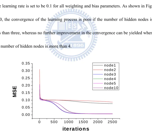
back-propagation ANN with two input nodes, four hidden nodes and one output node. The learning rate is set to be 0.1 for all weighting and bias parameters. As shown in Fig. 2.10, the convergence of the learning process is poor if the number of hidden nodes is less than three, whereas no further improvement in the convergence can be yielded when the number of hidden nodes is more than 4.

0 5 0 0 1 0 0 0 1 5 0 0 2 0 0 0 2 5 0 0 0 .0 0 0 .0 5 0 .1 0 0 .1 5 0 .2 0 0 .2 5 0 .3 0 0 .3 5

MSE

ite ra tio n s

n o d e 1 n o d e 2 n o d e 3 n o d e 4 n o d e 5 n o d e 1 0

Fig. 2.10. Learning curve of a back-propagation ANN with different number of hidden nodes.

(37)

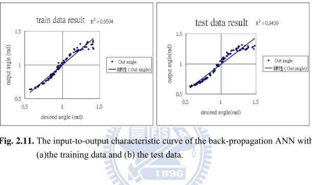
After training, the ANN can simulate the training data and predict the test data as shown in Figure 2.11. The predicted values of ANN agree very well with the theoretic curve.

Fig. 2.11. The input-to-output characteristic curve of the back-propagation ANN with (a)the training data and (b) the test data.

2.2.5 Application of Back-Propagation Artificial Neuron Network for Time Series

Prediction

Time series prediction is useful for the prediction of weather temperature, the periods of sunspot, and chaos, etc. Time series prediction is very similar to functional approximation. Here we will focus on the issue of how to use ANN to predict the behavior of a chaotic series. We created a chaotic series with the follow formulas:

0 1 0.01 4 (1 ) t t t Y Y_ Y Y    , (2-14)

(38)

For time series prediction, the input to an ANN is the data we have prepared. For example, we can use Y1 to Y3 from Eq. 2-14 as the input data and Y4 as the desired output

of the ANN. Similarly, we can shift one position and take Y2 to Y4 as the input and Y5 as

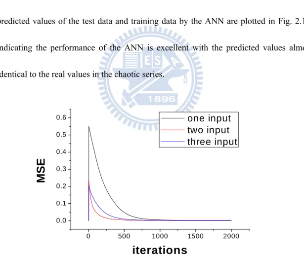
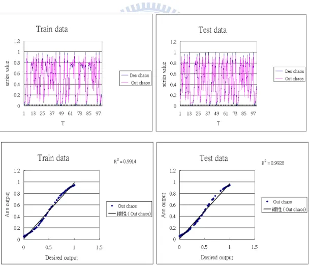
the desired output. In this way, we can prepare numerous dataset to train the ANN. We chose the learning rate to be 0.01 for all weighting and bias parameters. The learning curves with different sets of system parameters are presented in Figure 2.12. After training, we can use the ANN to predict the data remaining in the time series data. The predicted values of the test data and training data by the ANN are plotted in Fig. 2.13, indicating the performance of the ANN is excellent with the predicted values almost identical to the real values in the chaotic series.

0 500 1000 1500 2000 0.0 0.1 0.2 0.3 0.4 0.5 0.6

MSE

iterations

one input two input three input

Fig. 2.12(a) The learning curves of an ANN used for time series prediction. During the learning phase, the data prepared for training the ANN is single, two serial numbers, three serial numbers, respectively.

(39)

0 500 1000 1500 2000 0.0 0.1 0.2 0.3 0.4 0.5 0.6

Error

iterations

h1

h5

h10

Fig. 2.13. The time series (top) and the input-to-output characteristic curves (bottom) of a back-propagation ANN with the training data (left) and the test data (right). Fig 2.12(b) The learning curves of an ANN with different number of hidden nodes.

(40)

2.3 Summary

From the case studies shown in this chapter, we found that ANN is useful for numerous applications. Most of the applications of ANN use the back-propagation structure. Function approximation is useful to simulate the behavior of a physical system, which the underlying processes inside the system are unclear. We can build an ANN to simulate the relationship between the input and output of a physical system. The most sensitive issue of ANN relates to the training process. The training process requires much CPU time and may yield poor performances if an inappropriate ANN structure is implemented and is trained with inappropriate data sets.

(41)

Chapter 3 Complete Characterization of Ultrashort

Coherent Optical Pulses with SHG Spectral

Measurement

3.1 Introduction

As explained in Chapter 1, the complete field characterization of coherent optical pulses is the first step to invoke these optical pulses for optical metrology. Several techniques had been developed to offer the complete characterization of coherent optical phases, such as frequency-resolved optical gating (FROG) first reported by D. Kane and R. Trebino [2], and spectral-phase interferometry for direct electric field reconstruction (SPIDER) developed by T. Tanabe, et al. [3].

The basic concept of FROG is quite similar to the autocorrelation measurement but FROG measures the spectrums at different time delays instead of optical intensity only. Retrieving the spectral phases and then yielding a complete-field information of the coherent pulse under study is via an iteration algorithm. SPIDER can directly measure the spectral phase of a coherent pulse with a spectral-shearing interferometer, which separates the incoming coherent pulse into two parts and sent one part through a linear spectral phase modulator, and the other through a linear temporal phase modulator. And then by superpose these two parts together to yield a spectral-shearing interferogram.

(42)

The spectral phase and therefore the complete field information of the coherent pulse can be deduced directly from the interferogram without involving any further iterative calculation.

Along the development of complete coherent pulse characterization, Dorrer, et al. had invoked a self-referencing device based on the concept of shearing interferometry in the space and frequency domains to perform the spatio-temporal characterization of ultrashort light pulses [22]. Weiner et al. [23] had demonstrated the spreading of femtosecond optical pulses into picosecond-duration pseudo-noise bursts. In this case, pulse spreading was accomplished by encoding pseudorandom binary phase codes onto the optical frequency spectrum. Subsequently, decoding of the spectral phases restores the original pulse. Shelton et al. have generated a coherently synthesized optical pulse from two independent mode-locked femtosecond lasers, providing a route to extend the coherent bandwidth available for ultrafast science [24]. Applications of coherent light pulse characterization techniques in femto-chemistry had been well reviewed in [25].

Another attractive approach to characterize coherent laser pulse is to use an adaptive feedback-controlled apparatus to tailor the spectral phase of a coherent pulse to achieve the maximum second harmonic generation output from a nonlinear optical crystal [26]. In this way, the compensating spectral phases carry the spectral phase information about the coherent pulse under study.

(43)

Control the quantum evolution of a complex system is an important advance in optical metrology. The technique has now been coined as coherent or quantum control. Adaptive coherent pulse control [27-30] is the most successful scheme to be used for quantum control. Several algorithms have been developed to tailor a coherent optical field for a specific target on the basis of fitness information [31-36]. In this regard, a freezing phase concept had been proposed for adaptive coherent control with a femtosecond pulse shaper [26].

Our main goal of this study is to develop an artificial neuron network (ANN) model which can be used to retrieve the spectral phase of a coherent pulse directly from the spectrum of the second harmonic generation (SHG) with a nonlinear optical crystal. The SHG spectrum is affected by both the SHG process and the spectrum of the incident light pulse. In this chapter, we will develop an ANN to help us retrieving the spectral phase and therefore the complete-field information of a coherent pulse (phase and spectrum) with the measured spectrum of second harmonic generation.

Assuming the temporal profile of a coherent pulse is known, therefore we only need to adjust the spectral phase of the input pulse to generate the maximum SHG output from a nonlinear crystal. From the measured SHG spectrum, we retrieve the spectral phase of the input coherent pulse with an artificial neuron network. If the approach is successful, we can simply retrieve the complete field information of a

(44)

coherent pulse in real time directly from a measured SHG spectrum without time-consuming computation. The apparatus needs only NLO (Nonlinear Optics) crystal and a spectroscope.

3.2 Theory

Considering an incident coherent optical pulse ( ) ( ) i ( )

E



 A



e  with a spectrum of A w( ) and spectral phase distribution of j w( ). The second harmonic generation spectrum can be expressed as

2

(2 )

(

)* (

)

SHG

I

 



E



 

E



  

d

. (3-1)

Assuming the spectrum of the coherent pulse to be Gaussian, and the spectral phase profile can be properly depicted with a polynomial of order 6, usually factor the phase of a high order is much small than the low order we cut it off at the order six.

2 2 0

( ) exp(

/

)

A







 

, (3-2) 6 0

( )

n n n

a

 







_. _(3-3)

In general, the phase terms of order zero and one do not have any effect on SHG. The spectral phase profile can be further simplified by including terms from two to six only.

Note that from the point of view of theory, it shall be impossible to retrieve the spectral phase of a coherent pulse directly from the SHG spectrum of a coherent pulse. Therefore, in the following we will conduct some simulations to test the feasibility of

(45)

3.3 Simulation 1

3.3.1 Preparation of the training data set

To prepare the training process of ANN, we sampled the spectrum and phase of a coherent Gaussian pulse to generate 64 data points. The second harmonic spectrum is presented with a data array of 127 data points because the second harmonic spectrum was calculated via a convolution operation.

The schematic of the training process is detailed in Fig 3.1. The input into a back-propagation artificial neuron network is the data of the second harmonic generation pulse comprising a spectral profile array and a spectral phase array.

Fig. 3.1. The schematic showing the training process of a back-propagation artificial neuron network. The input data to the ANN is prepared from the SHG Spectrum generated by a coherent pulse with a Gaussian amplitude profile and a desired phase profile.

BPANN _Error

Desired Phase SHG Spectrum

(46)

3.3.2 Creation of a Backward Propagation Artificial Neuron Network

The input layer of the BP ANN was designed to accommodate the 127 inputs of the second harmonic generation spectrum. The output layer generates the retrieved spectral phase profile for the coherent pulse under study. A typical training data for the coherent pulse under study is shown in Fig. 3.2. The resulting SHG spectrum obtained from the training data is presented in Figure 3.3. We had investigated BP ANN with different numbers of hidden nodes and different learning parameters to find out the best learning performance of the artificial neuron network. The results will be discussed in the following section.

0

10

20

30

40

50

60

70 -5

0

5

10

15

20

25 Ph

ase (rad

)

Pixel

Amp

Phase

Fig. 3.2. Typical training data prepared for the BP ANN. The data comprises the spectrum and the spectral phase of the coherent pulse under study.

(47)

0

20

40

60 80 100 120 140

0.00

0.01

0.02

0.03 I (a.u.)

pixel

SHG

3.3.3 Results and Discussion of Simulation 1

In this simulation, we used a two-layer BP ANN to find out how many hidden nodes are needed to yield a satisfactory learning performance. The active function of each node was chosen to be the sigmoid function and the rate constant of learning rate was set to be 0.1 for the first and the second weighting layers. In the learning phase, we trained the network by 1000 epochs. To evaluate the performance of the training, we used a correlation coefficient r, which is define as

x y x y S r S S  . (3-4)

Fig. 3.3. The resulting SHG spectrum obtained from the training data shown in Fig. 3.2.

(48)

Here , 1 1 ( )( ) 1 n x y i j i j S x x y y n    





, and Sx, Sy are the standard deviations of x, y.

The correlation coefficient can reveal the underlying relation between two sets of data. It value lies between -1 and 1 with value one implies a prefect linear dependence. In our case, r=1 means the output of the ANN is same as the desired output.

0 10 20 30 40 50 60 70 220 240 260 280 300 320 340 360 380 400

Num.

of sampl

e r > 0.

9 Hidden Node Num.

Test Set

Data Set

Figure 3.4 presents a plot of the population number with r > 0.9 in 1000 data points as a function of the number of hidden nodes used in the BP ANN. We can find that by increasing the number of hidden nodes the number of data points with the correlation coefficient higher than 0.9 increases, implying that the predicted values with ANN can

Fig. 3.4.The curves showing the relation of the population number with r > 0.9 in 1000 data points with the number of hidden nodes in the BP ANN.

(49)

increasing tendency becomes stagnated. Therefore, the best choice is a BP ANN with each hidden layer containing about 20 hidden nodes.

-1.0 -0.8 -0.6 -0.4 -0.2 0.0 0.2 0.4 0.6 0.8 1.0 0 50 100 150 200 250 300 350 400

Num. of sample

r

data

test

From the distribution of r presented in Fig 3.5, we found that only about 35% of the predicted values of spectral phase has a correlation coefficient higher than 0.9. Apparently, the learning performance of this SP ANN is not satisfactory. In view that the spectral phases used are expressed in terms of polynomials, we may be able to solve the problem with an increase of the information content in the training data by including more orthogonal phase profiles. Therefore, in the next section, we will try to express the spectral phase profile in terms of Legendre polynomials of order 2 to 6, which are shown

Fig. 3.5. The resulting distribution of r with 1000 test data points , and 1000

(50)

in Figure 3.6.

0

10

20

30

40

50

60

70 -8

-6

-4

-2

0

2

4

6

8 L2

L3

L4

L5

L6

P

h

ase (rad)

Pixel

3.4 Simulation 2

3.4.1 Preparation of the Training Data Set

Legendre polynomials form a complete set of orthogonal basis for a continuous function. By expanding the spectral phase profile of a coherent pulse into Legendre polynomials, we can significantly increase the information content with a minimum number of Legendre polynomials. Indeed as shown in Fig. 3.7, by including Legendre polynomials of order 2 to 6 in the spectral phase profilej w( ), more complicated SHG spectrum can be synthesized. The method significantly increases the degrees of freedom

(51)

in the phase retrieval procedure. Six SHG spectra are prepared for the training of BP ANN by including more Legendre polynomials in the spectral phase are shown in Figure 3.7.

0

20

40

60 80 100 120 140

0.00

0.01

0.02

0.03 pixel

I (

a

.u.)

No Add

L2 Add

L3 Add

L4 Add

L5 Add

L6 Add

3.4.2 Creation of the Backward Propagation Artificial Neuron Network

For this study, we built another BP ANN which contains 762 input nodes and 64 output nodes. The 762 (6x127=762) input nodes are designated for the six SHG spectrums and 64 output nodes are for the retrieval spectral phase of the coherent pulse under study. The learning rate is set to 0.1 for both the first weighting layer and the second weighting layer. The data-flow schematic for the training is shown as Fig 3.8.

Fig 3.7. Six SHG spectra are prepared by including more Legendre polynomials in the spectral phase.

(52)

3.4.3 Results and Discussion of Simulation 2

The simulation results showing the relation of the population number with r > 0.9 in 1000 data points with respect to the number of hidden nodes in the BP ANN used are presented in Fig. 3.9. The results are quite encouraging in view that the number of the predicted phases with a correlation coefficient r> 0.9 can reach more than 90% of the test samples.

Fig 3.8. The data-flow schematic for the BP ANN training. Six SHG Spectra as shown in Fig. 3.7 were used.

Desire Phase Six SHG spectrums

Error BPANN

(53)

0 10 20 30 40 50 60 70 300 400 500 600 700 800 900

Num. of s

am

p

le r >

0.9 Hidden Node Num.

Test Set

Data Set

We presented in Fig. 3.10 some representative profiles with r>0.9 to give some hints of how well the BP ANN performs. From this Figure, we can see that the phase profile retrieved by our ANN agrees very well with the target profile.

Fig 3.9. The curves showing the plot of the population number with r >

0.9 in 1000 data points as a function of the number of hidden nodes in the BP ANN.

(54)

0

10

20

30

40

50

60

70 -5

0

5

10

15

20

25 Piexl

Phase (rad)

Amp

Target

Retrive

3.5 The Proposed Experimental Setup

For an experimental realization of the technique, one may concern how to conduct the training of BP ANN and then how use the trained ANN to perform the complete field characterization of a coherent pulse experimentally. We proposed an advanced apparatus with a pulse shaper to yield an adaptive feedback control loop as depicted in Fig. 3.11. By using this apparatus, we can first measure the spectrum of the laser pulse under study. We can produce many possible phase distorted versions of the coherent pulse by combining the measured spectrum with a variety of spectral phases expressed as a series

Fig 3.10. A representative phase profile retrieved from the BP ANN with r>0.9

(55)

ANN. After training, the trained ANN can be invoked to retrieve the spectral phase of the coherent pulse with the measured SHG spectrum. The apparatus offers a possibility to perform a complete-field characterization of a coherent excitation and quantum control of a physical system in a single setup.

3.6 Conclusions

We developed a BP ANN which can be invoked to retrieve the spectral phase of a coherent pulse from the measured SHG spectrum. We proposed a setup to be used for the experimental realization of the concept. By using this apparatus, we only need to measure the spectrum of the coherent pulse under study and then combine the spectrum with a variety of spectral phase profiles to prepare the SHG spectra for training the BP ANN. The trained BP ANN can be invoked to retrieve the spectral phase profile for the

SHG crystal Spectrometer Phase Modulator Plus ANN System Phase information Phase retrieve

(56)

the predicted phases can achieve the target profile with more than 90% confidence. Thanks to the computation efficiency of BP ANN, the technique developed in this study offers a possibility to perform a complete-field characterization of a coherent excitation to a physical system and quantum control of the system in a single setup.

(57)

Chapter 4 Real-Time Localization of Nano Objects at

the Nanometer Scales

4.1 Introduction

An isolated fluorescent molecule or nano object will be observed like a light spot under an optical microscope. The spatial profile of the light spot simply reveals the point spread function of the optical microscope used. The peak position of the light spot can be determined with an accuracy of 1 nm if the signal-to-noise ratio of the detection is high enough. This impressive feature of nanometer localization with optical microscopy had recently inspired many applications including Fluorescence Imaging with One Nanometer Accuracy (FIONA) [37], sub-diffraction-limit imaging by stochastic optical reconstruction microscopy (STORM) [38], and fluorescence photoactivation localization microscopy (FPALM) [39], etc. Important biophysical mechanisms at the subcelluar scales had been discovered [40].

In the historical point of view, we noticed that a modified Hough transformation had been developed to detect a circular object [41] for recognizing and classifying interesting features present in a phase-contrast (PC) cytological image. Fillard, et al. had invoked the frequency dependence of the argument of Fourier transform to analyze an in-focus two-dimensional Airy disk [42]. Alexander, et al. proposed a method to

(58)

eliminate the systematic error in centroid estimation and achieved a subpixel accuracy [43]. It is interesting to know that a diffractive optical element (DOE) [44] had been applied to effectively locate a laser spot on a projection screen. The method could be invoked to achieve nanometer localization for optical microscopy. Anderson had presented an algebraic solution to the problem of localizing single fluorescent particle with sub-diffraction-limit accuracy [45]. Qu, et al. [46] had demonstrated nanometer localization of multiple single-molecules (NALMS) by using fluorescent microscopy and photobleaching properties of fluorophores. Cui, et al. [47] had devised an optimized algorithm useful for localizing light spots in high noise background. A method [48] combining the radial basis network with anisotropic Gaussian basis function had been used to detect the position of a fluorescent protein. Fillard [49] relied on the Fourier phase frequency dependence to achieve sub-pixel localization accuracy of a light spot. Enderlein [50] had proposed a method useful for tracking single fluorescent molecules diffusing in a two-dimensional membrane by invoking a rotating laser focus to track the position of the molecule. More information about single-molecular imaging and spectroscopy can be found in [51].

Based on the technical review, we found the major issue in the localization and tracking of nano objects is how to localize these objects accurately and rapidly with minimum invasiveness. To achieve the goal, many algorithms had been developed.

(59)

Fitting the light spot to a 2D Gaussian function is the most popular technique in this field. Another useful technique is to retrieve the peak position of a light spot via a center-of-mass approach [4]. However, to invoke these two techniques to localize a light spot with large size often fails to yield an accurate result. Therefore, in this chapter we will develop an ANN model to rapidly localize multiple light spots with high accuracy. We invoked the feature of function approximation of ANN. We expect that the localization accuracy of ANN can be further improved when more data are accumulated. Comparing to the 2D Gaussian fitting method, our ANN localization method is also less sensitive to noise influence.

4.2 Data Preparation for Training the Artificial Neuron Network

Localization Model

To train and test the performance of an ANN localization model, we prepared an image of 10 bright spots with 256x256 pixels as shown in Figure 4.1. The brightness profile of the light spots is Gaussian. The main target of this study is to construct a trained ANN model which can be invoked to yield the peak positions with a localization error less than one pixel.

(60)

4.3 First Test Run of the Artificial Neuron Network Localization Model

In this study, we constructed a BP ANN for localizing bright spots in an observing region. To serve this purpose, we began at an image of one spot with 25x25=625 pixels shown in Fig. 4.2. We input this image into the BP ANN. The output is the coordinates (x, y) of the spot. Therefore, the BP ANN possesses a total of 625 input nodes, 2 output nodes, and a hidden layer of 30 nodes. The activation function of the hidden layer is chosen to be hyperbolic tangent (tanh), while the activation function of the output layer is sigmoid function. We set the rate constant of learning to be 1.0 and 0.1 for the first and the second weighting layer, respectively.

Fig 4.1. An image of 10 bright spots prepared for training the artificial neuron network localization model.

(61)

The performance of the BP ANN trained by 10000 epochs with 1000 samples is shown in Figure 4.3. The distribution of the localization error deduced from the results with a training set of 1000 images or 1000 test images reveals that the localization error can be smaller than one pixel. However, in this example, we did not take into account the noise influence and only single bright spot is included.

0.2 0.4 0.6 0.8 1.0 1.2 1.4 1.6 1.8 2.0 0 50 100 150 200 N u m. of samp le

Localization Error (Pixel)

Data Test

Fig. 4.3. The distribution of the localization error deduced from a run with either

Fig. 4.2. One of the images with 25x25=625 pixels and containing single bright spot, used for training the artificial neuron network localization model.

類神經網路在光學量測方面之應用

國

立

交

通

大

學

光電工程研究所

碩士論文

類神經網路在光學量測方面之應用

Application of Artificial Neuron Network in Optical Metrology:

Some Case Studies

研 究 生：陳立志

類神經網路在光學量測方面之應用

Some Case Studies of the Application of Artificial Neuron

Network in Optical Metrology

研 究 生：陳立志 Student：Li-Chih Chen

指導教授：黃中垚 Advisor：Jung Y. Huang

國 立 交 通 大 學

光電工程研究所

碩 士 論 文

類神經網路在光學量測方面之應用

研究生：陳立志 指導教授：黃中垚

國立交通大學光電工程研究所

摘 要

本論文提出兩種新的類神經網路應用於雷射脈衝特性診斷,以及點光

源的定位。利用類神經網路學習以及函數逼近的功能,提出一個方式

由二倍頻光譜去反推出原光場在頻域上的相位,並且提出可能實現此

量測方式的實驗架構。另一方面由類神經網路學習,從一個包含點光

源的圖像中告知點光源所在的位置,並以此方式結合搜索做到多數點

光源的定位。

Some Case Studies of the Application of Artificial Neuron

Network in Optical Metrology

Student：Li-Chih Chen Advisor：Jung Y. Huang

Institute of Electro-Optical Engineering, National Chiao Tung University

Abstract

誌謝

多年來的求學生涯在此終於告一段落,感謝黃中垚老師給我的指導與

鼓勵，提供良好的學習環境。

其次非常感謝我的父母及家人, 因為他們的支持才能無後顧之憂完

成學業。

再者非常感謝實驗室的同學,學長姐,學弟妹的幫忙,大家的參與讓我

擁有這段多采多姿的日子。

CONTENTS

LIST OF FIGURES

Chapter 1 General Introduction

1

1

.

.

1

1

F

F

u

u

n

n

d

d

a

a

m

m

e

e

n

n

t

t

a

a

l

l

P

P

r

r

i

i

研究生：陳立志

研究生：陳立志 Student：Li-Chih Chen

國立交通大學

碩士論文

研究生：陳立志指導教授：黃中垚

摘要