以CNN為基礎的紋理邊界偵測技術及其類比電路實現

國 立 交 通 大 學

電機與控制工程學系

碩 士 論 文

以

CNN 為基礎的紋理邊界偵測

技術及其類比電路實現

CNN-Based Texture Boundary Detection

Technique and Its Analog Circuit Implementation

研 究 生：陳世安

指導教授：林進燈 博士

以

CNN 為基礎的紋理邊界偵測技術及其類比電路實現

CNN-Based Texture Boundary Detection Technique and Its

Analog Circuit Implementation

研 究 生：陳世安 Student：Shi-An Chen

指導教授：林進燈 博士 Advisor：Dr. Chin-Teng Lin

國立交通大學 電機與控制工程學系

碩士論文

A Thesis

Submitted to Department of Electrical and Control Engineering College of Engineering and Computer Science

National Chiao Tung University in Partial Fulfillment of the Requirements

for the Degree of Master in

Electrical and Control Engineering June 2004

Hsinchu, Taiwan, Republic of China

中華民國 九十三 年 六 月

以

CNN 為基礎的紋理邊界偵測

技術及其類比電路實現

學生：陳世安

指導教授：林進燈 博士

國立交通大學電機與控制工程研究所

中文摘要

近年來，多數的研究已經說明在仿細胞神經網路(Cellular Neural Networks; CNN) 型態的架構下，提供一個可用程式化的方式來處理多數複雜的影像處理工 作。CNN 的架構中包含了可做即時處理的平行類比計算單元，其中有一個理想 的特性是這些處理單元是有規則的二維陣列排列，且本身與鄰近的細胞單元為區 域性的元件連接。由於此種特性，使得這種架構很容易在超大型積體電路上實 現。因此在本論文中提出以CNN 為基礎的紋理邊界偵測之新的影像處理系統與 它的類比電路實現 本論文所提出的紋理邊界偵測技術，是模仿人類眼球表面層上的結構行為來 偵測影像的紋理邊界。利用多數且平行CNN 處理器計算技術的創新，取代以往 複雜的數位式影像紋理邊界偵測。對於即時運算方面，它被設計成以CNN 為基 礎的架構，可以用平行即時處理的類比式電路來實現，大大地增加其執行的效 率。而CNN 的設計電路採多層次 (Multi-layer) 的方式，以 5×5 為基礎的細胞核 心，將處理影像大小擴展成32×32 處理陣列。同時為了降低電路複雜度，採用電 流模式 (Current mirror;電流鏡) 的設計架構，且延伸成為可正負雙向電流導通， 更容易來實現每個神經細胞的權重比例 (即電流增益)，也使得在節點上的多數 訊號易於結合。由於CNN 具有陣列式平行處理和區域性的元件連接特性，因此 很適合實現於混合訊號標準的CMOS 製程上。

CNN-Based Texture Boundary Detection

Technique and Its Analog Circuit Implementation

Student: Shi-An Chen

Advisor: Dr. Chin-Teng Lin

Department of Electrical and Control Engineering

National Chiao Tung University

Abstract

In recent years, many researches have introduced that a programmable method which computes many complex image processing tasks is offered based on the architecture of Cellular Neural Networks (CNN). The architecture of CNN consists of the analog computational units which can do real-time and parallel processing. One ideal property of CNN is that the signal values are placed on a regular geometric 2-D grid, and the direct interactions between signal values are limited within a finite local neighborhood. Based on this property, the architecture is easily implemented on VLSI. Therefore, a new image processing of CNN-based texture boundary detection and its analog circuit implementation are proposed in this thesis. The proposed texture boundary detection technique in this thesis imitates the behavior of the architecture on the surface layer of human eyeballs and then detects the texture boundary of images. The technique use the innovation of many and parallel computational processing units of CNN to replace the complex digital texture boundary detection in the past. For real-time processing, it is designed to be implemented on CNN-based real-time and parallel analog circuits to greatly increase the executive efficiency. The design of CNN circuits, however, adopts the architecture of multi-layer and 5×5 large neighborhood, and extends the size of array on this image processing to 32×32. In order to reduce the circuit complexity at the same time, the current-mode architecture is adopted and the direction of currents is extended to both positive and negative two-direction. Then the weighted ratio (the current amplify) of every neural cell is easily implemented, and the combination of many signals on nodes is easy. Because the CNN has the properties of array-type parallel processing and local connection of devices, it’s suitable for implementation

致 謝

Contents

Chinese Abstract ... i

English Abstract ... ii

Chinese Acknowledgements ... iii

Contents ... iv

List of Tables... vi

List of Figures... vii

Chapter 1 Introduction... 1

Chapter 2 Cellular Neural Networks ... 4

2.1 Theory ...4

2.2 Physical Implementation...6

Chapter 3 Biological-Inspired Model for Hybrid-Order Texture Boundary Detection during Early Vision... 9

3.1 Whole Architecture ...9

3.2 Hybrid-Order Feature Extraction...12

3.2.1 First-Order Feature Extraction...12

3.2.2 Second-Order Feature Extraction ...13

3.3 Saturation and Local Maximum Detection ...16

3.3.1 Saturation ...16

3.3.2 Local Maximum Detection ...16

3.4 Down Sampling and Up Sampling ...18

Chapter 4 CNN-Based Texture Boundary Detection... 19

4.1 CNN-Based Gabor Filtering and Gabor Filter Bank Set ...20

4.2 CNN-Based Rectifier Algorithm...22

4.3 CNN-Based Gaussian Filter...23

4.3.1 Range of Image ...23

4.3.2 CNN-Based Convolution ...24

4.3.3 Gaussian Filter ...27

4.4 CNN-Based Distance and Threshold Algorithm...29

4.4.1 Distance Processing ...29

4.4.2 Threshold Processing ...30

Chapter 5 Design of Application-Driven CNN Circuits ... 32

5.2 Basic Processing Element (CNN Cell) ...37

5.3 Template Design ...38

5.4 Boundary Selection...39

Chapter 6 Experimental Results... 41

6.1 CNN-Base Texture Boundary Detection...41

6.2 Application-Driven CNN Circuit...44

Chapter 7 Conclusions and Future Works ... 49

List of Tables

Table 1 : Gabor filter bank set ( four Gabor filters ). ...20 Table 2 : Functionalities of the switches in the schematic circuit in Fig. 17. ...34

List of Figures

Fig. 1: The dynamic route of state in CNN...5

Fig. 2: The feature of the equation...5

Fig. 3: Two-dimensional CNN...6

Fig. 4: The circuit of a CNN cell. ...7

Fig. 5: Simplified block diagram for hybrid-order boundary detection...10

Fig. 6: detailed block diagram for hybrid-order boundary detection algorithm ... 11

Fig. 7: an example demonstrating coarse boundary detected by first-order feature (a) input image; (b) boundaries detected...13

Fig. 8: (a) Input, (b) output without Gaussian filter, and (c) output with Gaussian filter. ...15

Fig. 9: (a)input (b)coarse boundary (c)3D version of (b) (d)(c)after peak detection (d)superposition of (a) and (d) ...17

Fig. 10: These demonstrates the same outputs of both convolution and CNN processing.(a)input; (b)outputs of Gabor filters; (c)outputs of rectifier processing. ...21

Fig. 11: The ideal space-invariance property. (a) The impulse response. (b) The shifted impulse response. ...25

Fig. 12: The ideal linearity property. (a) The impulse response. (b) The weighted impulse response. (c) Two impulse responses before adding. (d) The response of adding both shifted and weighted impulse sequences. ...25

Fig. 13: The properties of CNN-based convolution processing. (a) The impulse response. (b) The shifted impulse response. (c) The weighted impulse response. (d) The response of adding both shifted and weighted impulse sequences. ...26

Fig. 14: The impulse responses of the CNN-based Gaussian filter. (a) The real 2-D Gaussian functions with different σ . The 3-D impulse response in (b) and the 2-D impulse response in (c) of the CNN-based Gaussian filter with only template A. The 3-D impulse response in (d) and the 2-D impulse response in (e) of the CNN-based Gaussian filter with template A and B. ...29

Fig. 15: The relation of image value changing between before and after threshold processing on (a) original algorithm and (b) CNN-based algorithm. ...31

Fig. 16: The block diagram of the CNN-based TBD...35

Fig. 17. Schematic circuit of a single CNN cell with fixed templates design. ...36

Fig. 18: Architecture of a generic current-mode CNN cell, where xc_{, y}c_{, u}c_{, and z}c indicate the state, output, input, and bias. ...37 Fig. 19: Simulated sigmoid functions (slope=1) with HSPICE. (a) Positive and (b)

Fig. 20: Template realization in the circuit of CNN-based TBD, where (a) is for positive output, (b) is for current inverter, (c) is for the image input unit, and (d) is for the programmable current amplifier. ...39 Fig. 21: The impulse response of the CNN-based TBD ...41 Fig. 22: (a) Results of the modified Gaussian filters. (b) Results of the CNN-based

Gaussian filters...42 Fig. 23: This demonstrates the results of both modified and CNN-based

TBD.(a)input; (b) and (c) show the results before and after threshold processing of modified TBD. (d) and (e) show the results before and after threshold

processing of CNN-based TBD. ...43 Fig. 24: This demonstrates the results of both modified and CNN-based

TBD.(a)input 2; (b) and (c) show the results before and after threshold processing of modified TBD. (d) and (e) show the results before and after

threshold processing of CNN-based TBD. ...43 Fig. 25: This demonstrates the results of both modified and CNN-based

TBD.(a)input 3; (b) and (c) show the results before and after threshold processing of modified TBD. (d) and (e) show the results before and after

threshold processing of CNN-based TBD. ...44 Fig. 26: 16×16 CNN array. (a) shows the 3-D impulse response and (b) shows the

cut-plane of (a)...45 Fig. 27: This demonstrates the results of CNN-based TBD.(a)input; (b) and (c) show

the results before and after threshold processing. (d) shows the results of Gabor filters, and (e) shows results of rectifier processing after (d). (e) shows the

results of Gaussian filters...46 Fig. 28: This demonstrates the 16×16 results of channel one Gabor filter for CNN

circuits with using the input as shown in Fig. 27 (a). The 3-D result of channel one after Gabor filter is shown in (a), and the cut-plane of (a) is shown in (b). (c) shows the image of (a). (d) shows the result after rectifier processing of (c)...47 Fig. 29: This demonstrates the 16×16 results of channel five Gaussian filter for CNN

circuits with using the input as shown in Fig. 27 (a). The 3-D result of channel five after Gaussian filter is shown in (a), and the cut-plane of (a) is shown in (b). (c) shows the image of (a). (d) shows the central 8×8 image of (c). ...47 Fig. 30: This demonstrates the 16×16 results of Gaussian filter for CNN circuits with

using the input as shown in Fig. 27 (a). The results of five channels after Gaussian filter is shown in (a), the result after distance processing is shown in (b), and the result is shown in (c)...48

Chapter 1

Introduction

Recently, a novel class of information-processing system called cellular neural networks (CNN) has been proposed [1]. It is a large-scale nonlinear analog circuit which processes signals in real time. It is made of a massive aggregate of regularly spaced circuit clones, called cells, which communicate with each other directly only through its nearest neighbors. Each cell is made of a linear capacitor, a nonlinear voltage-controlled current source, and a few residue linear circuit elements.

The cellular neural networks (CNN), also known as cellular nonlinear network, is an able-to-being implemented alternative to fully connected neural networks, has evolved into a paradigm for array computation [2]. The cell architecture of CNN allows parallel analog processes using an array of locally interconnection cells with fixed or adjustable weights [3], called templates. Due to the local interconnection features, most of effective implementation and optimization appears to be the analog VLSI [4]. Some theoretical results concerning the dynamic range and the steady-state behavior of CNN have been presented in [1]. In the following chapters, we will use CNN to solve some image processing. We have stressed only the steady-state behavior of CNN in [1].

Texture boundary detection is an important and fundamental topic in image processing, and the output of an image segmentation can applied in many applications, such as tracking, stereo, pattern recognition... etc. Boundary detection basically is a partitioning of an image into related sections or regions, and finding the boundaries. This process seems

intuitive in human vision, but it is hard to do this job automatically in computer vision. The human visual system is able to effortlessly integrate local features to form our rich perception of patterns, despite the fact that visual information is discretely sampled by the retina and cortex. It seems clear, both from biological and computational evidence, that some form of data compression occurs at a very early stage in image processing. Moreover, there is much physiological evidence suggesting that one form of this compression involves finding boundaries and other information- high features in images. In this thesis we proposed a simple model which mimics the early stage of human vision which integrate hybrid-order features unsupervisedly, and it should be able to be implemented on circuit of CNN.

We aim at the property of the proposed algorithm to design a suitable

application-specific CNN circuit, called CNN-based texture boundary

detection with fixed or programmable template coefficients. To reduce the design complexity, the normal use of complex building blocks such as trans-conductance amplifiers and differential voltage signals [5] are avoided. Instead, the analog circuit design presented here is based on CMOS circuits and inspired by the organizational principles of current-mode methodology [6]-[9]. In the current-mode design, currents are used to represent the signals, and thus the sum of signals can be done easily by simply combining currents at a summing node. Also, weighting of currents can be easily done with combinations of current mirrors, and thus current gains (or templates) can be easily generated. The efficient cell implementation and silicon- compilation provide analog circuits for specific applications and reduce silicon area efficiently.

This thesis is organized as follows. In Chapter 2 we briefly review the theory and physical implementation of CNN. In Chapter 3 the Biological-

Early Vision is described in detail. The CNN-based texture boundary detection is proposed in Chapter 4. Chapter 5 describes how to implement the CNN-based texture boundary detection on the application-driven CNN circuit. Experimental results are presented in Chapter 6. Finally, conclusions and future works are made in the last chapter.

Chapter 2

Cellular Neural Networks

2.1 Theory

Cellular Neural/Nonlinear Networks (CNN) technology is both a revolutionary and experimentally proven new computing paradigm. CNN can be considered an implementable alternative to fully connected neural networks and a remarkable improvement in hardware implementation of artificial Neural Networks. In fact, their regular structure and particularly the local connection feature make this class of neural networks really appealing for VLSI implementations. Because of the continuous-time and parallel structure, the CNN are widely used in several application fields, such as image processing and pattern recognition.

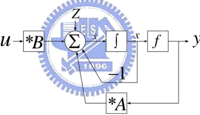
As shown in Fig. 1, the state equation of CNN can be represented by

( )

( )

( )

( )

∑

∑

( )

(

( )

)

(

( )

( )

)

where i, j refers to a grid point associated with a cell on the 2-D grid, and

k, l

∈

cell i, j. A and B are the nonlinear cloning templates [10].The feature of the Eq. (2-2) has been plotted at Fig. 2.

In many applications, the templates A and B and the threshold I are translation invariant. In the case of single variable A and B functions, the linear (space-invariant) template is represented by the following additive

( )

( )

∑

∑

When the template is space invariant each cell is described by a simple identical cloning template defined by two (2r + 1) × (2r + 1) real matrices A and B, as well as the constant term I. In addition, as a very special case, if the input and the initial state values are sufficiently small and f is piecewise linear, then the dynamics of the CNN array is linear. Unlike other standard analog processing arrays, or neural networks, the one-to-one geometric (topographic) correspondence between the pro- cessing elements and the processed signal-array elements ( e.g., pixels) is of crucial importance. Moreover, the template has geometrical meanings which can be exploited to provide with geometric insights and simpler design methods.

Σ

∫

f

1

−

*A

*B

Z

u

y

Fig. 1: The dynamic route of state in CNN.

( ) x t ( ) y t 1 1 -1 -1

2.2 Physical Implementation

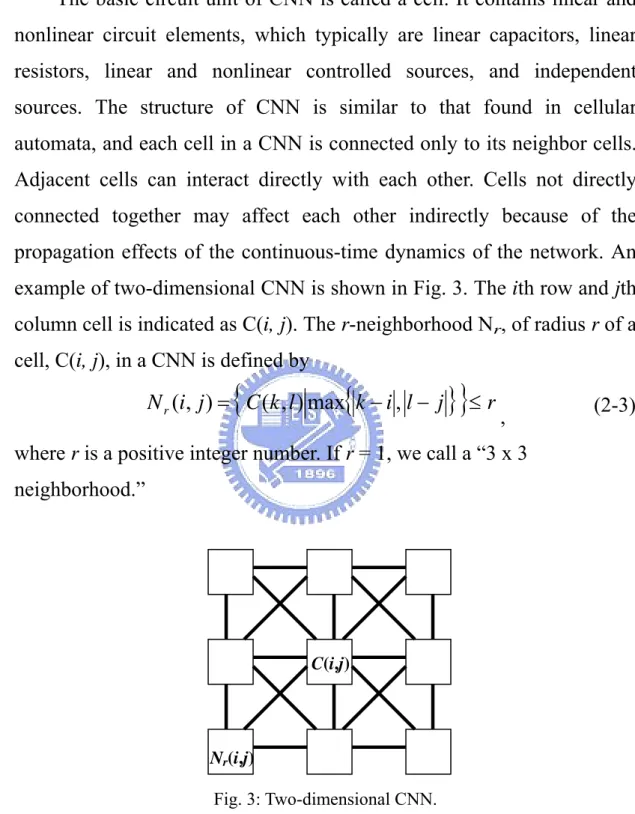
The basic circuit unit of CNN is called a cell. It contains linear and nonlinear circuit elements, which typically are linear capacitors, linear resistors, linear and nonlinear controlled sources, and independent sources. The structure of CNN is similar to that found in cellular automata, and each cell in a CNN is connected only to its neighbor cells. Adjacent cells can interact directly with each other. Cells not directly connected together may affect each other indirectly because of the propagation effects of the continuous-time dynamics of the network. An example of two-dimensional CNN is shown in Fig. 3. The ith row and jth column cell is indicated as C(i, j). The r-neighborhood Nr, of radius r of a

cell, C(i, j), in a CNN is defined by

{

}

{

}

where r is a positive integer number. If r = 1, we call a “3 x 3 neighborhood.”

Fig. 3: Two-dimensional CNN.

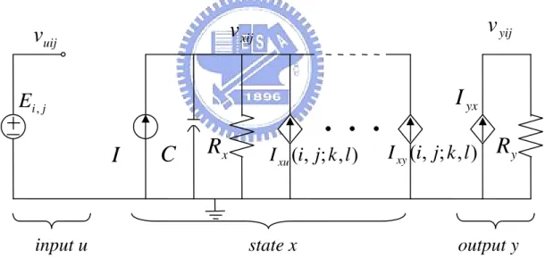
A typical example of a cell C(i, j) is shown in Fig. 4, where the suffixes u, x, and y denote the input, state, and output, respectively. The node voltage Vxij of C(i, j) is defined as the state of the cell whose initial

C(i,j)

condition is assumed to have a magnitude less than or equal to 1. The node voltage Vuij is defined as the input of C(i, j) and is assumed to be a

constant with magnitude less than or equal to 1. The node voltage Vyij is

defined as the output. C is a linear capacitor; Rx, and Ry, are linear

resistors; I is an independent current source; Ixy(i, j; k, I) and Ixu(i, j; k, r)

are linear voltage-controlled current sources with the characteristics Ixy(i,

j; k, l) = A(i, j; k, I) Vykl and Ixu(i, j; k, I) = B(i, j; k, l) Vykl, for all C( k, l)

∈

defined by

(

)

Eij is a time-invariant independent voltage source.

Fig. 4: The circuit of a CNN cell.

Applying KCL and KVL, the circuit state equation of a cell is easily derived as follows: State equation: . 1 ; 1 , ) ( ) , ; , ( ) ( ) , ; , ( ) ( 1 ) ( ) , ( ) , ( ) , ( ) , ( N j M i I t v l k j i B t v l k j i A t v R dt t dv C j i N l k C ukl j i N l k C ykl xij x xij r r ≤ ≤ ≤ ≤ + + + − =

∑

∑

E

I

C

R

I

(

i

,

j

;

k

,

l

)

I

R

v

v

v

Output equation: . 1 ; 1 |), 1 ) ( | | 1 ) ( (| 2 1 ) ( N j M i t v t v t

vyij xij xij

≤ ≤ ≤ ≤ − − + − = _(2-6) Input equation: . 1 ; 1 , ) ( N j M i E t v_{uij ij} ≤ ≤ ≤ ≤ = (2-7) Constraint conditions: , 1 | ) 0 ( |vxij ≤ 1≤i≤M;1≤ j ≤N. (2-8) , 1 | ) 0 ( |v_uij ≤ 1≤i≤M;1≤ j ≤N. (2-9) Parameter assumptions: ), , ; , ( ) , ; , (i j k l A k l i j A = 1≤i,j≤M;1≤i,j≤ N. (2-10) 0 , 0 > > R_x C (2-11)

Chapter 3

Biological-Inspired Model for

Hybrid-Order Texture Boundary

Detection during Early Vision

The physiological and psychophysical findings in the preceding section do not lead to a convenient computational model for the hypothesized cortical channels. In this chapter, a new boundary detection algorithm is proposed. This algorithm combines the first-order and second-order features to model pre-attentive stage of human visual system. A simple hybrid-order channel model is described in the following.

3.1 Whole Architecture

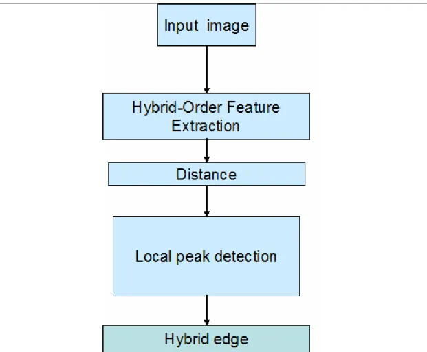
Fig. 5 shows a simplified flow-chart of the proposed algorithm. We first extract first-order by Gaussian low-pass filter and second-order features by Gabor filters respectively. After feature extraction, every pixel of the output is an N+1 dimensional vector for (N Gabor filters and 1 Gaussian filter), and then we measure the difference of each pixel with its neighbor. Because pixels belong to the same region have similar feature, the difference between them should be small. Then we keep the value which is bigger than a threshold and make pixels of which value are smaller than threshold to zero. We would get coarse boundaries which have Gaussian-like distributions.

With boundaries which have Gaussian-like distribution, we may go a step further to thin these boundaries by local peak detection, and after this stage we will get boundaries similar to human visual system.

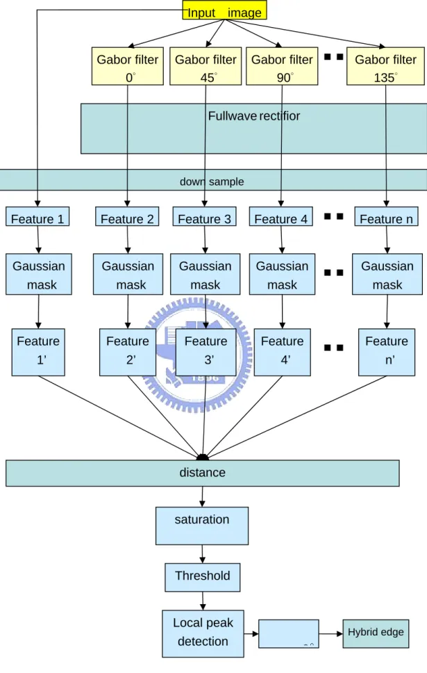
The proposed hybrid-boundary detection algorithm will be presented in detail, and the simplified block diagram is shown in Fig. 5, and Fig. 6 is a detailed version of Fig. 5.

Fig. 6: detailed block diagram for hybrid-order boundary detection algorithm Fullwaverectifior down sample Gabor filter 90° Feature 4 Feature 4’ Gaussian mask distance Threshold Input image saturation Hybrid edge Feature 1 Feature 1’ Gaussian mask Gabor filter 45° Feature 3 Feature 3’ Gaussian mask Gabor filter 0° Feature 2 Feature 2’ Gaussian mask Gabor filter 135° Feature n Feature n’ Gaussian mask Local peak detection

0°

3.2 Hybrid-Order Feature Extraction

3.2.1 First-Order Feature Extraction

DoG (difference of Gaussian) function can be used in detecting boundaries. Two Gaussian filters with different values of σ are applied in parallel to the image. Then the difference of the two smoothed instances is computed. It can be shown that the DoG operator approximates the LoG (Laplacian of Gaussian) one which has been widely used in boundary detection.

We can think of the receptive field shape of a retinal ganglion cell as the linear spatial weighting function of the cell. That is, we can model the retinal ganglion cell as a linear neuron, where the receptive field tells us what the weights are. Using the function R( yx, ) to characterize the receptive field shape using the DoG model, we compute the output of a model retinal ganglion cell as

∑

where I( yx, )_{is the input image.}

The operation of DoG function can be divided into two stages, Gaussian convolution and gradient. Gaussian convolution is somehow like extracting the mean of local region which is we called first-order feature here, and gradient is measure the variation of first-order feature.

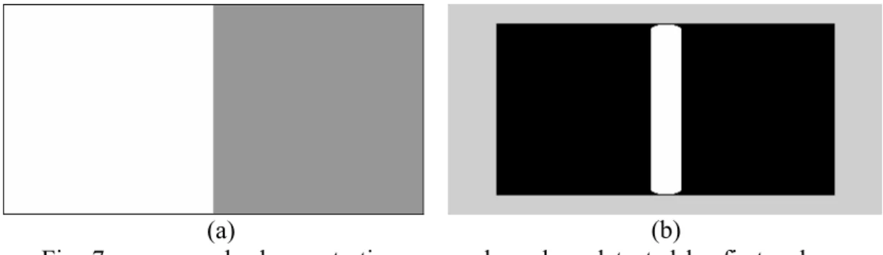
Fig. 7 illustrates the coarse boundary between two patterns with pure first-order features, and it is detected by only using first order feature.

(a) (b)

Fig. 7: an example demonstrating coarse boundary detected by first-order feature (a) input image; (b) boundaries detected

3.2.2 Second-Order Feature Extraction

3.2.2.1 Gabor Function

Gabor function consists of a Gaussian function modulated by a sinusoidal function, and it can be described as following:

(

)

[

]

π

( )

(

)

( )

( )

(

)

λ = / _{is the aspect ratio,} σ_{x is the STD of Gaussian in x axis,} σy

is the STD of Gaussian in y axis, and σ =σx =λ⋅σy.

An important property of Gabor filters is that they have optimal joint localization, or resolution, in both the spatial and the spatial-frequency domains. By signal processing we know that a Fourier transform of Gaussian function is still Gaussian function, and by “uncertainty principle” we know that Gaussian function is the only function that can reach the optimal constraint of uncertainty principle. Uncertainty principle describes the optimal resolution in both the spatial and the spatial-frequency domains.

proved that this action only cause movement in frequency domain, and it wouldn’t affect the resolution of Gaussian function in spatial and the spatial-frequency domain. It means that Gabor function inherit property of Gaussian possessing optimal resolution in both domain, and this property is why Gabor filter is suitable for texture segregation.

3.2.2.2 Full-Wave Rectifier

Like other filter-rectifier-filter model, rectifier operation is taken after convolution by Gabor filters. It has been generally acknowledged that V1 cells have a property like half wave rectifier property, and the intervening rectifier ensures that the fine-grain positive and negative portions of the carrier do not cancel one another when smoothed by the later filter. The rectifier operation also breaks the identical equality between linear filter theory and Fourier transformation.

3.2.2.3 Gaussian Post Filter

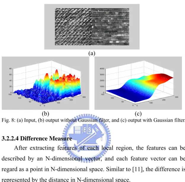
After being stimulated by bars with specific orientations, the output of V1 cells responding to similar orientation will aggregate together. The region with the same property will respond stronger than regions which consist of elements with different properties, and it is consistent with the “localization” property of texture. We can simulate this effect by a Gaussian post filters, it is somewhat like averaging with different weighting which is inverse proportion to distance to the center of the post filter. In the field of texture segmentation, Gaussian smoothing is an important procedure to eliminate features that varying abruptly.

Fig. 8 (b) shows the result after rectifier without Gaussian filter, and Fig. 8 (c) is the result of Fig. 8 (b) after Gaussian filter. In Fig. 8 (c) there is a ramp-like feature profile, and the next step is to detect the position

where the variation of difference is maximum.

(a)

(b) (c)

Fig. 8: (a) Input, (b) output without Gaussian filter, and (c) output with Gaussian filter.

3.2.2.4 Difference Measure

After extracting features of each local region, the features can be described by an N-dimensional vector, and each feature vector can be regard as a point in N-dimensional space. Similar to [11], the difference is represented by the distance in N-dimensional space.

3.2.2.5 Gabor Filter Bank

Besides orientation selectivity, Gabor filters also have frequency selectivity with different parameter. With these two properties, Daugman extended the original Gabor filter to a 2D representation [12]. There have been many researches about Gabor filter bank. Jain and Farrokhnia [13] suggested a bank of Gabor filters, i.e., Gaussian shaped band-pass filters, with dyadic coverage of the radial spatial frequency range and multiple orientations.

by CNN, the structure can’t be too complex. In this thesis we use totally sixteen Gabor filters to extract 2nd-order feature to do our experiments. All these Gabor filters have the same Gaussian shape in frequency and scatter uniformly in four orientations and four frequency bands.

3.3 Saturation and Local Maximum Detection

3.3.1 Saturation

In this thesis we choose the mean of difference of total pixels as threshold, and the situation occur most frequently is that some boundaries with relative lower magnitude is eliminated. This is because of a relative huge region being considered to measure local feature, and the scale of difference between different patterns vary enormously. Obvious boundaries and cause relatively great difference and raise the mean of difference, and the boundaries which are not so obvious causing relative low difference will be eliminate.

We use natural log transformation to simulate the saturation effect to alleviate this problem. It can suppress strong responses which may affect the mean (threshold) to much, but still keep the position of maximum difference where we assume boundaries lying.

3.3.2 Local Maximum Detection

The coarse boundaries detected after taking threshold are too thick, and local maximum detection is used to thin it, but it’s difficult to be implemented on CNN-based algorithm. Local maximum detection is assumed that the difference between different patterns should be maximal at their boundary, and the boundary will be right there.

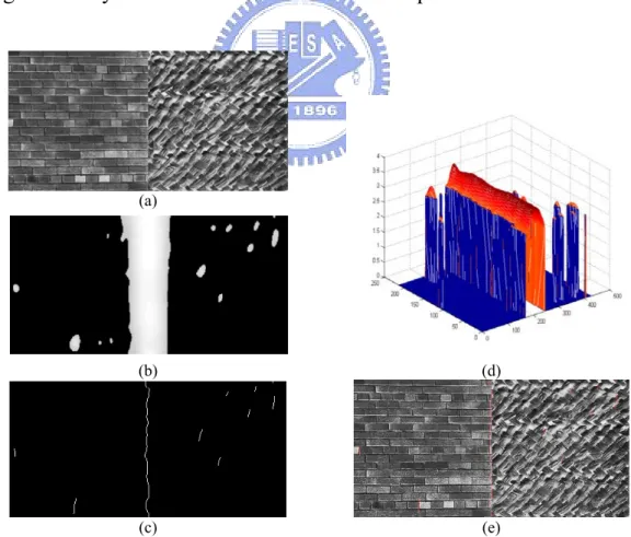
column by column to find local maximums in x and y axes. (2) Sort the peaks we find in 1) in descending order. (3) Keep points with higher order in each line and column, and the output is binary. The values at that pixel regarded as boundaries (points with higher order) are 255, and others are 0. The number of peak-points we keep in (3) is depending on the complexity of input image, and in our testing images we use two.

Fig. 9 is an example demonstrates the peak detection in the algorithm. Fig. 9 (a) is an input image, and Fig. 9 (b) is the detected coarse boundary. Fig. 9 (c) is the 3D version of Fig. 9 (b), and in this figure the vertical axis is intensity. Fig. 9 (d) is the result of Fig. 9 (c) by taking peak detection. Fig. 9 (e) is the superposition of Fig. 9 (a) and Fig. 9 (c). From Fig. 9 (e) we can observe that the detected boundaries have high accuracy which is consistent to our assumption.

(a)

(b) (d)

(c) (e)

Fig. 9: (a)input (b)coarse boundary (c)3D version of (b) (d)(c)after peak detection (d)superposition of (a) and (d)

3.4 Down Sampling and Up Sampling

After rectifying second-order features of different orientations have been extracted, and the output of each channel has the same size to input images (each texture pattern has 640×640 pixels). The amount of features is proportional to the number of channels. With the number of channels increasing, it cause heavy computational loading in following processing, and we improve this problem by down sampling feature space (in our experiments we down sample by 3).

By choosing appropriate down sampling rates we can accelerate the following processes without losing too much accuracy. After boundaries have been detected, we will up sample before output. It will map detected boundaries to the corresponding position in original input.

This mechanism is similar to human vision, and trade-off of spatial accuracy and computational loading is a common problem in human vision system and the proposed algorithm. In fact the whole visual pathway is like serial processes of information extraction and data compression.

Without attention, human vision generally has low resolution in the field of vision, and even with attention we only have high resolution in a relatively tiny proportion of the field of vision. Although in this thesis we only consider the Pre-attentive situation, we still have acceptable spatial-accuracy for boundary detection which can be observed after local peak detection.

Chapter 4

CNN-Based Texture Boundary

Detection

In this chapter, the CNN-based texture boundary detection (TBD) in is described. The whole architecture of original algorithm cannot be implemented completely, and we have to modify the original algorithm to a new algorithm called modified TBD. Modified TBD removes the local maximum detection, slightly modifies the threshold processing, and remain the other blocks of the original algorithm. Therefore, the results of the modified TBD will be thick boundaries instead of the thin boundaries, but still clear and exact boundaries.

The architecture of the modified TBD still contains many blocks, which include Gabor filter, rectifier processing, Gaussian filter, distance, and threshold processing. In order to reduce the complex computation, the modified TBD can be reformulated naturally as well-defined tasks called CNN where the signal values are placed on a regular geometric 2-D grid, and the direct interactions between signal values are limited within a finite local neighborhood. Recall Eq. (2-1), and template A and B, and threshold I are designed to implement each block in the modified TBD with the MatCNN simulator. For another important purpose, analog circuit implementation, we run the CNN algorithm to the stable situation to correspond to the simulation on Hspice [14].

4.1 CNN-Based Gabor Filtering and Gabor Filter

Bank Set

In modified TBD algorithm, the Gabor filter plays an important role in the second-order feature extraction. In image processing, filter means that image does convolution with a mask which may be a high pass, band pass, or low pass filter. In CNN, what template B works is the same as the convolution in image processing and we can easily implement convolution by setting template A = 0, template B = the value of the convolution mask and threshold I = 0. On the other hand, any convolution processing can be implemented by assigning the same value and the same resolution to template B.

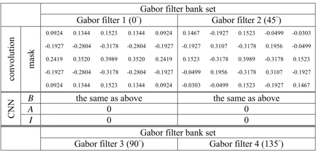
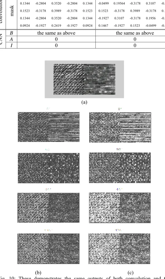
Gabor filter bank set in the thesis contains four Gabor filters and to implement one Gabor filter needs one CNN array such that there are four CNN arrays in Gabor filter bank set. Table 1 shows that there are four Gabor filters with different orientations of the Gabor bank set and lists both mask values and CNN parameters. As shown in Fig. 10, the results of four Gabor filters which implemented by convolution processing and CNN array processing are the same.

Table 1 : Gabor filter bank set ( four Gabor filters ). Gabor filter bank set

Gabor filter 1 (0°) Gabor filter 2 (45°)

0.0924 0.1344 0.1523 0.1344 0.0924 0.1467 -0.1927 0.1523 -0.0499 -0.0303 -0.1927 -0.2804 -0.3178 -0.2804 -0.1927 -0.1927 0.3107 -0.3178 0.1956 -0.0499 0.2419 0.3520 0.3989 0.3520 0.2419 0.1523 -0.3178 0.3989 -0.3178 0.1523 -0.1927 -0.2804 -0.3178 -0.2804 -0.1927 -0.0499 0.1956 -0.3178 0.3107 -0.1927 convolution mask 0.0924 0.1344 0.1523 0.1344 0.0924 -0.0303 -0.0499 0.1523 -0.1927 0.1467

B the same as above the same as above

A 0 0

CNN _{I 0 0}

0.0924 -0.1927 0.2419 -0.1927 0.0924 -0.0303 -0.0499 0.1523 -0.1927 0.1467 0.1344 -0.2804 0.3520 -0.2804 0.1344 -0.0499 0.19564 -0.3178 0.3107 -0.1927 0.1523 -0.3178 0.3989 -0.3178 0.1523 0.1523 -0.3178 0.3989 -0.3178 0.1523 0.1344 -0.2804 0.3520 -0.2804 0.1344 -0.1927 0.3107 -0.3178 0.1956 -0.0499 convolution mask 0.0924 -0.1927 0.2419 -0.1927 0.0924 0.1467 -0.1927 0.1523 -0.0499 -0.0303

B the same as above the same as above

A 0 0

CNN

I 0 0

Fig. 10: These demonstrates the same outputs of both convolution and CNN processing.(a)input; (b)outputs of Gabor filters; (c)outputs of rectifier processing.

(a)

4.2 CNN-Based Rectifier Algorithm

Rectifier operation is taken after convolution processing by Gabor filters. It has been generally acknowledged that has a property like half- wave rectification property, and the rectifier equation we proposed in this thesis is the simplest mode, f x y( , ) | ( , ) |= f x y .

The simplest rectifier equation is the same as the absolute-value operation which is a very easy equation in Matlab coding. In order to implement rectifier processing by using CNN array, we have to design CNN parameters, template A, B and threshold I.

CNN-based rectifier processing has three steps : Step 1 (positive) :

By setting the following parameters, we can shift the image down to cut off the negative part of image and retain the positive part.

A = [0]; B = [1]; I= -1; INPUT = input; output1 = OUTPUT

And then by setting the following parameters, we can shift the image back to the original value without negative part.

A = [0]; B = [1]; I= 1; INPUT = output1; output2 = OUTPUT

Step 2 (negative) :

It’s very similar to step 1, but inversing the image has to be done first and this is what template B = -1 does.

A = [0]; B = [-1]; I= -1; INPUT = input; output3 = OUTPUT

And then shift the image back with only positive part. The positive part is the inversing image of original image with only negative part.

A = [0]; B = [1]; I= 1; INPUT = output3; output4 = OUTPUT

Step3 (addition) :

Final step is to add positive and negative part together. output of rectifier processing = output2 + output4

By following the three steps, we can get the output image after rectifier processing. As shown in Fig. 10, the results of four rectifier processing after Gabor filters which implemented by absolute-value processing and CNN array processing are the same. Specially noticed, the step 3 can be easily implemented by the simple operation, addition, because of CNN array of the current-mode analog circuit.

4.3 CNN-Based Gaussian Filter

4.3.1 Range of Image

Generally speaking, most image processing ignores the range of the image value and at last normalize the final image output to the correct range. The algorithm described in Chapter 3 is the same, but CNN-based algorithm has its own property that is the dynamic range which will affect the image processing before normalizing and make the values of some pixels to become saturation. The effect will lose some or even more important information of image. Therefore, we have to define a range of our image processing. All image processing in this thesis is based on gray-scale and the gray-scale is 256 levels.

The CNN-Based Gaussian filter processing is the most possible to make the image out of the range to saturation, so we discuss this problem of range here. In this thesis, we can guarantee that if the image value of CNN-Based Gaussian filter processing is on the correct range, then the image value of other processing will be sure to on the correct range.

The output range of CNN is from -1 to 1 as shown in Fig. 2 and what we have to choose the range of image value is from zero to 1 because the range from -1 to zero will be used difficultly and indirectly. After choosing the range of image value, we have to ensure that the

image range of every processing will on the correct range. In this thesis, we are sure that the image value in on the correct range unless the use of saturation processing.

4.3.2 CNN-Based Convolution

In this section, we will show that large size convolution mask, like 51 by 51, can be implemented by much smaller size, only 5 by 5 template

A and B of CNN array. But the procedure is too complex; we will discuss

an easier method first.

The easier method to do CNN-based convolution is like the method shown in Section 4.2 and the method is to use only template B and set the same value as the mask. But the method has a very big problem that is problem of size meaning that the size of template B will be the same as the convolution mask. Based on the method, the CNN-based Gaussian- like filter will be implemented by using 51 by 51 template B. How large the size of template B is and it is impossible to implement on either CNN-based algorithm or analog circuit. We cannot choose this method and what we use is only 5 by 5 template A and B of CNN array.

Before proving the method of using only 5 by 5 template A and B of CNN array to implement convolution, to briefly introduce the convo- lution is necessary. If the input is the impulse sequence (only one pixel has value), the resulting output is called the impulse response of the filter. The input and output of a linear space-invariant (LSI) filter may be easily related via the impulse response of the filter as follows : Any input (image) can be thought of as the sum of an infinite number of shifted and weighted impulse sequences, and by space-invariance and by linearity, the output is thus

( , )

( , )

(

,

)

s a t b

g x y

w s t

f x

s y

t

=− =−

=

∑ ∑

⋅

+

+

where a = (m-1)/2 , b = (n-1)/2 and size of the filter mask is m by n.

Therefore, we have to show the space-invariance and linear property of the CNN-based convolution processing. The ideal space-invariance property is shown in Fig. 11 and if the waveform shown in Fig. 11 (a) is the impulse response of an impulse sequence, the impulse response of the shifted impulse sequence will be shown in Fig. 11 (b). The ideal linearity property is shown in Fig. 12 and if the waveform shown in Fig. 12 (a) is the impulse response of an impulse sequence, the impulse response of the weighted impulse sequence will be shown in Fig. 12 (b) and if adding two impulse responses is shown in Fig. 12 (c), the ideal output will be shown in Fig. 12 (d).

Fig. 11: The ideal space-invariance property. (a) The impulse response. (b) The shifted impulse response.

Fig. 12: The ideal linearity property. (a) The impulse response. (b) The weighted impulse response. (c) Two impulse responses before adding. (d) The response of adding both shifted and weighted impulse sequences.

(a) (b)

(a) (b)

Fig. 13 shows the space-invariance and linear property on CNN- based convolution processing. Fig. 13 (a) and (b) show the space- invariance property and we are sure that the waveform in (b) equals to the shifted waveform in (a). Fig. 13 (b), (c) and (d) show the linearity property and we are sure that the waveform in (d) equals to the output after adding waveforms in (b) and (c). Especially noted that the parameters of CNN array are 5 by 5 template A and 3 by 3 template B, and the size of impulse response is large than size of templates.

(a) (b)

(c) (d)

Fig. 13: The properties of CNN-based convolution processing. (a) The impulse response. (b) The shifted impulse response. (c) The weighted impulse response. (d) The response of adding both shifted and weighted impulse sequences.

4.3.3 Gaussian Filter

Everyone knows that the Gaussian function has its own properties and the Eq. (3-3) shows the Gaussian function equation. To discuss the properties is not necessary here and what we have to discuss is how the CNN-based Gaussian filter is similar to the real Gaussian filter. As the properties discussed in Section 4.4.2, if the impulse response of the CNN-based Gaussian filter is similar to the 2-D real Gaussian functions shown in Fig. 14 (a), then the CNN-based Gaussian filter has the same function as the convolution processing of real Gaussian filter. Fig. 14 (a) shows two Gaussian functions with different parameters, and relation between the two Gaussian functions is something like zoom in or zoom out on the x-axis.

We have tried many methods and many kinds of parameters of CNN, and we got some important experience. Fig. 14 (b) and (c) show the 3-D and 2-D impulse responses of CNN-based Gaussian filter using only template A and the results are very similar to real ones, but using only template A has a risk of losing information that is because of the properties of template A on analog circuit implementation. Therefore, we have to use both template A and B to have a fixed input to avoid losing information. Fig. 14 (d) and (e) show the 3-D and 2-D impulse responses of CNN-based Gaussian filter using template A (5 by 5 Gaussian function) and B and the results are not very good but good enough to be used. These errors can not be avoided because the template B of size 5 by 5 has finite number of fixed inputs and template A must have a large deno- minator which approximately equals to the summation of all numerators of template A.

Therefore, the design of the CNN-based Gaussian filter in this thesis is to design template A and B, as following,

12 13 15 13 12 13 17 18 17 13 0 1 0 15 18 20 18 15 1 1 1 , I =0. 13 17 18 17 13 0 1 0 A = 1 Kai 12 13 15 13 12 , B = 1 Kbi

If Ka is bigger than 372 (the summation of all numerators of template

A), the impulse response of CNN-based Gaussian filter becomes thinner

than Fig. 14 (d). If Ka is smaller than 372, the impulse response

becomes fatter and if Ka is smaller enough, the impulse response will

goes to saturation. If Kb is too big, the impulse response will also goes

to saturation because the Kb control the amplitude of the impulse

response. If saturation happens, the impulse response is not one of CNN-based Gaussian filter any more.

(d) (e)

Fig. 14: The impulse responses of the CNN-based Gaussian filter. (a) The real 2-D Gaussian functions with different σ . The 3-D impulse response in (b) and the 2-D impulse response in (c) of the CNN-based Gaussian filter with only template A. The 3-D impulse response in (d) and the 2-D impulse response in (e) of the CNN-based Gaussian filter with template A and B.

4.4 CNN-Based Distance and Threshold Algorithm

4.4.1 Distance Processing

After extracting features of each local region, the feature can be described by a N-dimensional vector, and each feature vector can be regard as a point in N-dimensional space. In this thesis, we only compute the difference between features of each pixel to pixels right behind and below to it and then use threshold to cut off useless pixels to remain the texture boundary.

CNN-based difference between features of each pixel can be easily implemented by setting the parameters of CNN array as following,

0 0 0

A = 0 , B = 0 1 -1 , I =0,

0 0 0

arrays. After this, the design is to do much easier processing, rectifier processing instead of complex computations which are square processing and square root processing, and sum the five distance value arrays pixel by pixel to a new image array. Rectifier processing mentioned in Section 4.3 has similar function but is not so powerful to enhance the distance.

4.4.2 Threshold Processing

CNN-based threshold processing is based on original threshold processing, but has a little difference as shown in Fig. 15. The CNN-based threshold processing will pull down the value as shown in Fig. 15 (b). The original value which is larger than Ith will subtract Ith,

and the original value which is smaller then Ith will be pulled down to

zero.

The first step of CNN-based threshold processing is set the following parameters, and we can shift the image down to cut off what we don’t want of image and retain what we want.

A = [0]; B = [1]; I= -(1+Ith); INPUT = input; output1 = OUTPUT

And then by setting the following parameters, we can shift up the minimum value of image to zero.

A = [0]; B = [1]; I= 1; INPUT = output1; output2 = OUTPUT

Finally, the difference between two threshold processing is not a large effect because we can enhance the image and the images will be very similar to each other.

The modified TBD is somewhat different from the original TBD. We modify the threshold processing and ignore the local maximum detection after threshold processing of original algorithm proposed in Chapter 3 because these functions are difficult to be implemented by the current-mode CNN circuit.

Fig. 15: The relation of image value changing between before and after threshold processing on (a) original algorithm and (b) CNN-based algorithm.

Ith Ith

before threshold processing

after after

before threshold processing Slope = 1 Slope = 1

Chapter 5

Design of Application-Driven CNN

Circuits

We shall implement CNN-based TBD algorithm proposed in Chapter 4 with analog current-mode circuits and simulate the designed circuit with HSPICE.

5.1 Architecture of CNN-Based Texture Boundary

Detection

According to the proposed algorithm and based on the processing element in Fig. 18, the system architecture of the analog circuit for the CNN-based TBD is constructed here. The circuit system is a conceptual block diagram of an analog computer shown in Fig. 16. It consists of the 16×16 CNN array with templates, the analog absolute value circuit, and the summation unit. To reduce design complexity and die size for sophisticated process technology in our experiment, a programmable current-mode CNN array is designed, and every current-mode CNN array shown in Fig. 16 can be replace by the programmable current-mode CNN array with different template A, B and threshold I. Of course, the CNN size can be increases in real production depending on the tradeoff between required real-time rate and cost for various applications.

The activity of the system is divided into four main function, Gabor filter, Gaussian filter, distance, and threshold, as described in Fig. 16. At

first, a digital image is transferred by DAC function to currents and fed into the network as input values in CNN array. These currents are defined positive and assigned to the positive part of the CNN sigmoid function. The network then performs the Gabor filters with four orientations (four kinds of template A). Here we will obtain the results with both positive and negative values in the steady state and the results are fed into the analog absolute value circuits. After that, the results become all positive values and fed into Gaussian filters with the same templates. The results of the Gaussian filters are all positive values and then fed into distance units with the same templates. We will feed results of distance units into analog absolute value circuits one more, and get positive results. The network then performs the summation units implemented by connecting results of five absolute value units pixel by pixel to new results of a new array (because of current-mode). Finally, the network feeds the results of summation units and a threshold value Ith which is the mean of these

results to threshold units with the same templates.

To realize the whole analog circuit efficiently, we modify the Eq. (2-1) to a new current-mode equation as following,

( )

( )

( )

( )

, ( , ) , ( , )

xij xij i j k l ykl i j k l ukl i j k l Nr i j k l Nr i j

i t i t A i t B i t I

∈ ∈

= − +

∑

∑

and design a single current-mode CNN neural cell in Fig. 17 which shows the schematic view of the modified single neural element (cell). The input current to the cell can be set continuously within the range limited by the unit current. This will result in the nonlinear function for iyij (t) shown in

Fig. 17. The sigmoid function is realized by using two-level shifted current mirrors connected in series. The saturation levels of the sigmoid with slope set as 1 are determined by the current source IL. This piecewise

approximation of symmetric current limiting with cascaded current mirrors has been used effectively in other implementations [6], but most

of implementations are applied for binary image processing only.

In addition, a single cell includes the neuron cell unit, the template A unit, and the template B unit shown in Fig. 17. The neural cell unit for the proposed algorithm must contain two input nodes. To obtain negative template coefficients in the current-mode design, both the template A and

B units contain one current inverter in our design and the details will be

described in following section. The correct cell activities are regulated by the switches within the single cell circuit, whose functionalities are listed in Table 2.

Table 2 : Functionalities of the switches in the schematic circuit in Fig. 17. Logic Switch High Voltage (3.3V) Low Voltage (0V) Vac Normal operation Initial phase

Vtap Choosing positive template A Choosing negative template A Vtbp Choosing positive template B Choosing negative template B

Fig. 16: The block diagram of the CNN-based TBD. Current-mode CNN array Input image Absolute value Absolute value Absolute value Absolute value Summation Absolute value Absolute value Absolute value Absolute value Absolute value Gabor filter Gaussian filter Output Distance Threshold Ith 0° 45° 90° 135°

5.2 Basic Processing Element (CNN Cell)

To achieve acceptable resolution with standard procedures, a current- mode CMOS realization of CNN has been proposed in [6]-[9], which was adapted from the implementation in [1]. Based on this design, a generic model of one CNN cell with the current-mode architecture is shown in Fig. 18, where xc_{, u}c_{, z}c_{, and y}c _{are the cell state, input, bias and output}

variable in continuous time. Note that this circuit model is identical to the model given by Eq. (2-1). The model consists of the dynamic block, the nonlinear block, and the weighted block. The dynamic block is composed a continuous time integrator loaded with a bias shifted current mirror. The nonlinear block can determine the output transfer function using the current-mirror rate. A current-mode output characteristic is described in [6]. Note that weighted replication is performed at the output current of each cell. In other words, each cell generates a different output, with the specific weights as A and B indicating the template A and B, for each neighbor.

Fig. 18: Architecture of a generic current-mode CNN cell, where xc_{, y}c_{, u}c_,

and zc _{indicate the state, output, input, and bias.}

6µA, and 4µA are shown in Fig. 19. The slope of simulated sigmoid functions is set to 1. Only positive coefficients are achieved due to the positive feedback network. The realization of negative coefficient values is obtained by connecting the current through a current inverter.

(a) (b) Fig. 19: Simulated sigmoid functions (slope=1) with HSPICE. (a) Positive and

(b) negative slopes in different current gains through a current inverter.

5.3 Templates Design

We now introduce the realization of required CNN templates in the current-mode design. Through a transistor ratio, a positive template value can be obtained as shown in Fig. 20 (a). To generate negative template values, a current inverter is cascaded to the transistor ratio as shown in Fig. 20 (b). To add image input with template A unit to become template

B unit, the image input unit as shown in Fig. 20 (c) is needed. The

position of a current source inspires the direction of output current. With these template units, we design a 5x5 large neighborhood CNN array with a neuron cell unit [15]-[17], 24 template A units, and 25 template B units per cell. In addition, the threshold I can be easily implemented by adding a single current source to the input of the neuron cell unit as shown in Fig. 17 and the implementation of initial state is like the threshold I. The

difference is that the initial state turns on just for a whole and can be different from other initial states of different cells.

Fig. 20 (d) shows a programmable current amplifier [18] with changing the Vvalue and Ibias. The architecture of the CNN-based TBD

contains many CNN arrays with different parameters and to replace fixed templates with programmable templates to be a programmable CNN array is necessary.

(a) (b) (c)

(d)

Fig. 20: Template realization in the circuit of CNN-based TBD, where (a) is for positive output, (b) is for current inverter, (c) is for the image input unit, and (d) is for the programmable current amplifier.

5.4 Boundary Selection

The boundary conditions [19] are defined by the border cells which surround the active grid. Any virtual variable in i must be specified via

Mbin

iuij (t)

Ai,j;k,l．iykl (t)

boundary conditions, of which the most commonly used are for 5×5 neighborhood. Excepting 16×16 cells, the central 8×8 cells are the real array of the image, and the others cells are the boundary cells. The boundary conditions in our design are like padding processing, but are the extending of the central 8×8 cells. The width of the boundary cells depends on the size of the Gaussian filters. The real boundary conditions outside the 16×16 cells can be considered as fixed, zero-flux, and dynamic boundary conditions, respectively [20]. However, the reasons why we choose the zero-flue condition as the boundary condition are due to no input in our algorithm and the natural definition ( no cells, no inputs).

Chapter 6

Experimental Results

6.1 CNN-Base Texture Boundary Detection

The parameters of CNN arrays for CNN-based Gaussian filters is described as following,

and the impulse response of these CNN arrays is shown in Fig. 21

Fig. 21: The impulse response of the CNN-based TBD

The impulse response is not exactly a Gaussian function, such that the results of the CNN-based TBD are different from the results of the modified TBD as shown in Fig. 22.

1 9 15 9 1 9 15 18 15 9 0 1 0 15 18 20 18 15 1 1 1 , I =0, 9 15 18 15 9 0 1 0 A = 1 289i 1 9 15 9 1 , B = 1₃ 10 i

(a) (b)

Fig. 22: (a) Results of the modified Gaussian filters. (b) Results of the CNN-based Gaussian filters.

The results in Fig. 22 (a) are similar to Fig. 22 (b) but not exactly the same. Because the differences between (a) and (b) exist, the results of distance processing and threshold processing after modified Gaussian filters and CNN-based Gaussian filters will be much different as shown in Fig. 23. There are more results of different inputs shown in Fig. 24 and Fig. 25.

0°

45°

90°

Fig. 23: This demonstrates the results of both modified and CNN-based TBD.(a)input; (b) and (c) show the results before and after threshold processing of modified TBD. (d) and (e) show the results before and after threshold processing of CNN-based TBD.

Fig. 24: This demonstrates the results of both modified and CNN-based TBD.(a)input 2; (b) and (c) show the results before and after threshold processing of modified TBD.

(a) (b) (d) (c) (e) (a) (b) (d) (c) (e)

TBD.

Fig. 25: This demonstrates the results of both modified and CNN-based TBD.(a)input 3; (b) and (c) show the results before and after threshold processing of modified TBD. (d) and (e) show the results before and after threshold processing of CNN-based TBD.

6.2 Application-Driven CNN Circuit

Based on the analog circuit implementation described in Chapter 5, we design a 16×16 CNN array to simulate the CNN-based TBD on Hspice. This chapter will show the comparisons between simulation results of MatCNN and that of Hspice, but the image size is only 16×16 which is much smaller than image size using in original algorithm. Therefore, new images with texture of 16×16 size is created and then fed into CNN-based TBD both on MatCNN and Hspice, and the parameters of CNN arrays for CNN-based TBD is designed to be the same as the parameters of CNN arrays for CNN circuit.

Because the size of Gaussian filters changes for 16×16 size, the (a)

(b) (d)

parameters of the CNN-based Gaussian filters have to redesign, but the others parameters do not have to change. The parameters of the Gaussian filters for 16×16 size is described as following,

and the impulse response of CNN-based TBD is shown in Fig. 26.

(a) (b)

Fig. 26: 16×16 CNN array. (a) shows the 3-D impulse response and (b) shows the cut-plane of (a).

The impulse response is similar to a Gaussian function, and the results of the CNN-based TBD are shown in Fig. 27. The input in Fig. 27 (a) is 16× 16, and so are Fig. 27 (d) and (e). Because of the boundary cells, the real images after Gaussian filers are 8×8 as shown in Fig. 27 (f). The final result shown in Fig. 27 (c) is also 8×8.

CNN-based Gaussian filter for CNN circuit has to use the template A. Based on the properties of template A, the dark current in CNN circuit has

1 9 15 9 1 9 15 18 15 9 0 1 0 15 18 20 18 15 1 1 1 , I =0, 9 15 18 15 9 0 1 0 A = 1 400i 1 9 15 9 1 , B = 1 20i

decrease the effect. The offset current can be replaced by the threshold I, and the optimal value of threshold I in this case is 0.2 µA.

(a)

(b)

(c) (d) (e) (f)

Fig. 27: This demonstrates the results of CNN-based TBD.(a)input; (b) and (c) show the results before and after threshold processing. (d) shows the results of Gabor filters, and (e) shows results of rectifier processing after (d). (e) shows the results of Gaussian filters

Except the threshold I (0.2µA), the other parameters for CNN circuits are the same. The results of channel one Gabor filter for CNN circuits are shown in Fig. 28, and are very similar to the results for CNN-based TBD as shown in Fig. 27. The results of channel five Gaussian filter for CNN circuits are shown in Fig. 29, and are very similar to the results for CNN-based TBD as shown in Fig. 27. The whole results of Gaussian filters for CNN circuits are shown in Fig. 30, and the results are not as good as shown in Fig. 27, but still clear and correct.

(a) (c)

(b) (d)

Fig. 28: This demonstrates the 16×16 results of channel one Gabor filter for CNN circuits with using the input as shown in Fig. 27 (a). The 3-D result of channel one after Gabor filter is shown in (a), and the cut-plane of (a) is shown in (b). (c) shows the image of (a). (d) shows the result after rectifier processing of (c).

(a) (c)

(b) (d)

Fig. 29: This demonstrates the 16×16 results of channel five Gaussian filter for CNN circuits with using the input as shown in Fig. 27 (a). The 3-D result of channel five after Gaussian filter is shown in (a), and the cut-plane of (a) is shown in (b). (c) shows the image of (a). (d) shows the central 8×8 image of (c).

(b)

(a) (c)

Fig. 30: This demonstrates the 16×16 results of Gaussian filter for CNN circuits with using the input as shown in Fig. 27 (a). The results of five channels after Gaussian filter is shown in (a), the result after distance processing is shown in (b), and the result is shown in (c).

Chapter 7

Conclusions and Future Works

In this thesis, a biological-inspired model for hybrid-order TBD algorithm, which mimics mechanism of early stage of human vision is proposed and experimental results are generally consistent to human visual sensation. Due to the parallel signal processing of Cellular Neural Networks (CNN), the computation time will greatly decrease. Contrary to the original biological-inspired model for hybrid-order TBD algorithm which has local maximum detection, the modified TBD algorithm can completely transfer to CNN-based TBD and be implemented on CNN-based analog circuits. Without local maximum detection, the boundaries of results for the CNN-based TBD are thick, but clear and exact. The CNN-based TBD implements a 51×51 or any size Gaussian filter with different template A and has the potential to extend the size of filters for any function to any size by using the CNN array with only template A and B. The size of the Gabor filters in this thesis is still 5×5 and to extend the size to a more suitable size will more match the frequency of input images. It will be one research of our future works for the CNN-based TBD.

We also designed an effective current-mode CMOS circuit using cascaded current mirrors with fixed or programmable templates to implement the CNN-based TBD. The programmable CNN circuit can implement each function with different templates in the CNN-based TBD. The designed circuits are very suitable for CNN-based image processing in real-time. Simulation results with HSPICE based on the 0.35µm TSMC

2P4M process have demonstrated the superior functionalities of the designed circuit. In the future, many complex image processing algorithms will be implemented on CNN-based circuits in real-time and we can design an effective controller to integrate each block so that the usage of CNN circuits can be reduced.