Semiclassical quantization for the spherically symmetric systems
under an Aharonov-Bohm magnetic flux
W. F. Kao,*P. G. Luan, and D. H. Lin†
Institute of Physics, Chiao Tung University, Hsin Chu 30043, Taiwan 共Received 1 January 2002; published 17 April 2002兲
The semiclassical quantization rule is derived for a system with a spherically symmetric potential V(r) ⬃r(⫺2⬍⬍⬁) and an Aharonov-Bohm magnetic flux. Numerical results are presented and compared with
known results for models with⫽⫺1,0,2,⬁. It is shown that the results provided by our method are in good agreement with previous results. One expects that the semiclassical quantization rule shown in this paper will provide a good approximation for all principle quantum numbers, including the large principle quantum number nⰇ1. The rule is even derived in the large principal quantum number limit nⰇ1. We also discuss the power parameter dependence of the energy spectra pattern in this paper.
DOI: 10.1103/PhysRevA.65.052108 PACS number共s兲: 03.65.Sq
I. INTRODUCTION
In the past 20 years, the Aharonov-Bohm 共AB兲 effect, a topological nonlocal physical effect at the quantum level, has been of much interest in the studies of cosmic string 关1兴, (2⫹1)-dimensional gravity theories 关2兴, and especially in the context of anyon关3兴, which has shed light on the under-standing of the phenomenon of the fractional quantum Hall effect 关4–7兴, superconductivity 关7,8兴, repulsive Bose gases
关9兴, and so forth. There are only a few models coupled to
different potentials along with an AB magnetic flux that can be solved exactly. For the system with both an AB magnetic flux and a spherically symmetric potential of the form V(r)
⫽r(⫺2⬍⬍⬁), the solvable models known to us in-clude the cases with the parameter⫽⫺1,0,2,⬁ 关10–12,16兴. Here is a constant parameter. Note that when⫽⫺1, it is a system with both an AB magnetic flux and a Coulomb potential (ABC) 关10–12兴. This system describes the relative motion of two charged particles, with one of them carrying electric charge and magnetic flux (⫺q,⫺⌽/Z), while the other one carries (Zq,⌽). Here Z(⫽0) is a nonvanishing real number. This system is of much interest in many differ-ent areas关12兴.
In the past three decades, much progress has been made in the semiclassical methods toward the understanding of these systems. These kinds of semiclassical methods provide us with a powerful approximation tool in different areas in or-der to extract useful information from various unsolved problems including the quantization of the classical chaotic systems 关13兴, deformed atomic nuclei, asymmetric fission nuclei关14兴, semiclassical quantum dots, and weak localiza-tion in mesoscopic systems关15兴. In this paper, we will con-sider a generalized system with both an AB magnetic flux and a spherically symmetric potential of the form mentioned above. The set of the parameters (,) will be discussed in the following ranges 共i兲 (⬍0, ⫺2⬍⬍0) and 共ii兲 (
⬎0,⬎0). We will derive a semiclassical quantization rule
of the approximated energy spectra for this set of parameters. The distribution tendency of the energy spectra on different values of the parameter will also be given. By comparing with the known results, including the models with ⫽
⫺1,0,2, we find that our method agrees with these exact
results. In addition, for the exactly solvable model with
⫽⬁, the difference between the exact and semiclassical
re-sults will be shown to be very small from a numerical com-putation. Therefore, we are confident in that our formulas will also provide a good approximation for the two ranges of parameters mentioned above where ⫽⫺1,0,2,⬁.
This paper is organized as follows. In Sec. II, we will derive the semiclassical quantization rule of the AB effect under a spherically symmetric potential. In particular, we will first derive the nonintegrable phase factor of the Green’s function due to the AB effect in a spherically symmetric system. The corresponding radial Schro¨dinger equation will also be derived accordingly. The semiclassical wave func-tions will also be derived according to the semiclassical con-sideration of the Bohr’s corresponding principle. Conse-quently, the quantization rule can thus be obtained by comparing with the well-known WKB phase. We will also study the distribution dependence of energy spectra in vari-ous models in Sec. III. The effect of magnetic flux will also be discussed and emphasized in this section. Finally, in Sec. IV, some conclusions will be drawn. In order to provide a self-contained information, we will show the WKB matching condition of the semiclassical wave functions in the Appen-dix.
II. SEMICLASSICAL QUANTIZATION RULE OF THE AB EFFECT WITH A SPHERICALLY SYMMETRIC
POTENTIAL
The fixed-energy Green’s function G0(r,r
⬘
;E) for a charged particle with mass m propagating from r to r⬘
satis-fies the Schro¨dinger equation冋
E⫺H0冉
r,ប
i “
冊册
G0共r,r
⬘
;E兲⫽␦3共rÀr⬘
兲, 共1兲 *Electronic address: [email protected]where the system Hamiltonian is given by H0⫽⫺ប2ⵜ2/2m
⫹V(r) as usual. In the spherically symmetric cases, the
an-gular decomposition of the Green’s function can be written as G0共r,r
⬘
;E兲⫽兺
l⫽0 ⬁兺
k⫽⫺l l Gl0共r,r⬘
;E兲Ylk共,兲Ylk*共⬘
,⬘兲, 共2兲with Ylkthe well-known spherical harmonics. As a result, the
left- hand side of the Eq.共1兲 can be brought to the following form:
再
E⫺兺
l⫽0 ⬁兺
k⫽⫺l l冋
⫺ ប 2 2m冉
d2 dr2⫹ 2 r d dr冊
⫹ l共l⫹1兲ប2 2mr2册
⫺V共r兲冎
⫻Gl 0共r,r⬘
;E兲Ylk共,兲Ylk*共⬘
,⬘兲. 共3兲For a charged particle in a magnetic field, the Green’s func-tion G is related to G0 by the following equation:
G共r,r
⬘
;E兲⫽G0共r,r⬘
;E兲exp冋
ieបc
冕
r⬘ rA共r˜兲•dr˜
册
, 共4兲 with a globally path-dependent nonintegrable phase factor关17,18兴 given above. Here we have used the vector potential
A(r˜… to represent the magnetic field. For the
Aharonov-Bohm magnetic flux under consideration, the vector potential can be written as A„x…Ä
再
1 2Beˆ 共⬍⑀兲 1 2B ⑀2 eˆ⫽ ⌽ 2eˆ 共⬎⑀兲, 共5兲where the two-dimensional radial length is defined as 2
⫽x2⫹y2 as usual. Moreover, eˆ
is the unit vector of coor-dinate and⑀ is the radius of region where magnetic field exists. Hence the total magnetic flux is given by ⌽⫽⑀2B. Note that the associated magnetic field lines are confined inside a tube, with radius ⑀, along the z axis. Along the region without magnetic field, the path-dependent noninte-grable phase factor is given by
exp
冋
⫺i0冕
P
d
⬘
˙共⬘
兲册
, 共6兲 where we have used the subscript P to represent the path-dependent nature of phase factor and we have denoted ˙ (⬘
)⫽d/d⬘
. Also, 0⫽⫺2eg/បc is a dimensionless number defined by ⌽⫽4g. The minus sign is a matter of convention. According to the discussion in Ref. 关18兴, only phase factors with closed-loop contour are considered where the description of electromagnetic phenomenon are com-plete. Hence, we haven⫽ 1 2
冕
P
d
⬘
˙共⬘
兲, 共7兲with integer values n corresponding the winding number. The magnetic interaction is therefore purely topological. Therefore the nonintegrable phase factor becomes
e⫺i0(2n). 共8兲
With the help of the equality between the associated Leg-endre polynomial P(z) and the Jacobi function Pn(␣,)(z)
关19,20兴, we find that Plk共cos兲⫽共⫺1兲k⌫共l⫹k⫹1兲 ⌫共l⫹1兲
冉
cos 2sin 2冊
k Pl(k,k)⫺k共cos兲. 共9兲Therefore the angular part of the Green’s function in the expression共3兲 can be turned into the following form:
兺
k⫽⫺l l Ylk共,兲Ylk*共⬘
,⬘
兲 ⫽兺
k⫽⫺l l 2l⫹1 4 ⌫共l⫺k⫹1兲 ⌫共l⫹k⫹1兲 ⫻Pl k共cos兲P lk共cos⬘兲eik(⫺⬘)
⫽
兺
k⫽⫺l l冋
2l⫹1 4 ⌫共l⫺k⫹1兲⌫共l⫹k⫹1兲 ⌫2共l⫹1兲册
⫻冉
cos 2cos ⬘ 2 sin 2sin ⬘
2冊
k ⫻Pl⫺k (k,k)共cos兲P l⫺k (k,k)共cos⬘
兲eik共⫺⬘
兲. 共10兲In order to include the nonintegrable phase factor due to the AB effect, we will change the index l into q related by the definition l⫺k⫽q. As a result one can rewrite the Eq. 共3兲 as
再
E⫺兺
q⫽0 ⬁兺
k⫽⫺⬁ ⬁冋
⫺ ប 2 2m冉
d2 dr2⫹ 2 r d dr冊
⫹共q⫹k兲共q⫹k⫹1兲ប 2 2mr2册
⫺V共r兲冎
Gq⫹k 0 共r,r⬘
;E兲 ⫻冋
2共q⫹k兲⫹14 ⌫共q⫹1兲⌫共q⫹2k⫹1兲 ⌫2共q⫹k⫹1兲册
⫻冉
cos 2cos 0⬘
2 sin 2sin ⬘ 2冊
k ⫻Pq (k,k)共cos兲P q (k,k)共cos⬘兲eik (⫺⬘). 共11兲 In addition, the nonintegrable phase in Eq. 共8兲 can now be included with the help of the Poisson’s summation formula共p. 124, 关21兴兲
兺
k⫽⫺⬁ ⬁ f共k兲⫽冕
⫺⬁ ⬁ dy兺
n⫽⫺⬁ ⬁ e2nyif共y兲. 共12兲再
E⫺兺
q⫽0 ⬁冕
dz兺
k⫽⫺⬁ ⬁冋
⫺ ប 2 2m冉
d2 dr2⫹ 2 r d dr冊
⫹ 共q⫹z兲共q⫹z⫹1兲ប2 2mr2册
⫺V共r兲冎
⫻Gq⫹z共r,r⬘
;E兲冋
2共q⫹z兲⫹1 4 ⌫共q⫹1兲⌫共q⫹2z⫹1兲 ⌫2共q⫹z⫹1兲册
冉
cos 2cos ⬘
2 sin 2sin ⬘ 2冊
z Pq(z,z) ⫻共cos兲Pq (z,z)共cos⬘
兲exp关i共z⫺ 0兲共⫹2k⫺⬘
兲兴, 共13兲where the superscript 0 in Gq0⫹khas been suppressed to reflect the inclusion of the AB effect. The summation over all indices k forces z⫽0 modulo an arbitrary integer number. Therefore, one has
再
E⫺兺
q⫽0 ⬁兺
k⫽⫺⬁ ⬁冋
⫺ ប 2 2m冉
d2 dr2⫹ 2 r d dr冊
⫹ 共q⫹兩k⫹0兩兲共q⫹兩k⫹0兩⫹1兲ប2 2mr2册
⫺V共r兲冎
⫻Gq⫹兩k⫹0兩共r,r⬘
;E兲再
关2共q⫹兩k⫹0兩兲⫹1兴 4 ⌫共q⫹1兲⌫共2兩k⫹0兩⫹q⫹1兲 ⌫2共兩k⫹0兩⫹q⫹1兲冎
e ik(⫺⬘)⫻共cos/2 cos
⬘
/2 sin/2 sin⬘
/2兲兩k⫹0兩Pq
(兩k⫹0兩,兩k⫹0兩)
共cos兲Pq
(兩k⫹0兩,兩k⫹0兩)
共cos
⬘
兲. 共14兲Note that the influence of the AB effect to the radial Green’s function is to replace the integer quantum number l with a fractional quantum number q⫹兩k⫹0兩. Analogously the same procedure can be applied to the delta function ␦3(rÀr
⬘
) in the rhs of the Eq. 共1兲 with the help of the fol-lowing solid angle representation of the␦ function:␦共⍀⫺⍀
⬘
兲⫽兺
l⫽0 ⬁兺
k⫽⫺l l Ylk共,兲Y*lk共⬘
,⬘
兲. 共15兲Therefore, for the set of the fixed quantum numbers (q,k) one can show that the radial Green’s function satisfies
再
E⫺冋
⫺ ប 2 2m冉
d2 dr2⫹ 2 r d dr冊
⫹共q⫹兩k⫹0兩兲共q⫹兩k⫹0兩⫹1兲ប2 2mr2册
⫺V共r兲冎
⫻Gq⫹兩k⫹0兩共r,r⬘
;E兲⫽␦共r⫺r⬘
兲. 共16兲As a result, the corresponding radial wave equation reads
ប2 2m d2 dr2u␥共r兲⫹
冋
E⫺冉
V共r兲⫹ ប2 2m ␥共␥⫹1兲 r2冊
册
u␥共r兲⫽0, 共17兲where we have set ␥⫽q⫹兩k⫹0兩, and u␥(r)⬅rR˜ ␥n (r).
Obviously, R˜ ␥n satisfies the spherical Bessel equation
冋
d2 dr2⫹ 2 r d dr⫹冉
2⫺U共r兲⫺␥共␥⫹1兲 r2冊
册
Rn˜ ␥共r兲⫽0 共18兲with the definitions ⫽
冑
2mE/ប2 and the reduced potential U(r)⫽2mV(r)/ប2. For simplicity, we have written R˜ ␥n (r)instead of R˜ ,q,kn (r) in which each set (n˜ ,q,k) denotes a quantum state. Hence the AB effect reflects itself by the cou-pling to the angular momentum in radial Green’s function, which turns the integer quantum number into a fractional one.
To find the semiclassical quantization rule, let us first con-sider the asymptotic form of the bound-state wave functions of a charged particle moving in a spherically symmetric po-tential of the form V(r)⫽r(⬍0,⫺2⬍⬍0) under an AB magnetic flux for the energy limit E→0. Due to the Bohr corresponding principle, this stands for the semiclassi-cal approximation since there are infinitely densed energy levels near E→0⫺. According to Eq. 共17兲, the asymptotic wave equation reads, in the E→0⫺ limit,
ប2 2m d2 dr2u␥共r兲⫺
冉
r ⫹ ប 2 2m ␥共␥⫹1兲 r2冊
u␥共r兲⫽0. 共19兲 We can also perform the following transformations:⫽r
冉
2m兩兩 ប2冊
1/(⫹2)
, u共r兲⫽W共兲. 共20兲
Consequently, Eq. 共19兲 yields d2W
d2 ⫹
冋
⫺␥共␥⫹1兲
2
册
W⫽0, 共21兲which can be further reduced with the help of the following change of variables:
z⫽ 2
As a result, Eq.共21兲 becomes d2v dz2⫹ 1 z dv dz⫹
冋
1⫺冉
2␥⫹1 ⫹2冊
2 1 z2册
v⫽0. 共23兲 This is exactly the Bessel’s equation of integral order 1⬅(2␥⫹1)/(⫹2). The boundary condition 共BC兲 of the
function u(r) in the Eq.共17兲 is simply u(0)⫽0. Therefore, the corresponding BC of v(z) in the Eq. 共23兲 is v(0)⫽0. The Bessel function of the first kind is known to be the solution of the Bessel’s equation. Therefore, by imposing the BC appropriately, one can show that
v共z兲⫽J
1共z兲 共24兲
is the solution of the Eq.共23兲 with the prescribed boundary condition. Therefore, the solution of the radial wave equation near E→0 becomes
u共r兲⫽W共兲⫽z1/(⫹2)J
1共z兲. 共25兲
From the asymptotic behavior of the Bessel function near r →0, or equivalently→0 and z→0, one can show that
u共r兲⬃z1/(⫹2)z(2␥⫹1)/(⫹2)⬃z(2␥⫹2)/(⫹2)⬃r␥⫹1.
共26兲
On the other hand, from the asymptotic behavior of the Bessel function approaching r→⬁,
J␣共z兲→
冑
2 zcos冉
z⫺ ␣ 2 ⫺ 4冊
, 共27兲 one can show thatu共r兲⬃z1/(⫹2)
冑
2 zcos冉
z⫺1 2⫺ 4冊
⬃⫺/4cos冉
2 ⫹2(⫹2)/2⫺1 2⫺ 4冊
. 共28兲 Note that one can also compute the following integral, near the limit E→0, and show that the following identities hold:冕
0 r冑
2m ប2关E⫺V共r兲兴dr⫽冉
2m兩兩 ប2冊
1/2冕
0 r r/2dr ⫽冉
2m兩兩 ប2冊
1/2 2 ⫹2r(⫹2)/2 ⫽⫹22 (⫹2)/2. 共29兲It follows that, in the limit E→0 and r→⬁,
u共r兲⬃r⫺/4cos
冉
冕
0 r冑
2m ប2 关E⫺V共r兲兴⫺1 2⫺ 4冊
⬃r⫺/4sin冉
冕
0 r冑
2m ប2关E⫺V共r兲兴⫺1 2⫹ 4冊
, 共30兲where V(r)⫽r(⬍0,⫺2⬍⬍0). If we take the integra-tion upper bound r as the classical turning point rc, where
V(rc)⫽E , the phase of u(r) can be shown to be the WKB phase 共see the Appendix for details兲
u共rc兲⬀ sin
冋冉
n⫹3
4
冊
册
. 共31兲 Consequently, from comparing the Eqs. 共30兲 and 共31兲, one can extract the following quantization condition冕
0rc
冑
2m关E⫺V共r兲兴⫽冋
n⫹2␥⫹⫹3 2共⫹2兲册
ប,for n⫽0,1,2,3 . . . . 共32兲 Here n is the radial quantum number. Although Eq. 共30兲 is obtained in the limit E→0, or equivalently in the large quan-tum number where nⰇ1, above result can still be extended to all possible values of n. In fact, the integral in Eq.共32兲 can be written in an analytic form. Indeed, with the help of the following change of variables:
Er
⫽csc2, 共33兲
one can rewrite the above integral as
冕
0 rc冑
2m共E⫺V共r兲兲⫽⫺2 冉
E 冊
1/冑
2m兩E兩冕
0 /2 ⫻cos2共sin兲⫺2/⫺2d. 共34兲 In addition, with the help of the following formula共see, for example, Ref.关23兴, p. 8兲:冕
0 /2 cos2q⫺1z sin2 p⫺1zdz⫽⌫共p兲⌫共q兲 2⌫共p⫹q兲, 共35兲 one has冕
0 rc冑
2m关E⫺V共r兲兴⫽⫺2 冉
E 冊
1/冑
2m兩E兩 ⫻冑
4 ⌫冉
⫺1 ⫺ 1 2冊
⌫冉
1⫺1 冊
. 共36兲E⫽⫺兩兩2/(⫹2)
冉
ប 2 2m冊
/(⫹2) ⫻冋
2兩兩冑
冉
n⫹2共q⫹兩k⫹0兩兲⫹⫹3 2⫹4冊
⫻ ⌫冉
1⫺1 冊
⌫冉
⫺1⫺12冊
册
2/(⫹2) , 共37兲where the ranges of the parameters are ,E⬍0, ⫺2⬍
⬍0, n,q⫽0,1,2, . . . , and ⫺⬁⬍k⬍⬁. For example, with the
potential of the form V(r)⫽⫺e2/r, one has
En,q,k⫽⫺mc2
␣2
2关n⫹q⫹兩k⫹0兩⫹1兴2. 共38兲
Here ␣⫽e2/បc denotes the fine structure constant. This agrees with the exact result given in Ref. 关11兴. We see that the AB effect has changed the splitting of energy levels al-though the electron moves in the absence of the magnetic field. In addition, when the flux is quantized, namely, 4g
⫽(2បc/e)⫻ integer, 兩k⫹0兩 is an integer and hence the spectrum is the same as the energy spectrum of the pure hydrogen atom.
To obtain the semiclassical quantization rule for all posi-tive powers ⬎0 of the potential V(r)⫽r, one can per-form the following change of variable:
⫽r␣, u共r兲⫽v共兲 共39兲
and can show that Eq.共17兲 becomes
d2u dr2⫽␣ 22⫹⫺2/␣d 2v共兲 d2 ⫹␣ 2
冉
2⫹1⫺1 ␣冊
⫻1⫹⫺2/␣dv共兲 d ⫹␣ 2冉
⫺1 ␣冊
⫺2/␣v共兲. 共40兲Note that the different ranges⬎0 and⬍0 can be properly adjusted when the parameters␣ and are chosen appropri-ately关22兴. In addition, if we set
␣⫽⫺
⬘
, ⫽⫺ 1 2冉
1⫹ ⬘
冊
, 共41兲the term dv/d in Eq. 共40兲 disappears. Inserting this back into Eq.共39兲 and then Eq. 共17兲, one has
ប2 2m 2⫹⬘⫹2⬘/d 2 v d2⫹
冋
⫺冉
⬘
冊
2 ⫹E冉
⬘冊
2 ⬘册
v ⫺ ប 2 2m ⫺2冋
␥共␥⫹1兲冉
⬘
冊
2 ⫹1 4冉
⬘
冊
2 ⫺1 4册
⫻2⫹⬘⫹2⬘/v⫽0. 共42兲If we choose ⬘⫽⫺2/(2⫹), the above equation reduces to ប2 2m d2v d2⫹
冋
E⬘
⫺⬘
⬘⫺␥⬘
共␥⬘⫹1兲 ប2 2m2册
v⫽0, 共43兲 with the following relations linking different parameters:
⬘
⫽⫺共2⫹2 兲, E⬘
⫽⫺冉
⬘
冊
2 , ⬘
⫽⫺E冉
⬘
冊
2 , ␥⬘
⫽⫺冉
␥⫹1 2冊
⬘
⫺ 1 2⫽ 2␥⫹1 ⫹2 ⫺ 1 2. 共44兲 Note that the structure of the Eqs. 共17兲 and 共43兲 is similar except the signs of the parameters. Accordingly, the eigen solutions for,,E⬎0 can be found from ⬘
,⬘
,E⬘
⬍0. In-serting the relations共44兲 into Eq. 共37兲, one thus finds thatE⫽2/(⫹2)
冉
ប 2 2m冊
/(⫹2)冋
2冑
冉
n⫹共q⫹兩k⫹0兩兲 2 ⫹ 3 4冊
⫻ ⌫冉
1⫹3 2冊
⌫冉
1冊
册
2/(⫹2) , 共45兲with the ranges of the parameters ,,E⬎0, n,q
⫽0,1,2, . . . , and ⫺⬁⬍k⬍⬁. As a realization, the
three-dimensional simple harmonic oscillator moving in the pres-ence of the AB magnetic flux can be described by the model with the parameters⫽2 and ⫽m2/2. Hence we can cal-culate the energy eigenvalue from the Eq. 共45兲 that gives us the following result:
En,q,k⫽关2n⫹共q⫹兩k⫹0兩兲⫹
3
2兴ប. 共46兲
Another example is given by the model with an infinitely deep potential
V共r兲⫽r⫽
再
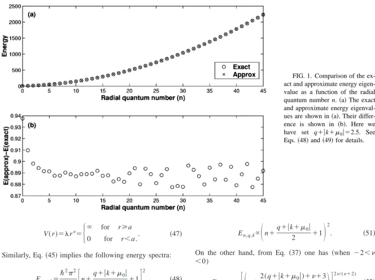
⬁ for r⭓a0 for r⬍a.. 共47兲 Similarly, Eq.共45兲 implies the following energy spectra:
En,q,k⫽ ប22 2ma2
冋
n⫹ q⫹兩k⫹0兩 2 ⫹1册
2 . 共48兲Here we have replaced (n⫹␥/2⫹3/4) with (n⫹␥/2⫹1) ac-cording to the matching condition of the WKB approxima-tion given in the Appendix. The analytic energy spectra of this system are then given by the zeros of the modified Bessel function in Eq.共3.28兲 of the Ref. 关16兴
Iq⫹兩k⫹
0兩⫹1/2
冉
冑
⫺2mEប a
冊
⫽0. 共49兲The numerical analysis shown in Fig. 1共a兲 共for q⫹兩k⫹0兩
⫽2.5) indicates that the result 共48兲 is in good agreement with
the exact result 共49兲. In addition, Fig. 1共b兲 exhibits the dif-ference between the exact and approximate results.
III. THE DEPENDENCE OF THE DISTRIBUTION OF THE ENERGY SPECTRA
Note that Eq.共45兲 indicates that
En,q,k⬀
冉
n⫹ q⫹兩k⫹0兩 2 ⫹ 3 4冊
2/(⫹2) . 共50兲For example, for the model with an infinitely deep potential
共i.e.,→⬁), one has
En,q,k⬀
冉
n⫹q⫹兩k⫹0兩 2 ⫹1
冊
2
. 共51兲
On the other hand, from Eq. 共37兲 one has 共when ⫺2⬍
⬍0) En,q,k⬀⫺
冋冉
n⫹ 2共q⫹兩k⫹0兩兲⫹⫹3 2⫹4冊册
2/(⫹2) . 共52兲 In addition, we can calculate their derivatives with respect to n and find thatEn,q,k
n ⬎0 共53兲
for all considered models. Thus one expects that the energy levels En,q,k will monotonically increase as n increases
monotonically. The q and兩k⫹0兩 dependence of the energy eigenvalue En,q,k can be found by the Hellmann-Feynman
formula 共e.g., 关24兴兲 En,q,k
q ⫽
冓
⌿n,q,k冏
Hq
冏
⌿n,q,k冔
, 共54兲 where the Hamiltonian is given byH⫽⫺ ប 2 2m d2 dr2⫹
冉
r ⫹ ប 2 2m ⫻共q⫹兩k⫹0兩兲共q⫹兩k⫹0兩⫹1兲 r2冊
. 共55兲Thus, we can derive the following results:
FIG. 1. Comparison of the ex-act and approximate energy eigen-value as a function of the radial quantum number n.共a兲 The exact and approximate energy eigenval-ues are shown in共a兲. Their differ-ence is shown in 共b兲. Here we have set q⫹兩k⫹0兩⫽2.5. See
En,q,k q ⫽
冓
⌿n,q,k冏
关2共q⫹兩k⫹0兩兲⫹1兴ប2 2mr2冏
⌿n,q,k冔
⬎0, 共56兲 En,q,k 兩k⫹0兩 ⫽冓
⌿n,q,k冏
关2共q⫹兩k⫹0兩兲⫹1兴ប2 2mr2冏
⌿n,q,k冔
⬎0. 共57兲This means that the energy spectra En,q,kwill monotonically
increase as any one of the quantum numbers in the set (n,q,k) increases monotonically. Therefore the ground state will be given by n⫽q⫽k⫽0. The details can be obtained by analyzing the tendency of En,q,k with respect to the change
of the parameter.
A. Distribution tendency of the energy spectra forÄÀ1
The energy spectra for a charged particle moving in the Coulomb potential and an AB flux is given by Eq. 共38兲. Its first- and second-order derivatives with respect to the param-eters (n,q,兩k⫹0兩) are En,q,k n ⫽mc 2␣2 1 共n⫹q⫹兩k⫹0兩⫹1兲3⬎0, 2E n,q,k n2 ⫽mc 2␣2 ⫺3 共n⫹q⫹兩k⫹0兩⫹1兲4⬍0, 共58兲 En,q,k q ⫽mc 2␣2 1 共n⫹q⫹兩k⫹0兩⫹1兲3⬎0, 2E n,q,k q2 ⫽mc 2␣2 ⫺3 共n⫹q⫹兩k⫹0兩⫹1兲4⬍0, 共59兲 En,q,k 兩k⫹0兩 ⫽mc2␣2 1 共n⫹q⫹兩k⫹0兩⫹1兲3⬎0, 2E n,q,k 兩k⫹0兩2⫽mc 2␣2 ⫺3 共n⫹q⫹兩k⫹0兩⫹1兲 4⬍0. 共60兲
Consequently, En,q,ktends to increase and saturate gradually
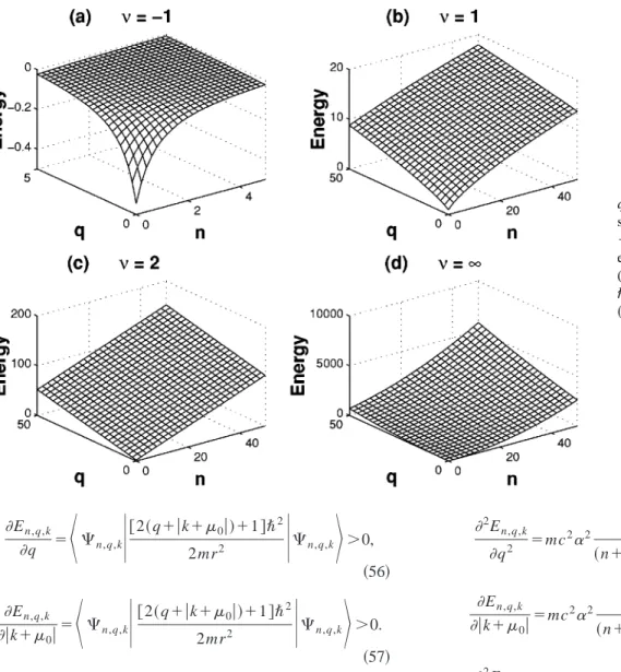
as anyone of the parameters in the set (n,q,兩k⫹0兩) in-creases. It implies the bending curve as shown in Fig. 2共a兲. The unit of the energy eigenvalue in Fig. 2共a兲 is chosen as mc2␣2/2.
B. Distribution tendency of the energy spectra forÄ1
The energy levels for the model with ⫽1 are given by Eq. 共45兲, En,q,k⫽
冉
2ប2 2m冊
1/3冋
3 2冉
n⫹ 共q⫹兩k⫹0兩兲 2 ⫹ 3 4冊册
2/3 . 共61兲Their derivatives with respect to the parameters (n,q,兩k
⫹0兩) yield En,q,k n ⫽
冉
2ប2 2m冊
1/3 冋
32冉
n⫹共q⫹兩k⫹0兩兲 2 ⫹ 3 4冊册
⫺1/3 ⬎0,FIG. 2. Energy as a function of
q and n for four different ’s is
shown. Here we have chosen 兩k
⫹0兩⫽0.5. The unit of the energy
eigenvalue is set as mc2␣2/2,
(922ប2/8m)1/3, ប, and
ប22/2ma2 for 共a兲, 共b兲, 共c兲, and
2E n,q,k n2 ⫽⫺
冉
2ប2 2m冊
1/3冉
2 2冊
⫻冋
32冉
n⫹共q⫹兩k⫹0兩兲 2 ⫹ 3 4冊册
⫺4/3 ⬍0, 共62兲 En,q,k q ⫽冉
2ប2 2m冊
1/3 2冋
3 2冉
n⫹ 共q⫹兩k⫹0兩兲 2 ⫹ 3 4冊册
⫺1/3 ⬎0, 2E n,q,k q2 ⫽⫺冉
2ប2 2m冊
1/3冉
2 8冊
⫻冋
3 2冉
n⫹ 共q⫹兩k⫹0兩兲 2 ⫹ 3 4冊册
⫺4/3 ⬍0, 共63兲 and En,q,k 兩k⫹0兩 ⫽冉
2ប2 2m冊
1/3冉
2冊
⫻冋
3 2冉
n⫹ 共q⫹兩k⫹0兩兲 2 ⫹ 3 4冊册
⫺1/3 ⬎0, 2E n,q,k 兩k⫹0兩2⫽⫺冉
2ប2 2m冊
1/3冉
2 8冊
⫻冋
32冉
n⫹共q⫹兩k⫹0兩兲 2 ⫹ 3 4冊册
⫺4/3 ⬍0 . 共64兲It is obvious that En,q,kwill monotonically increase when the
value of any parameter of the set (n,q,兩k⫹0兩) increases as shown in Fig. 2共b兲. Note that the slope is much more smooth than the model with⫽⫺1. The unit of energy in Fig.2共b兲 is chosen as (922ប2/8m)1/3.
C. Distribution tendency of the energy spectra forÄ2
The energy spectra for a charged particle moving in the three-dimensional harmonic potential and an AB flux is given by Eq.共46兲. Its first- and second-order derivatives with respect to the set of parameters (n,q,兩k⫹0兩) read
En,q,k n ⫽2ប共const兲, 2E n,q,k n2 ⫽0, 共65兲 En,q,k q ⫽ប共const兲, 2E n,q,k q2 ⫽0, 共66兲 and En,q,k 兩k⫹0兩 ⫽ប 共const兲, 2E n,q,k 兩k⫹0兩2⫽0. 共67兲 FIG. 3. Energy as a function of
q and n for four different’s. Here
This means that En,q,kwill linearly increase as any one of the
parameters in the set (n,q,兩k⫹0兩) increases. The details is shown in Fig. 2共c兲 with the unit of energy given by ប.
D. Distribution tendency of the energy spectra forÄⴥ
According to Eq. 共48兲, we obtain the first- and second-order derivatives with respect to En,q,k
En,q,k n ⫽ 2ប2 ma2
冋
n⫹ 共q⫹兩k⫹0兩兲 2 ⫹1册
⬎0, 2E n,q,k n2 ⫽ 2ប2 ma2⬎0, 共68兲 En,q,k q ⫽ 2ប2 2ma2冋
n⫹ 共q⫹兩k⫹0兩兲 2 ⫹1册
⬎0, 2E n,q,k q2 ⫽ 2ប2 4ma2⬎0, 共69兲 and En,q,k 兩k⫹0兩 ⫽ 2ប2 2ma2冋
n⫹ 共q⫹兩k⫹0兩兲 2 ⫹1册
⬎0, 2E n,q,k 兩k⫹0兩2⫽ 2ប2 4ma2⬎0 共70兲for the model with →⬁. Note that En,q,k will increase
monotonically when any one of the parameters in the set (n,q,兩k⫹0兩) increases. The rate of increase is, however, faster than the model ⫽2 since the curve climbs up as shown in Fig. 2共d兲 with the unit chosen as ប22/2ma2.
In summary, all these results imply the following rules for a charged particle moving in the spherically symmetric po-tential V(r)⫽r(⫺2⬍⬍⬁) and an AB magnetic flux.
共a兲 The energy spectra of the bound states depend on the
quantum number (n,q,k) and increase monotonically as any one of the quantum numbers increases.
共b兲 When⫽2, the energy spectra En,q,kdepend linearly
on any parameter in the set (n,q,k); when⬎2, the energy curve bends up as any one of the quantum numbers (n,q,k) increases. On the other hand, when ⬍2, the curve bends down as any one of the quantum numbers increases.
共c兲 When ⫽2, we have E/n:E/q⫽2:1,
E/n:E/兩k⫹0兩⫽2:1, and E/q:E/兩k⫹0兩⫽1:1, which are related to the closeness of the classical orbits and whether the model is exactly solvable or not. For the case with positive power of,
E⬃
冋冉
n⫹共q⫹兩k⫹0兩兲 2 ⫹ 3 4冊册
2/(⫹2) .Although we still have the same ratio of derivatives, the above relation does not hold for the exact solution.
共d兲 When ⫽⫺1, its energy spectra have the properties,
E/n:E/q⫽1:1, E/n:E/兩k⫹0兩⫽1:1, and E/q:E/兩k⫹0兩⫽1:1. They are also related to the closeness of the classical orbits. For models with negative power of,(⫺2⬍⬍0), the WKB approximation given by the Eq.共37兲 implies that
E⬃
冋冉
n⫹2共q⫹兩k⫹0兩兲⫹⫹32⫹4
冊册
2/(⫹2) .
This hence implies that E/n:E/q⫽⫹2,E/ n:E/兩k⫹0兩⫽⫹2, and E/q:E/兩k⫹0兩⫽⫹2 are all equal. This relation does not hold for the exact result for the same reason.
共e兲 The increase in the intensity of the magnetic flux will
change the slope of the energy distribution in both the mod-els with ⫺2⬍⬍0 and the models with 0⬍⬍⬁. More explicitly, when ⬍2, increasing the flux will depress the slope; whereas when ⬎2, increasing the flux will lead to the increase in the slope. In addition, the model with⫽2 is marginal in the sense that the slope of the energy distribution will not be affected by the change of the flux. For details, see the difference shown in the Figs. 2 and 3. Note that 兩k
⫹0兩 is set as 0.5 and 12 in Figs. 2 and 3, respectively. IV. CONCLUSION
The semiclassical quantization rule is presented for a charged particle moving in a system with a general central force described by the potential V(r)⫽r, with ⫺2⬍
⬍⬁, and an AB magnetic flux. The formulas obtained in this
paper are in good agreement with the energy levels with all known exactly solvable models with some specific values of . Furthermore, we have presented numerical results for
⫽⬁, which are also in good agreement with the exact result.
Therefore, one expects that the semiclassical quantization rules will also be in good agreement with the models pre-scribed by a large ranges of even the results shown in this paper are more reliable for the case with large principle quantum number n.
APPENDIX
The WKB wave function for a charged particle moving in a smooth potential well near the neighborhood x⬃a(x⬎a), where x⫽a,b are the intersection points of the horizonal line y⫽E and the curve y⫽V(x) as shown in Fig. 4共a兲, can be FIG. 4. WKB wave function matching boundary conditions for three cases of potentials.
expressed in terms of the classical momentum p as共see, for example, Ref.关24兴 for details兲
⌿共x兲⫽
冑
C psin冋
1 ប冕
a x pdx⫹ 4册
⬅ C冑
psin␣共x兲, 共A1兲 where C is constant. Analogously, near the neighborhood x⬃b (x⬍b) we have ⌿共x兲⫽
冑
C⬘
psin冋
1 ប冕
x b pdx⫹ 4册
⬅ C⬘
冑
psin共x兲. 共A2兲 These two wave functions must be consistent. This means that near the neighborhoods a,b of x,␣共x兲⫹共x兲⫽1ប
冕
a b pdx⫹ 2⫽共n⫹1兲,n⫽0,1,2,3, . . . . 共A3兲 Or equivalently,冖
pdx⫽冉
n⫹1 2冊
h,n⫽0,1,2,3, . . . . 共A4兲 For the half-infinite potential well as shown in Fig. 4共b兲, one has冖
pdx⫽冉
n⫹34
冊
h,n⫽0,1,2,3, . . . . 共A5兲 Analogously, the matching rule of the wave functions gives the quantization rule for the system with an infinitely deep square-well potential as illustrated in Fig. 4共c兲. Indeed, one has冖
pdx⫽共n⫹1兲h,n⫽0,1,2,3, . . . . 共A6兲The argument leading to the same result for a more general condition beyond the above examples can be found with the help of the Maslov index shown in Ref.关25兴.
关1兴 M.G. Alford and F. Wilczek, Phys. Rev. Lett. 62, 1071 共1989兲. 关2兴 D. Deser, R. Jackiw and G. ’tHooft, Ann. Phys. 共Paris兲 152, 220 共1984兲; S. Deser and R. Jackiw, Commun. Math. Phys.
118, 495共1988兲; P. de Sousa Gerbert and R. Jackiw, ibid. 124,
229共1989兲.
关3兴 F. Wilczek, Phys. Rev. Lett. 49, 957 共1982兲; Y.H. Chen, F. Welczek, E. Witten and B.I. Halperin, Int. J. Mod. Phys. B 3, 1001共1989兲.
关4兴 Z.F. Ezawa, M. Hotta, and A. Iwazaki, Phys. Rev. D 44, 3906 共1991兲.
关5兴 C.A. Trugenberger, Phys. Rev. D 45, 3807 共1992兲.
关6兴 R.B. Laughlin, Phys. Rev. B 23, 3383 共1983兲; F.D.M. Haldane, Phys. Rev. Lett. 51, 605共1983兲; B.I. Halperin, ibid. 52, 1583 共1984兲.
关7兴 Z.F. Ezawa and A. Iwazaki, Phys. Rev. B 43, 2637 共1991兲. 关8兴 R.B. Laughlin, Phys. Rev. Lett. 60, 1057 共1988兲; A. Fetter, C.
Hanna, and R.B. Laughlin, Phys. Rev. B 39, 9679共1989兲. 关9兴 I.V. Barashenkov and A.O. Harin, Phys. Rev. Lett. 72, 1575
共1994兲; Phys. Rev. D 52, 2471 共1995兲.
关10兴 A. Guha and S. Mukherjee, J. Math. Phys. 28, 840 共1987兲; M. Kibler, and T. Negadi, Phys. Lett. A 124, 42 共1987兲; G.E. Draganascu, C. Campigotto, and M. Kibler, ibid. 170, 339 共1992兲; V.M. Villalba, ibid. 193, 218 共1994兲; L. Chetonani, L. Guechi, and T.F. Hamman, J. Math. Phys. 30, 655共1989兲.
关11兴 D.H. Lin, J. Phys. A , 4785 共1998兲; J. Math. Phys. 40, 1264 共1999兲.
关12兴 Q.G. Lin, Phys. Rev. A 59, 3228 共1999兲.
关13兴 M. C. Gutzwiller, Chaos in Classical and Quantum Mechanics 共Springer Verlag, New York, 1990兲.
关14兴 V.M. Strutinsky, Nukleonika 20, 679 共1975兲; V.M. Strutinsky and A.G. Manger, Elem. Part. & Nucl.共Atomizdat, Moscow兲
7, 356共1976兲 关Sov. J. Part. Nucl. 7, 138 共1976兲兴.
关15兴 M. Brack and R. K. Bhaduri, Semiclassical Physics 共Addison-Wesley, New York, 1997兲.
关16兴 D.S. Chuu and D.H. Lin, J. Phys. A 34, 2561 共2001兲. 关17兴 C.N. Yang, Phys. Rev. Lett. 33, 445 共1974兲.
关18兴 T.T. Wu and C.N. Yang, Phys. Rev. D 12, 3845 共1975兲. 关19兴 D.H. Lin, J. Math. Phys. 41, 2723 共2000兲.
关20兴 D.H. Lin, Ann. Phys. 共N.Y.兲 290, 1 共2001兲.
关21兴 H. Kleinert, Path Integrals in Quantum Mechanics, Statistics and Polymer Physics共World Scientific, Singapore, 1995兲. 关22兴 J. Y. Zeng, Problem in Quantum Mechanics 共Science Press,
Beijing, 1988兲.
关23兴 W. Magnus, F. Oberhettinger, and R. P. Soni, Formulas and Theorems of the Special Function of Mathematical Physics 共Springer, Berlin, 1966兲.
关24兴 J. Y. Zeng, Quantum Mechanics 共Science Press, Beijing, 1999兲.
关25兴 H. Kleinert and D.H. Lin, e-print quant-ph/9807068; D.H. Lin, e-print quant-ph/9901049.