一個創新的平行蜂群演算法實作在圖形處理器架構

國

立

交

通

大

學

資訊科學與工程研究所

碩

士

論

文

一 個 創 新 的 平 行 蜂 群 演 算 法

實

作

在

圖

形

處

理

器

架

構

A novel parallel Bees Algorithm for optimization problems on

GPU

研 究 生：黃聖凱

指導教授：袁賢銘 教授

一個基於圖形處理器的平行式蜂群演算法

用以解決最佳化問題

A novel parallel Bees Algorithm for optimization problems on

GPU

研 究 生：黃聖凱 Student：Sheng-Kai Huang

指導教授：袁賢銘 Advisor：Shyan-Ming Yuan

國 立 交 通 大 學

資 訊 科 學 與 工 程 研 究 所

碩 士 論 文

A Thesis

Submitted to Department of Computer and Information Science

College of Electrical Engineering and Computer Science

National Chiao Tung University

in partial Fulfillment of the Requirements

for the Degree of

Master

in

Computer and Information Science

June 2012

i

一個創新的平行蜂群演算法

實作在圖形處理器架構

研究生：黃聖凱 指導教授：袁賢銘 國立交通大學資訊科學與工程研究所碩士班 摘要 尋求最佳解在電腦科學或和其他工程領域裡面是很重要的一環，然而尋求最佳 解屬於 NP 問題，取而代之去尋近似最佳解的演算法也越來越多。Swarm Intelligence 是 透過觀察大自然中社會型動物的生活方式應用在人工智慧來解決問題，蜂群演算法就是 其中一個。由於找尋近似最佳解的演算法也 CPU bound job，一些平行處理的演算法也 因此相繼被人提出，到目前為止，鮮少人關心蜂群演算法的平行化。

圖形處理器(GPU)是專門針對圖形處理而設計的架構，因為影像處理具備高度 平行化的特性，造就了 GPGPU 的發展，許多的研究也開始利用 GPU 進行大量的平行運 算。近年， 由 NVIDIA 提出 GPGPU 的 解 決方案 CUDA(Compute Unified Device Architecture)讓開發者利用熟悉的 C/C++就可以在上面開發自己的平行應用程式。

本論文針對需要大量運算的蜂群演算法提出許多方法使其平行化且適合在 CUDA 的平行架構運行，並針對幾個知名的最佳化問題做了效能上面的測試。根據我們的實驗 結果，可以發現平行化的 CUDA Bees Algorithm (CUBA) 利用龐大數量的處理器，在各 個最佳化問題比起傳統的 Bees Algorithm(BA)至少有 3X 倍效能的加速。

ii

A novel parallel Bees Algorithm for optimization problems on

GPU

Student: Sheng-Kai Huang Advisor: Shyan-Ming Yuan

Department of Computer Science and Engineering

National Chiao Tung University

Abstract

Searching the solution of optimization problems is a very important work in computer

science and engineering field. The problems are belong to NP problem, so more and more

algorithms are developed to find approximate solutions instead of the real solutions. Swarm

Intelligence is the collective behavior of the system of social animals in nature. The concept is

used in algorithm on artificial intelligence(AI). The Bees Algorithm is one of the works.

Because these algorithms are computational bound jobs, some parallel swarm based

algorithms are proposed in recent years. Even so, few works are developed base on The Bees

Algorithm.

GPU is a special architecture of graphic processor. The highly parallel features of

graphic processing made the rapid development of General Purpose GPU(GPGPU). A lot

works for massive parallel computing on GPU are proposed. NVIDIA provide a general

purpose parallel model, thus programmer could use their familiar language C/C++ to develop

own parallel applications.

In this paper, we do many modifications for The Bees Algorithm and make it adapt to run

in the parallel architecture of CUDA. We also test the performance accelerations for numerous

famous optimization problems. Finally, the result shows the CUDA Bees Algorithm(CUBA)

we proposed perform at least 3x times faster than traditional BA in numerous different

iii

Acknowledgement

碩士班生涯是我最重要的人生過程之一，很慶幸加入分散式系統實驗室。非常感謝 我的指導教授袁賢銘老師這兩年來對我不厭其煩的教導，老師開明且自由的指導方式，讓 我能夠在碩士班期間學到不少專業領域的相關知識，老師充分給予學生想法揮灑的空間， 也會耐心的給予各種寶貴的建議。在這兩年，無論是大大小小的程式競賽，或是研究計畫 ，甚至在找工作方面，老師給我非常多的幫助，讓我能夠順利完成這些任務。實驗室方面 非常感謝國亨學長在這期間，在我研究遇到瓶頸挫折的時候，給予我一些專業的方向，刺 激我的思考，讓我能夠走過低潮，也感謝永威學長、家峰學長以及江川彥不吝在各個方面 提供我幫助。感謝我實驗室的同學們紘維、冠穎、珮瑜在這兩年陪伴，不論在課業上，研 究上，生活上讓我能夠學習成長。孟傑、俊凱在這一年的加入，讓實驗室更加的歡樂、溫 馨。學弟們先博、柏志、振庭、丞訓讓實驗室充滿著朝氣，每個禮拜的球聚，以及不定期 的餐聚，凝結著我們DCSLAB團結的心。感謝實驗室的大家帶給我歡笑與成長。在最後我要 感謝我的家人，沒有你們，就沒有今天的我，有了你們的支持，我的人生過得很充實。

iv

Table of Contents

Acknowledgement ... iii Table of Contents ... iv List of Table ... v List of Figures ... vi Chapter 1 Introduction ... 1 1.1Preface ... 1 1.2Motivation ... 1 1.3Research Objective ... 2 1.4Research Contribution ... 2

Chapter 2 Background and Related Work ... 3

2.1Optimization problems ... 3

2.2Intelligent swarm-based optimization Algorithm ... 3

2.3The Bees Algorithm ... 4

2.4General Purpose Computation on GPU ... 6

2.5Compute Unified Device Architecture (CUDA) ... 9

2.6 Related Work ... 11

2.6.1 Parallel Bees Algorithm for ATC Enhancement in Modern Electrical Network ... 11

Chapter 3 Parallel Bees Algorithm on GPU ... 12

3.1System Overview ... 13

3.2Parallel Approaches ... 13

3.2.1 Parallel Initialization ... 14

3.2.2 Odd–Even Sort ... 14

3.2.2 Group Bees into Different Colonies ... 16

3.2.3 Modified Bees Algorithm ... 16

v

4.1 Evaluation Environment ... 19

4.2 Benchmark Functions ... 19

4.3 Analysis and Result ... 30

4.3.1 Analysis of nep ... 31

4.3.2 Analysis of the number of colonies ... 32

4.3.3 Analysis of the number of bees ... 34

4.3.4 Robustness and Speedup ... 35

Chapter 5 Conclusion and Future work ... 39

Reference ... 41

Appendex ... 43

source code: cuba.h ... 43

source code: cuba.cu ... 44

List of Table

Table 3 - 1 Odd-Even Sort Algorithm ... 15

Table 4 - 1 Hardware configurations ... 19

Table 4 - 2 Benchmark Functions... 29

Table 4 - 3 nep increasing (time) ... 31

Table 4 - 4 nep increasing (iterations) ... 32

Table 4 - 5 colonies increasing (time) ... 33

Table 4 - 6 colonies increasing (iterations) ... 33

Table 4 - 7 bees increasing (time) ... 34

Table 4 - 8 bees increasing (iterations) ... 34

Table 4 - 9 Combinations of Bees Algorithm parameters ... 35

Table 4 - 10 Combinations of CUDA Bees Algorithm parameters ... 36

Table 4 - 11 The successful rate in 50 runs ... 37

Table 4 - 12 Speedups ... 38

vi

List of Figures

Figure 2 - 1 Flowchart of the basic Bees Algorithm [6] ... 5

Figure 2 - 2 The comparison of computation power between CPU and GPU . .. 7

Figure 2 - 3 Floating-Point Operations per second and memory bandwidth for the CPU and GPU [11] ... 8

Figure 2 - 4 The GPU Devotes More Transistors to Data Processing [12] ... 9

Figure 2 - 5 hardware viewpoint of CUDA architecture ... 10

Figure 2 - 6 Software viewpoint of CUDA architecture ... 10

Figure 2 - 7 (a)Serial Approach (b)Parallel Approach [21] ... 11

Figure 2 - 8 Comparison of Elapsed Time for Different Algorithms in seconds [21] ... 12

Figure 3 - 1 Framework of the CUBA ... 13

Figure 3 - 2 Algorithm of the CUBA ... 14

Figure 3 - 3 Procedure of Odd-Even Sort ... 15

Figure 4 - 1 The surface plot of Ackley’ function ... 20

Figure 4 - 2 The surface Easom function ... 21

Figure 4 - 3 The surface Gold and Price function ... 22

Figure 4 - 4 The surface Martin and Gaddy function ... 23

Figure 4 - 5 The surface Schaffer function ... 24

Figure 4 - 6 Schewefel function ... 25

Figure 4 - 7 The surface Hyper Sphere function ... 26

Figure 4 - 8 Griewank function ... 27

1

Chapter 1 Introduction

1.1 Preface

Optimization problems have been the subject of much research in recent years. It’s a

NP-problem, so many different alternative techniques have been developed. The swarm

intelligence is one of those methods which is used to solve the near optimal solution. Many

researchers have introduced various algorithms by modeling the behaviors of the swarm of

animals in nature [1-5]. Self-organization is the feature of the system which gets global-level

response by means of many different low-level interactions.

The Bees Algorithm was proposed by DT Pham [1] in 2005 for optimizations problems,

and the improved performance of the algorithm have been proposed several years latter [6].

Researchers have come up with several real-word applications such as data mining [7], robot

controlling [8], electronic engineering [9], job scheduling for the Bees Algorithm [10].

1.2 Motivation

Because of the optimization problems are computational issues, we want to find a

parallel way that can speed up the Bees Algorithm. Nowadays modern Graphic Processing

Units (GPU), which can be seen as highly fast parallel general-purpose systems. Developers

have designed many algorithms and applications on GPU for better performance. Moreover,

several general purpose languages for GPUs have become popular such as CUDA [11, 12]. It

supports many graphic programming APIs, so developers do not have to consider more

complexity of low-level problems while programming with CUDA. Although much work has

be done on developing parallel swam intelligence algorithm on GPU such as Ant Colony

2

develop the parallel bees algorithm on GPU. The purpose of this paper is to develop a novel

parallel Bees Algorithm which is adapt running on GPU.

1.3 Research Objective

For the reasons we mentioned above, we implemented a parallel Bees Algorithm to test

the speedup for several common functions of optimizations problems. We evaluated and

compared both of the execution time with CUDA on GPU and the execution time with C++

on CPU to verify efficiency of the algorithm.

1.4 Research Contribution

The following are our research contributions:

1. A novel parallel Bees Algorithm on GPUs

3

Chapter 2 Background and Related Work

2.1 Optimization problems

The standard form of a (continuous) optimization problem is

where

 is the objective function to be minimized over the variable ,  are called inequality constraints, and

 are called equality constraints.

By convention, the standard form defines a minimization problem. A maximization

problem can be treated by negating the objective function.[18-20]

2.2 Intelligent swarm-based optimization Algorithm

Many complex multi-valuable optimization problems can’t be solved within polynomial

computation times. For the reason, many researchers interested in search algorithms which

finding approximate optimal solutions in reasonable running time. Swarm intelligence is the

field of optimization and researchers have developed various algorithms by modeling the

behaviors of different swarm animal with social organization such as ants, bees, birds…and so

on. In 1990s, Those algorithm inspired by ants like Ant Colony Optimization had been

proposed by Marco Dorigo [1]. Kennedy also developed the Particle swarm optimization

(PSO) [3]. Those algorithm inspired by honey bees such as The Bees Algorithm by DT Pham

4

2.3 The Bees Algorithm

The Bees Algorithm is population-based method to search optimization of the problems

which is inspired by the behavior of honey bees in nature[2, 6]. It requires several parameters

to be set as following: n (number of scout bees), m (number of sites to be selected from n

visited sites), nep(number of bees recruited for top e sites from the m visited sites),

nsp(number of bees recruited for the other (m-e) selected sites), ngh initial size of patches

which includes site and its neighbourhood and stopping criterion. The algorithm begins with

the n scout bees which randomly being placed in the searching domain. The basic Bees

Algorithm is shown in following and the corresponded flowchart is in Figure 2-1

1. Initialize populations with random solutions.

2. Evaluate Fitness of the population.(see the fig.)

3. While(the stopping criterion is not met)

//Forming new population.

4. Select sites for neighbourhood search.

5. Recruit bees for selected sites( nep bees for top e sites and nsp bees for remain (m-e) sites)

and evaluate fitness.

6. Select the fittest bee from each patch.

7. Assign remaining bees (n-m) to search randomly and evaluate fitness.

5

Figure 2 - 1 Flowchart of the basic Bees Algorithm [6]

The Bees Algorithm above is the most basic version. Pham DT proposed an improved

version for the Bees Algorithm that increases the search accuracy and avoid superfluous

computations in 2009. Two new procedures were introduced as follows:

1. neighbourhood shrinking

The size of ngh is initially set to a large value as following:

ngh(0) = (maxV - minV)

where the maxV, minV means the max and min searching site in the global area. The local

search is initially defined over a large neighbourhood (equal to the range of the global

search ), and has largely explorative feature. The local search procedure finds any better

site with higher fitness, it keeps the size of ngh unchanged. If no improvement during the

6 ngh(i+1) = 0.8 *ngh(i) if no improvement

ngh(i+1) = ngh(i) else

2. Site abandonment

When no fitness improvement after a number of times (stlim) local search even by

neighbourhood shrinking method, it means the local search procedure perhaps to reach the

top of the local fitness peak, in other words, no further progress will be made. For

efficiency, the exploration of the patch is stopped. If no better fitness of other site is

generated during the remaining random search procedure then abandons this site.

Although there are several researchers come up with new models based on honeybees our

work is based on this model proposed by Pham DT.

2.4 General Purpose Computation on GPU

GPGPU is the use of a GPU (graphic processing unit) as a co-processor to accelerate

GPUs for general purpose scientific and engineering computing .

The GPU accelerates computations and applications running on the CPU by loading part

of the code with high compute-loading. The rest of the code is runs on CPU. To accelerating

application by using the massively parallel processing power of the GPU to get high

7

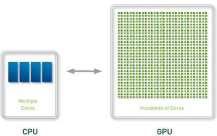
Figure 2 - 2 The comparison of computation power between CPU and GPU .

As illustrated by Figure 2-2, nowadays a CPU consists of 4 to 8 cores while the GPU

consist of hundreds of cores. They cooperate with each other in the application. The

massively parallel computing architecture gives the application higher performance.

GPUs now offer much faster floating-point calculation than CPU as illustrated by Figure

2-3, moreover, several high-level languages for GPGPU such as CUDA and OPENCL have

developed for programmers. The main difference between CPU and GPU is that the GPU is

specialized for compute-intensive, highly parallel computations, GPU devotes more

transistors to process data rather than to cache data and flow control as illustrated by Figure

8

Figure 2 - 3 Floating-Point Operations per second and memory bandwidth for the CPU and GPU [11]

9

Figure 2 - 4 The GPU Devotes More Transistors to Data Processing [12]

2.5 Compute Unified Device Architecture (CUDA)

NVIDIA provides CUDA that is a general purpose parallel programming model, thus the

programmers don’t need to consider the complex low-level issues of GPU. What they have to concern is how to design an parallel algorithm for their applications. The CUDA

programming model provides various languages including C/C++ for developers.

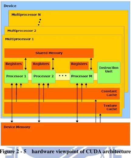
From the perspective of hardware, A GPU consists of a number of multiprocessors, there are

many stream processors in a multiprocessor and each stream processor is a smallest

computational unit. There is shared memory in a multiprocessor among numerous stream

processors, they could communicate by using shared memory. In addition to shared memory,

other types of memory like constant memory, texture memory that could be used in different

situations. Figure 2-5 is a diagram of the hardware viewpoint of CUDA architecture.

From the perspective of software, the code running sequentially on CPU is called “Host” and

the code running paralleled on GPU is called “Kernel”. A kernel is launched as a grid of thread blocks, the thread blocks are executed on multiprocessors. The software viewpoint of

10

Figure 2 - 5 hardware viewpoint of CUDA architecture

11

2.6 Related Work

2.6.1 Parallel Bees Algorithm for ATC Enhancement in Modern

Electrical Network

The paper has proposed a parallel Bees Algorithm for determining the optimal allocation

of FACTS devices[21]. The PAB(parallel Bees Algorithm) simultaneously for nearby searches.

In PAB computations are distributed among the CPUs by matlab workers, thus it’s faster to search a solution and getting better accuracy of solution compared to other technique. It’s the first application of parallel Bees Algorithm in application of FACT devices. The method to

parallel the algorithm is to distribute the computations of evaluating fitness, and the main

difference between serial and parallel approach is shown in Figure 2-7. When they compared

the elapsed time for the application on Intel Quad Core Q6600 running at 2.4GHz system in

matlab 7 environment, the result is illustrated by the Figure 2-8 and getting 2~4 times better.

(a) (b)

12

Figure 2 - 8 Comparison of Elapsed Time for Different Algorithms in seconds [21]

Chapter 3 Parallel Bees Algorithm on GPU

The key that decides the accelerated effect is the level of parallelization. In the traditional

Bees Algorithm, the most computational loading is in neighbourhood search procedure. A

naïve method is to take the neighbourhood search procedure as a kernel to distribute the

computations in loop of the procedure. In fact, the optimal number of the neighbourhood size

is fluctuant according to different features of functions. However, if the size of the

neighbourhood is not larger than number of the total threads within the GPU then the

accelerated effect would not be obvious. Another common solution is “multi-colonies” that

means we should run many Bees Algorithms independently in each threads. There are two

major disadvantages. The first disadvantage is each thread contains many conditional branch,

we could not avoid the divergent branch, so the overhead would be too expensive. The second

one is that the communication among the threads after a round would be more complex to do.

For these reasons, we design a new Bees Algorithm of parallel multi-colonies that bring good

13

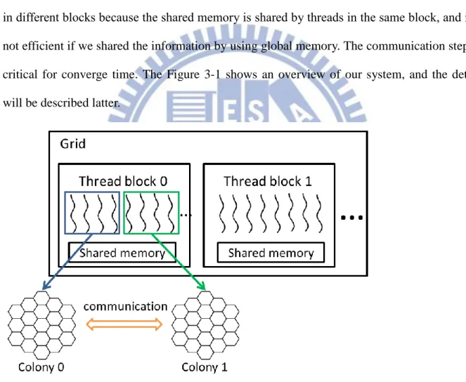
3.1 System Overview

We choose CUDA framework to implement our multi-colonies Bees Algorithm on GPU

called CUBA. In our algorithm, we group the threads within a block to several colonies. To

explain clearly, each thread is assigned to a honey bee to search the solution for its colony. We

divide a block into different colonies by thread ID, and running Bees Algorithm independently.

When one iteration finished, we will change the information between colonies in the same

block by using shared memory. The colonies will not communicate with each other if they are

in different blocks because the shared memory is shared by threads in the same block, and it’s not efficient if we shared the information by using global memory. The communication step is

critical for converge time. The Figure 3-1 shows an overview of our system, and the detail

will be described latter.

Figure 3 - 1 Framework of the CUBA

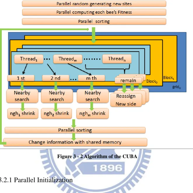
3.2 Parallel Approaches

To parallel The Bees Algorithm, we have overcome many issues. Our CUDA bees algorithm shows in Figure 3-2, and the detail will be explained in this section.

14

Figure 3 - 2 Algorithm of the CUBA

3.2.1 Parallel Initialization

In BA approach, the initialization of population and the evaluation of the fitness of the

population achieve one after one whereas CUBA distributes and computes them among the

threads of GPU. Ideally, it accelerates times of the numbers of threads for this procedure.

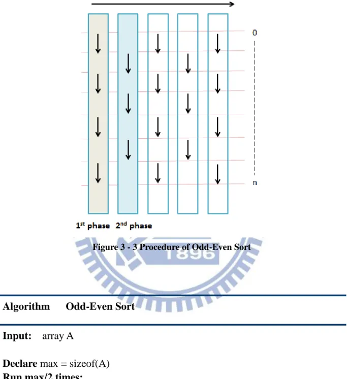
3.2.2 Odd–Even Sort

It’s necessary to sort the fitness of all populations to get the best m sites. Because the size of the sorting data in this application is small respect to others, we sort the colonies in the

same block individually by using Odd–Even Sorting algorithm [22, 23] that is based on the

15

This method only requires n/2 iterations of the two phase sort. The procedure diagram of

Odd-Even Sorting in Figure 3-3 and the algorithm in Table 3-1

Figure 3 - 3 Procedure of Odd-Even Sort

Algorithm Odd-Even Sort

Input: array A

Declare max = sizeof(A)

Run max/2 times:

For i is odd and i < max do in parallel:

If A[i] > A[i+1] then swap(A[i], A[i+1])

For i is even and i < max do in parallel:

If A[i] > A[i+1] then swap(A[i], A[i+1])

Output: sorted array A

16

3.2.2 Group Bees into Different Colonies

We divide threads in the blocks to different colonies according to their thread ID, each

thread is assigned to a honey bee and searching the solution for its colony, so there are a

number of colonies run Bees Algorithm parallel. The number of bees and colonies in the

algorithm is depending on what the number of blocks per grid and number of threads per

block we set.

The number of colonies in a block = number of threads per block / number of bees per colony.

3.2.3 Modified Bees Algorithm

3.2.3.1 Modification of local search

The local search in traditional BA approach, more bees (nep) recruit for elite sites and

fewer bees (nsp) recruits for the rest of sites from e sites. It’s reasonable because the mechanism is based on probability. But in our system, we just assign nep bees to recruit m

sites for balancing the loading among the threads, to be more precisely, it’s not make sense in parallel architecture if some threads would do nothing after finishing their jobs and waiting

for the others.

3.2.3.2 Random Seeds

We have different threads in GPU with different random seeds, so we get more random

effect.

3.2.3.3 Neighbourhood Shrinking

According to the new procedure “neighbourhood shrinking” in BA, ngh constantly

17

simultaneously for parallelism, and we let the recruited bees in different sites with different

ngh. Another adjust is that we don’t need to set a such large number of the recruited bees like in BA, because we have so numerous colonies to search simultaneously that the risk which

may cause wrong shrink we accept is much lower. In the meanwhile, the rapid decreasing of

ngh could bring a faster converge time. What shrinking equation we use is the same with the

equation in the Bees Algorithm. Initially, the size of ngh is set to a large value.

3.2.3.4 Communication with shared memory

In general parallel architectures may use shared memory or message passing method to

communicate between the multiple processing units. There is a shared memory in the same

block in CUDA architecture, so we use it to implement the communication in the end of the

each iteration. In this strategy, there are three issues we have to concern. The first is what

information to share, the second one is who to share with, and the last is how long to

communicate once.

We had tried and compared several mechanisms for communication. For example, we

sort the best results which are gained from individual colonies in the same block after

neighbourhood search, and sharing the best to others. To explain in detail, the site with lowest

fitness in each colony is replaced by best one with highest fitness in the block. The result

shows that converge rate is quite good. However, a sorting procedure often impact on the

execution time, finally, we develop the two-phase communication that avoiding sorting and

with good converge rate, too. The paired exchange take few time to share, and the second

phase improve the global convergence over time. The method is shown as follow:

Adjacent exchange (first phase):

If colony ID is odd, then exchange with colony (ID+1) % number of colonies per block

If colony ID is even, then exchange with colony (ID-1) % number of colonies per block

18

If colony ID is odd, then exchange with colony (ID+2) % number of colonies per block

If colony ID is even, then exchange with colony (ID-2) % number of colonies per block

19

Chapter 4 Experimental Results and Analysis

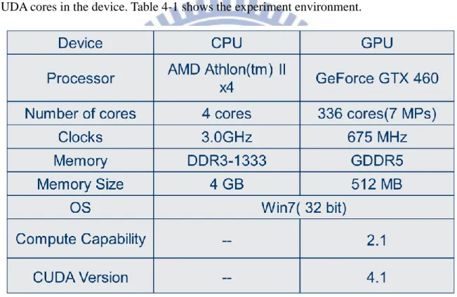
4.1 Evaluation Environment

We adopt AMD Athlon (tm) II and GeForce GTX 460 for our computation platform. The

configuration information is described as following. The host is AMD Athlon(tm) II which

has 4 cores, and each core has clock rate with 3.0GHz. The device is GeForce GTX 460

which has 7 multiprocessors (MPs) and each MP has 48 CUDA cores. Totally, there are 336

CUDA cores in the device. Table 4-1 shows the experiment environment.

Table 4 - 1 Hardware configurations

4.2 Benchmark Functions

Table 4-2 shows the equations of 9 continuous function minimization benchmarks. The

equations are given together with the range of the variables and global minimum. These

functions are widely used multi-modal test functions. The definitions and surface graphs of

20 Ackley function: f(𝑥1, 𝑥2) = 20 − 20𝑒 −0.2√1₂₍𝑥₁2+𝑥₂2) − 𝑒12 [cos(2𝜋𝑥1)+cos(2𝜋𝑥2)]_{+ 𝑒 , −32 < 𝑥} 𝑖 < 32

21 Easom function: 𝑓(𝑥1, 𝑥2) = − cos(𝑥1) ∗ cos (𝑥2) 𝑒−(𝑥1−𝜋) 2_{− (𝑥} 2−𝜋)2, −100 < _𝑥 𝑖 < 100

22

Goldstein and Price function

A(𝑥1, 𝑥2) = 1 + (𝑥1+ 𝑥2+ 1)2(19 – 14𝑥1+ 3𝑥12− 14𝑥2+ 6𝑥1𝑥2+ 3𝑥22)

B(𝑥1, 𝑥2) = 30 + (2𝑥1− 3𝑥2)2(18 − 32𝑥1+ 12𝑥12+ 48𝑥2− 36𝑥1𝑥2+ 27𝑥22)

𝑓(𝑥1, 𝑥2) = 𝐴𝐵, −2 < 𝑥𝑖 < 2

23

Martin and Gaddy function

𝑓(𝑥1, 𝑥2) = (𝑥1− 𝑥2)2+ [

(𝑥1+𝑥2− 10 )

3 ]2 , −20 < 𝑥𝑖 < 20

24 Schaffer function 𝑓(𝑥1, 𝑥2) = 0.5 + [sin(√𝑥12+𝑥22)]2− 0.5 [1.0 + 0.001(𝑥12+𝑥12)]2 , −100 < 𝑥𝑖 < 100

25

Schwefel function

𝑓(𝑥1, 𝑥2) = −𝑥1sin (√|𝑥1|−−𝑥2sin(√|𝑥2|),−500 < 𝑥𝑖 < 500

26 Hyper Sphere 𝑓(𝑥⃗) = ∑𝑥𝑖2 10 𝑖=1 , −100 < 𝑥𝑖 < 100

27 Griewank 𝑓(𝑥⃗) = 1 4000 ∑(𝑥𝑖 − 100) 2 _−∏cos(𝑥𝑖− 100 √𝑖 + 1 )+ 1,−600 < 𝑥𝑖 < 600 10 𝑖=1 10 𝑖=1

28 Rosenbrock function 𝑓(𝑥⃗) = ∑ 100(𝑥_𝑖+1− 𝑥𝑖2) 2 + (1 − 𝑥𝑖)2 9 𝑖=1 , −50 < 𝑥𝑖 < 50

29

Function Equation Minimum

Ackley(2D) 𝑓(𝑥1, 𝑥2) = 20 − 20𝑒 −0.2√1₂₍𝑥12+𝑥22)_{− 𝑒}1_{2 [cos(2𝜋}𝑥₁)+cos(2𝜋𝑥₂)]_{+ 𝑒 , −32} < 𝑥𝑖 < 32 𝑥⃗= (0⃗⃗) f(𝑥⃗) = 0 Easom(2D) 𝑓(_{𝑥1, 𝑥2}) = − cos(_𝑥1) ∗ cos (_𝑥2) 𝑒−(𝑥1−𝜋)2− (𝑥2−𝜋)2, −100 <_𝑥

𝑖 < 100 𝑥⃗= (𝜋, 𝜋)

f(𝑥⃗) = −1 Goldstein and Price(2D) A(𝑥1, 𝑥2) = 1 + (𝑥1+ 𝑥2+ 1)2(19 – 14𝑥1+ 3𝑥12− 14𝑥2+ 6𝑥1𝑥2+ 3𝑥22)

B(𝑥1, 𝑥2) = 30 + (2𝑥1− 3𝑥2)2(18 − 32𝑥1+ 12𝑥12+ 48𝑥2− 36𝑥1𝑥2+ 27𝑥22)

𝑓(𝑥1, 𝑥2) = 𝐴𝐵, −2 < 𝑥𝑖 < 2

𝑥⃗= (0, −1) f(𝑥⃗) = 3

Martin and Gaddy(2D) _𝑓(

𝑥1, 𝑥2) = (𝑥1− 𝑥2)2+ [ (𝑥1+𝑥2− 10 ) 3 ]2 , −20 < 𝑥𝑖 < 20 𝑥⃗= (5, 5) f(𝑥⃗) = 0 Schaffer(2D) 𝑓(𝑥1, 𝑥2) = 0.5 + [sin(√𝑥12+𝑥22)]2− 0.5 [1.0 + 0.001(𝑥12+𝑥12)]2 , −100 < 𝑥𝑖 < 100 𝑥⃗= (0⃗⃗) f(𝑥⃗) = 0 Schwefel(2D) _𝑓(𝑥 1, 𝑥2) = −𝑥1sin (√|𝑥1|−−𝑥2sin(√|𝑥2|),−500 < 𝑥𝑖 < 500 𝑥⃗= (420.97⃗⃗⃗⃗⃗⃗⃗⃗⃗⃗⃗⃗⃗⃗⃗) f(𝑥⃗) = −837.97 Hyper Sphere(10D) 𝑓(𝑥⃗) = ∑𝑥𝑖2 10 𝑖=1 , −100 < 𝑥𝑖 < 100 𝑥⃗= (0⃗⃗) f(𝑥⃗) = 0 Griewank(10D) 𝑓(𝑥⃗) = 1 4000 ∑(𝑥𝑖− 100) 2 10 𝑖=1 −∏cos(𝑥𝑖− 100 √𝑖 + 1 )+ 1,−600 < 𝑥𝑖 < 600 10 𝑖=1 𝑥⃗= (100⃗⃗⃗⃗⃗⃗⃗⃗) f(𝑥⃗) = 0 Rosenbrock(10D) 𝑓(𝑥⃗) = ∑9_𝑖=1100(𝑥_𝑖+1− 𝑥_𝑖2)2+ (1 − 𝑥_𝑖)2, −50 < 𝑥𝑖 < 50 𝑥⃗= (0⃗⃗) f(𝑥⃗) = 0

30

4.3 Analysis and Result

For CUBA, there are 5 parameters we have to set, GridDim, BlockDim, N, M and nep.

In CUDA programming, the code running parallel is called “kernel”, the job size of kernel is

so called “grid”. The programmer should set a dimensional number of grid. CUDA will divide

the job to many smaller jobs and distribute them to different multiprocessors to execute. The

size of each smaller job is called “block”. As setting dimensional number of grid, the

programmer has to set the dimensional number of block, meaning how many threads in a

block. In our algorithm, there are BlockDim / N colonies per block. For example if we set

BlockDim = 256 and N = 8, then there are 32 colonies in a block. The parameters are set

according to the results of the experiments in the next chapter, we will discuss in more detail

later.

All the programs both of BA and CUBA in the following experiments were run until

either the minimum of the function was approximated to better than 0.001, or reached a

maximum number of cycles (here we set 5000).In BA, because there is only one colony

foraging, if it make a wrong ngh shrinking, the global optimum solution will never be found.

To overcome this, BA set a quite large nep and nsp to avoid as possible. Ideally, CUBA has

more colonies foraged parallel in the same time, so we can afford more risks that we making a

wrong ngh shrinking procedure. To prove this assumption, we test the 9 functions with

various nep, 1, 2, 4, 8, 16 and 32. At first we set GridDim=4, BlockDim=256. It is a reasonable number of BlockDim. In most of GPUs, there are 32 or 64 stream processors (the

smallest computation unit) in a multiprocessors, so we take the number as multiple of number

31

When we found adaptive nep for each function, we tried to decrease the number of

BlockDim, that means we decreased the number of colonies. Another issue is what will

happen if we increase the N and BlockDim with the same factor, in other words, we increase

the bees for every colony and fix the number of colonies in a block. Finally, we will use the

best parameters set we found from the three experiments, and take the result compare with

The Bees Algorithm.

4.3.1 Analysis of nep

The result shows in Table 4-3 and Table 4-4. For low dimensional functions, we only

need very small nep to get a good solution with less time. But for high dimensional functions,

we need bigger nep, too small nep will lead the solution converge to the number with big

error.

32

Table 4 - 4 nep increasing (iterations)

4.3.2 Analysis of the number of colonies

The result shows in Table 4-5 and Table 4-6, most of the functions get good performance

and fewer execution time with small number of BlockDim, excluding the three high

dimensional functions. For these high dimensional function, small number of BlockDim not

always bring the benefit, the best number of BlockDim for HyperSphere and Griewank are

33

Table 4 - 5 colonies increasing (time)

34

4.3.3 Analysis of the number of bees

Table 4-7 and Table 4-8 also show that we could set smaller number of BlockDim and N

in low dimensional functions. In high dimensional function, for some functions, we could set

a small bees number for shorter execution time like HyperSphere and Griewank. But

sometimes the number of bees could not be too small, or the solution will converge with big

error like Rosenbrock.

Table 4 - 7 bees increasing (time)

35

4.3.4 Robustness and Speedup

We calculated the execution times and the successful rates of fifty running times for the

two algorithms. For estimating the execution time of BA, the parameters for all benchmark

functions are given in table 4-9 according to the original set in the paper [6], and the table

4-10 shows the parameters set of CUBA by using the best parameters set we have found

before.

Benchmark n m e nep nsp stlim

Ackley 30 8 1 20 10 5 Easom 20 14 1 30 5 10 GoldsteinAndPrice 10 4 2 30 10 10 MartinAndGaddy 10 7 1 30 10 10 Schaffer 10 4 2 30 10 10 Schwefel 20 14 1 30 5 10 HyperSphere 10 4 2 30 10 10 Griewank 20 18 1 10 5 5 Rosenbrock 10 4 2 30 10 10

36

Benchmark GridDim BlockDim n m nep

Ackley 4 64 8 6 1 Easom 4 64 8 6 1 GoldsteinAndPrice 4 64 8 6 1 MartinAndGaddy 4 64 8 6 1 Schaffer 4 64 8 6 1 Schwefel 4 32 8 6 1 HyperSphere 4 128 8 6 8 Griewank 4 128 8 6 2 Rosenbrock 4 512 8 6 8

Table 4 - 10 Combinations of CUDA Bees Algorithm parameters

As the result in Table 4-11 We found the solutions of those functions within the error,

and getting 100% successful rates by using both of the algorithms in 50 times, The Bees

Algorithm and CUBA. Finally, we compared the execution times of the functions and

37

different functions. CUDA supports fast math library and encourages programmers to use

them as often as possible. The Griewank function with more trigonometric functions than

others may bring the peak performance, because we could call more CUDA fast math libraries

on it. The speed test results are shown in Table 4-12, and the time units are given in

milliseconds. Not only the execution time of CUBA less than BA, but also less iterations to

execute. As the result in Table 4-13, CUBA takes less iterations to find the solutions. It makes

huger difference while running the high dimensional functions.

38

Table 4 - 12 Speedups

39

Chapter 5 Conclusion and Future work

Using GPU to solve problems with high density computation normally brings

remarkable improving of performance. Of course, these problems should be able to parallel.

Many applications have already been accelerated by GPGPU. In this paper, we proposed first

parallel Bees Algorithm base on CUDA.

We modify the local search procedure. Running in SIMT (Single Instruction Multiple

Thread) hardware architecture, we merge the two parts of the local searching sites avoiding

wasting the computing powers of GPU. For the same reason, we have no site abandonment

procedure. Another difference is that we let the bees recruiting in different sites maintain own

ngh, meaning they shrink independently. We sort the colonies in the same block individually

by using Odd–Even Sorting algorithm to get the benefit of parallel. The communication

mechanism between colonies in the same block is also important point to decrease the

convergence time, in our algorithm, we choose two-phase communication for better result.

To find the features of this new algorithm, we modify the parameters, and getting the

result of the most of low dimensional functions could be run with good performance by using

small nep. That’s one of the key points why CUBA runs with faster convergence time than

The Bees Algorithm. We also try to decrease the number of colonies in a CUDA block and

decrease the number of bees per colony to optimize the parameters set for each functions. The

result shows in section 4.3.

Finally, we compare the convergent time (error < 0.001) of CUDA Bees Algorithm with

40

than BA from 9 different functions of optimization problems.

In the future, we will compare the CUBA to other parallel swarm based algorithm, and

try more parallel sorting algorithm and communication mechanism to optimize. Not only for

solving the optimization problem, we would also test the performance of the proposed

algorithm on real world applications. Today, cloud computing becomes more and more

important and popular. There are some platforms like Hoopoe which provides GPU based

cloud computing service. We would improve the proposed algorithm and testing in GPUs

41

Reference

[1] M. Dorigo, "Optimization, Learning and Natural Algorithms," Ph.D. thesis,

Politecnico di Milano, Italie, 1992.

[2] D.T. Pham, E. Koc, A. Ghanbarzadeh, S. Otri, S.Rahim, M. Zaidi "The Bees Algorithm–a novel tool for complex optimisation problems," Proceedings of the

Second International Virtual Conference on Intelligent Production Machines and Systems, pp. 454-461, 2006.

[3] J. Kennedy, R. Eberhart, "Particle Swarm Optimization," Proceedings of IEEE

International Conference on Neural Networks, vol. IV, pp. 1942-1948, 1995.

[4] E. Bonabeau, M. Dorigo, G. Theraulaz, "Swarm Intelligence: from Natural to Artificial Systems.," Oxford University Press, New York, 1999.

[5] D. Karaboga, B. Basturk "A powerful and Efficient Algorithm for Numerical Function Optimization: Artificial Bee Colony (ABC) Algorithm," Global

Optimization, vol. 39, pp. 459-171, 2007.

[6] D.T. Pham, M. Castellani "The Bees Algorithm: modelling foraging behaviour to solve continuous optimization problems," Proc Inst Mech Eng, C: J Mech Eng

Sci, vol. 223, pp. 2919-2938, 2009.

[7] D.T. Pham, S. Otri, A. Afify, M. Mahmuddin, H. Al-Jabbouli, "Data clustering using the Bees Algorithm," Proceedings of the 40th CIRP International

Manufacturing Systems Seminar, 2007.

[8] D.T. Pham, A.H. Darwish, E.E. Eldukhri, S. Otri, "Using the Bees Algorithm to tune a fuzzy logic controller for a robot gymnast," Proceedings of International

Conference on Manufacturing Automation, pp. 28-30, 2007.

[9] K. Guney, M. Onay "Bees Algorithm for design of dual-beam linear antenna arrays with digital attenuators and digital phase shifters," Int J RF Microwave

Comput Aided Eng, vol. 18, pp. 337-347, 2008.

[10] D. T. Pham, E. Koc, J. Y. Lee, J. Phrueksanant "Using the Bees Algorithm to schedule jobs for a machine," Proc Eighth International Conference on Laser

Metrology, CMM and Machine Tool Performance, LAMDAMAP, Euspen, pp.

430-439, 2007.

[11] NVIDIA CUDA Programming Guide Version 4.2: NVIDIA Corporation, 2012.

[12] NVIDIA CUDA Best Practices Guild, 4.2 edition: NVIDIA Corporation, 2012.

[13] Hongtao Baia, Dantong OuYang, Ximing Lia, Lili Hea, Haihong Yua, "MAX-MIN Ant System on GPU with CUDA," Innovative Computing,

Information and Control (ICICIC), 2009 Fourth International Conference, pp.

42

[14] J. C. Weihang Zhu, "Parallel Ant Colony for Nonlinear Function Optimization with Graphics Hardware Acceleration," Proceedings of the 2009 IEEE

International Conference on Systems, Man, and Cybernetics, pp. 1803-1808

2009.

[15] J.M. Cecilia, M. Ujaldon, A. Nisbet, M. Amos, 2011 IEEE International Parallel

& Distributed Processing Symposium, pp. 339-346 2011.

[16] Jian-Ming Li, Xiao-Jing Wang, Rong-Sheng He, Zhong-Xian Chi "An Efficient Fine-grained Parallel Genetic Algorithm Based on GPU-Accelerated," 2007 IFIP

International Conference on Network and Parallel Computing Workshops, pp.

855-862, 2007.

[17] Petr Pospichal, Jiri Jaros, Josef Schwarz, "Parallel Genetic Algorithm on the CUDA Architecture," APPLICATIONS OF EVOLUTIONARY COMPUTATION, vol. 6024, pp. 442-451, 2010.

[18] P. S. Boyd, "Convex Optimization," Cambridge University Press, p. 129, 2004. [19] Ausiello, Giorgio, et al., Complexity and Approximation (Corrected ed. ):

Springer, 2003.

[20] Available: http://en.wikipedia.org/wiki/Optimization_problem

[21] A. K. R. Mohamad Idris, M.W. Mustafa "A Parallel Bees Algorithm for ATC Enhancement in Modern Electrical Network," 2010 Fourth Asia International

Conference on Mathematical/Analytical Modelling and Computer Simulation, pp.

450-455, 2010.

[22] S. Lakshmivarahan, S. K. Dhall,, L. L. Miller , L. Alt Franz and C. Marshall, Yovits, ed., "Parallel Sorting Algorithms," Advances in computers (Academic

Press), vol. 23, pp. 295-351, 1984.

[23] M. Phillips. (2011). Available:

43

Appendex

44