IEEE TRANSACTIONS ON CONTROL SYSTEMS TECHNOLOGY, VOL. 4, NO. 1, JANUARY 1996
Practical Stability Issues in
CMAC Neural Network Control Systems
Fu-Chuang Chen and Chih-Homg Chang
Abstruct- The cerebellar model articulation controller
(CMAC) neural network is a practical tool for improving existing nonlinear control systems. A typical simulation study is used to clearly demonstrate that the CMAC can effectively reduce tracking error, but can also destabilize a control system which is otherwise stable. Then quantitative studies are presented to search for the cause of instability in the CMAC control system. Based on these studies, methods are discussed to improve system stability. Experimental results on controlling a real world system are provided to support the findings in simulations.
I. INTRODUCTION
EREBELLAR model articulation controller (CMAC) was proposed by Albus [l], [2] in 1975. It is basically a look-up-table method, very easy to implement, and at the same time it is a powerful and practical tool for nonlinear control. There has been convergence result on the CMAC learning [5]. Recently, Miller et al. [3], [4] proposed to combine CMAC and traditional controller, and have reported very good results in robotics control. According to their scheme, the control is mainly contributed by the constant gain controller (e.g., PID or proportional integral derivative) in the early stage of the control process; as CMAC gradually learns the inverse dynamics of the plant, the control is shifted from the constant gain controller to CMAC, and then accurate control is achieved. The control scheme of Miller et al. [ 3 ] , 141 is a unique contribution to learning control research, and is a promising tool for practical applications as well. Our simulations, however, reveal that the CMAC control scheme based on [3], [4] may eventually go unstable, despite the fact that initially the CMAC significantly improves the tracking error. Therefore, it is necessary to carry out some fundamental study about Miller’s scheme, to bring out important hidden features and clearly show the advantages and disadvantages of this scheme.
The main purposes of this paper are: to introduce the CMAC control system from an industrial point of view; to describe the unstable phenomenon; to quantitatively study how the system parameters such as controller gain, quantization, generalization, learning rate, etc., are related to the instability of the system; to suggest ways to improve system stability; and to provide some experimental evidence. This paper will not provide unified theories, but will discuss the issues posted above via simulation and experiment around simple examples.
Manuscript received April 25, 1994. Recommended by Associate Editor, G. W. Davis. This work was supported in part by the National Science Council of the Republic of China under Grant 81-0404-E-009-582,
The authors are with the Department of Control Engineering, National Chiao Tung Universitv, Hsinchu. Taiwan. R.O.C.
II. THE CMAC CONTROL SYSTEM
For meaningfully presenting things in a concise way, the discussions and illustrations in Sections 11-V will be made around the following nonlinear discrete-time plant
Y ( k
+
1) = 0 . 5 Y ( k )+
sin [ Y ( k ) ]+
U ( k ) (1)where Y ( k ) is the system output and U ( k ) is the control input. The overall control scheme is depicted in Fig. 1, in which the control signal U is the sum of the CMAC output
U,
and the proportional controller output U,. This control scheme was originally proposed by Miller et al. [3], [4] (in continuous-time format) and has raised much interests in applying it to various control problems. This scheme does not evolve from traditional control theory, but rather it is based on the following intuition: use a workable traditional controller to stabilize the plant and to help the CMAC learn to provide precise control; much like adults help small children to learn walking. This idea, if workable, can have important implications for industrial applications. The majority of existing industrial and defense feedback control systems are controlled by PID controllers; the PID gains are adjusted based on experiences, and very often, what the PID provide are tolerable solutions, not desired solutions. The CMAC may very cost-effectively improve these existing systems. As depicted in Fig. 1, the CMAC loop is added-onto the traditional control loop, without affecting the original control design.The functioning of CMAC is described in the following. Initially the CMAC table is empty. In each time step 5, the CMAC involves a recall and a learning process. The recall process uses Y d ( k
+
1) and Y ( k ) as the address to generate the control signal from the CMAC table, where Y d ( k+
1) is the desired system output for the next time step. That is, the CMAC has two inputs and one output. In the learning process, U ( k ) is treated as the desired output to modify the CMAC content stored at location Y ( k ) , Y ( k+
l), where Y ( k+
1) is the actual system output at time step k+
1. To speed up the initial learning and to achieve better generalization, the generalization technique is employed, i.e., each input vector to CMAC for recall and learning will map to a number of memory locations instead of only one memory location. How precisely the CMAC can approximate a function is mainly determined by the quantization in each dimension of the input vector. Reducing quantization would quickly increase the memory demand for storing the CMAC table. For the simple systems and control objectives studied in this paper, however, no hash coding is needed. This allows us to focusPublisher Item Identifier S 1063-6536(96)00208-4. more on fundamental features of the CMAC control systems.
IEEE TRANSACTIONS ON CONTROL SYSTEMS TECHNOLOGY, VOL. 4, NO. 1, JANUARY 1996 0.45 0.4 0.35 8 0.3 E
E
0.2-3
0.25 0.15 0.1 0.05 87 - - - --
--
-controller
L
r&
Fig. 1. The CMAC control system.Another important event in the CMAC system is the table update mechanism. The updating, or learning, rule is expressed as
where
g: the size of generalization,
W z : the content of the ith memory location, there being q
locations to be updated,
p: the learning rate, typically (much) less than one, U : the correct data, which being the actual control
applied to the system, and
U,: the current data, which being the sum of Wl(k),
'",
Wq(k).This is a gradient-type learning rule.
Many design details about CMAC can be found in [l], [2], and [6]. Lane et al. [6] provide: more advanced CMAC design techniques, but for simplicity, we stick to the original setup of [l], [ 2 ] . Other applications of the CMAC to control problems can be found in [7] and [8].
111. A TYPICAL SIMULATION STUDY
In this section, we will use the results of a typical simulation to clearly describe how the CMAC improves the system performance, and how the CMAC control system can become unstable at a later time. The simulation is carried out using the system shown in Fig. 1. Only proportional control [gain = 1.4, with feedback error defined as e( I C ) = Y d ( k ) - Y ( k ) ] is used because the plant (1) is very simple. Other system parameters are selected as: learning rate p = 0.1, generalization = 50, quantization = 5/500 (meaning five units divided into 500 divisions), and reference command = sin (2~1;/400) with each sinusoidal cycle consisting of 400 time steps. The simulation data are shown in Figs. 2 and 3. In Fig. 2, the horizontal scale is the number of cycles, each cycle containing 400 time steps, and the vertical scale is the largest tracking error in each cycle. In the first five cycles, the system is solely controlled by the proportional controller, so the maximum error of each cycle
0.5
OL I
0 20 40 60 80 100 120 140 160
Number of cycles
Fig. 2. The tracking error reduces significantly, but then diverges; the horizontal scale is the number of cycles, each cycle containing 400 time steps, and the vertical scale is the largest tracking error in each cycle.
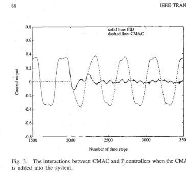
remains constant. The CMAC is added at the sixth cycle, and then the error reduces quickly and significantly. The error remains small for some time, and then it diverges around the 143th cycle. Fig. 3 shows the interactions between the CMAC control U, and the proportional control U, after the CMAC is added: the CMAC quickly learns the inverse mapping of the plant and becomes the dominating controller.
A. Discussion
1) The CMAC can significantly reduce the tracking error. In Fig. 2, the error is 0.252 when solely controlled by the proportional controller (with P = 1.4), which can be reduced to a minimum of 0.018 by the CMAC in a very short time.
2) Despite the promising aspect above, the CMAC can destabilize a control system which is otherwise stable. The unstable phenomenon certainly comes from the interactions between the proportional controller and the CMAC network; more details about this are provided in Section IV. Nonetheless, the proportional controller
88
0.6
IEEE TRANSACTIONS ON CONTROL SYSTEMS TECHNOLOGY, VOL. 4, NO. 1, JANUARY 1996
‘solid line: PJD ’
dashed line: CMAC - C error 0.0193 T, 86 TU ? I 1500 2000 2500 3000 3500 -0.8‘ 0.0209 0.020 0.0199 0.0182 0.0244 0.0198 67 35 15 6 6 6 ? 977 288 143 70 28
Number of time steps
Fig. 3.
is added into the system.
The interactions between CMAC and P controllers when the CMAC
1
...
-2 1
5700 5750 5800 5850 5900 5950 6ooo
Number of time steps
Fig. 4. The system output quickly runs away after the P controller is removed.
can not be removed even when the magnitude of the proportional control is very small compared with that of the CMAC (i.e., when the system output error has been significantly reduced). Otherwise, the good tracking can not be maintained. Fig. 4 shows what happens when the proportional controller is removed at k = 6000: the system output quickly runs away from the desired trajectory and falls into an equilibrium point of the plant. Iv. A SYSTEMATIC STUDY OF THE UNSTABLE PHENOMENON
As is shown in the previous section, the CMAC can signif- icantly improve the performance of existing nonlinear control systems, but the improved performance may only maintain for some period before the CMAC control system goes unstable. In this section, we will again use the CMAC control system in Fig. 1 to quantitatively study how the unstable phenomena is related to such parameters as proportional gain, learning rate, generalization, and quantization. The simulation in this section is the same as that performed in the previous section, except that the system parameters are adjusted in systematic ways to test how they are related to instability. The results are listed in
TABLE I THE EFFECT OF P GAIN
1 g a i n o f P ) 0.6
I
0.81
1.0I
1.21
1.41
1.61
1.81
I P error I 0.5940 I 0.4439 1 0.3540 1 0.2942 I 0.2516 I 0.2198 1 0.1951 1
Tables I-IV. Unless specified otherwise, the parameters used in the simulations are:
learning rate = 0.1
quantization = 51500
generalization = 50
proportional gain = 1.2
reference command = sin ( 2 n k / 4 0 0 ) simulation time = 7500 cycles.
The notations appearing in the tables are:
P error: maximum output error when controlled by the proportional controller only (no CMAC added). C error: the minimum of maximum output error (in a cycle) that can be achieved after the CMAC is added to the control system.
T,: the time (in terms of cycle number, each cycle containing 400 time steps) required for the minimax error to become less than 0.03.
TzL: the time when the output error becomes larger than
“P error.” After that, the output would soon diverge to
infinity.
?: means the system has not diverged when simulation stops at 7500 cycles.
In the following, we discuss the effect of parameters on system stability.
A. Gain of Proportional Controller
In this part, the proportional gain is the only parameter that is adjusted, and the results are summarize in Table I. Some
from Table I are:
The larger the proportional gain is, the smaller the “P error” is.
The most interesting fact is that the “C error” is around 0.02 no matter what the proportional gain is. T, is smaller, however, when the proportional gain is larger. The system can eventually go unstable. The trend is clearly that the system diverges sooner when the propor- tional gain increases. When gain = 0.8 and 0.6, however, the system does not diverge when the simulation ends. Once the simulation was modified to run for ten times longer for these two gains. The system did not diverge, and the tracking error maintains at the level of 0.034. Since it is important to figure out how a system can be destabilized by the CMAC, our discussions in the rest of this section will have the proportional gain fixed at 1.2. When the gain is further reduced (e.g., 0.4 or less), the CMAC cannot effectively improve tracking accuracy. B. Leaming Rate
According to Table 11, the system diverges no matter what the learning rate is. Table 11, however, reveals a very important
IEEE TRANSACTIONS ON CONTROL SYSTEMS TECHNOLOGY, VOL. 4, NO. 1 learning rate p C error T, T,. lANUARY 1996 89 0.5 0.1 0.05
I
0.011
0.0051
0.001 0.0154 0.0199 0.0173 0.0167 0.0161 0.0164 6 15 66 288 I 532 I 2770 5222 , 24482 if T=I
33.5I
28.8I
26.61
27.7I
26.1I
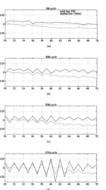
24.5 40th cycle 0.4 I I -0.4L I 0 50 100 150 200 250 300 350 400 Time steps Fig. 5.feature: the product of p and Tu is about a constant, that is, when the learning rate decreases, the time at which the system diverges would increase in proportion.
We explain this feature more clearly in the following: For the several p values tested in Table 11, typically the CMAC would quickly learn the inverse dynamics and the tracking error would decrease rapidly, and then the system gets into a prolonged “stable” period lbefore diverging (see Figs. 2 and 3 for examples). Just very shortly before divergence, the synchronous and quickly increasing oscillations of U, and U, are always observed I[e.g., Fig. 6(d)]. Actually, the wild synchronous oscillations in the last stage do not come all of a sudden. During the prolonged “stable” period, the synchronous oscillations of U, ,and U, can always be detected, and their magnitudes on the average are very slowly but steadily increasing. To demonstrate this, again we look at the case studied in Section 111 as an example. That system diverges at the 143th cycle. Fig. 5 show!; U, and U, for the entire 40th cycle, in which it is notable that there are obvious oscillations around the 50th and 250th time step of that cycle. To show that these oscillations exist and grow in the prolonged “stable” period, we plot U, and U, from the 50th to the 70th time steps for each of the eighth, 40th, 90th and 155th cycles, and these plots are shown in Fig. 6, in which the constant 0.3 is added to U, to make the comparison of U, and U, easier. The reason that pTu is about a constant is obviously that faster learning
in the CMAC would proportionally speed up the appearance
of large in-phase oscillations in U, and U,, which contributes to the instability of the system.
C, Generalization
Table 111 shows the cases with the generalization g ranging from 40 to 200. When g is less than 40, the CMAC cannot
The CMAC and P controls for a complete cycle.
8th cycle
Bolid line: PID ’
dashed line, CMAC
0.05
i
0 -0051 , , , , , , , , ,{
50 52 54 56 58 60 62 64 66 68 70 (a) 40th cycle 0 05 0 -0 05 01
-0 051
50 52 54 56 58 60 62 64 66 68 70 (b) 0.05 0 -0.05 50 52 54 56 58 60 62 64 66 68 70 (C) 155th cycler
I 0 05 0 -0 05 50 52 54 56 58 60 62 64 66 68 70 (4Fig. 6. The growth of oscillations in CMAC and P controls.
effectively learn the inverse dynamics. These important ob- servation from Table I11 is that, when g increases, Tu also increases, and the ratios Tu/g are constants of the same order. Generalization is something indispensable in the application of CMAC to control problems. It enables the CMAC to generate controls based on previous learnings. Generalization, however, can slow down the learning process, in particular when the CMAC is fine-tuning itself for higher precision. Therefore, increasing generalization is almost equivalent to reducing the learning rate p. This explains why Tu increases almost proportionally with g.
D. Quantization
To minimize the effect of generalization on the discussions of quantization, the g in Table IV is varied according to quan- tization, such that about the same overlap can be maintained for different quantizations. It is clear from Table IV that Tu decreases when quantization gets coarser. This is because more
90 gain of P deadzone do C error IEEE TRANSAC 1 0 1 2 1.4 1.6 1.8 0.033 0.04 0.049 0.053 0.063 0.036 0.0312 0.0384 0 0410 0 056 TABLE III
THE EFFECT OF GENERALIZATION generalization g 40 50 60 C error 0.023 0.020 0.017 T S 1 5 1 5 6 TU 183 288 407 Tu/g 4.575 5.76 6.78 100 200 300 0.016 0.0055 0.0047 6 7 9 778 1556 2103 7.78 7.78 7.01 quantization generalization C error T U
noise is introduced into the system when the precision of CMAC degrades. 5/20 5/50 5/200 5/500 5 / S O O 2 5 20 50 80 0.163 0.0687 0.0275 0.0199 0.0168 19 41 190 288 306 E. Discussion
The most important clue about the system instability appears in the discussions concerning learning rate. One may therefore conclude that the continued learning of CMAC after the tracking error has reduced is the major cause of the instability.
v.
METHOD FOR IMPROVING SYSTEM S T A B E l T YBased on the conclusion of the previous section that the continued learning of CMAC after the tracking error has reduced is the major cause of the instability, one may be ready to suggest stopping the CMAC learning after the tracking error is attenuated by the CMAC. Our simulations show that this method can prevent the system from diverging. Stopping the CMAC learning, however, has two drawbacks. First, it can be difficult to determine when to stop the CMAC learning. Second, if the CMAC stops learning, then the CMAC control system cannot respond to any change in the reference command. This is a serious consequence.
To effectively stop the CMAC learning when the tracking error is small, but at the same time allow the system to respond to any change in the reference command, we propose to add a deadzone to the CMAC updating rule. The learning rule described in Section I1 is modified as
where
0 if 1x1
5
doi
z + d o if z<
-doD [ x ] = 2 - d o if z
>
cl0 (4) with do being the deadzone size. The essence of this modified learning rule is not to update the CMAC table if the error is small enough. This modified learning rule is used to rerun the unstable cases of Table I, with the results reported in Table V. In Table V, “deadzone do” means the smallest do required for the system to run for 75 000 cycles without going unstable. Table V shows that, with the addition of a small deadzone, the stability can very significantly be improved without much degrading in tracking precision. For example,TIONS ON CONTROL SYSTEMS TECHNOLOGY, VOL. 4, NO. 1, JANUARY 1996
TABLE V
THE EFFECT OF DEADZONE ON STABILITY
when the proportional gain equals 1.4, the system diverges at the 143rd cycle (see Table I). But the system can run for 75 000 cycles with a deadzone of size 0.049 (the program stops at the 75QWth cycle). This deadzone would cause a degrade in “C error” from 0.0182 to 0.0384, which is not serious at all compared with the error of 0.25 when the CMAC is not used. We conclude this section by saying that deadzone is a very effective method for improving system stability.
VI. EXPERIMENT
The purpose of this section is to control a real world system to show the validity of the simulation results in previous sections.
The system under study is an inverted pendulum driven by a 35 w motor with a gear box, produced by Hi-T Drive. The steel rod is 0.25 m long, with a metal mass of weight 3 kg attached to its end. The motor is driven by UT-SO, a current drive. The sampling interval is 5 ms (i.e., 0.005 s), but the control is calculated and sent to UT-SO only 1 ms after the data are measured. Based on the general discrete-time model of inverted pendulums, the variables B ( k ) , B(k - 1) and
Qd(k
+
1) are selected as the inputs to the CMAC, wheree(
k ) is the actual pendulum angle at time 5 and Bd(k) is the desiredpendulum angle at time k . Other CMAC parameters are: learning rate p, = 0.01, generalization = 100, and quantization
= 3.927/1024. The reference command is a sinusoidal curve, with four seconds in period and *n/5 radian in magnitude. The control software is implemented on a 486 PC. Since the entire CMAC table takes less than 400 kbytes, it is completely implemented and no hash coding is used.
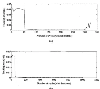
The control results are described in this paragraph. We first tried to control the inverted pendulum by proportional controllers. The proportional controller can not achieve good tracking unless the gain is very large, which is not desirable in practice. The more serious thing is that, the tracking error can only be improved for two to three times at best after the GMAC is added to the system, and the problem is: the proportional controller cannot provide suitable control at the corner where the pendulum is supposed to turn around; as a result, it cannot provide a good example for the CMAC to learn, in the sense that the CMAC learning locations are too far away from the recall locations. This situation is much improved after the proportional controller is replaced by a PD (proportional-differential) controller, with the result shown in Fig. 7(a). The proportional and differential gains used are P = 2037 and D = 611. These gains are very rkasonable from a practical point of view, and they are comparable to the PD gains used in [9] for two-link robotics control problems. Two important messages are provided in Fig. 7(a). First, the tracking error is reduced for about SO times after the CMAC is introduced at the 50th cycle. Second, after 280 cycles,
IEEE TRANSACTIONS ON CONTROL SYSTEMS TECHNOLOGY, VOL. 4, NO. 1, JANUARY 1996 ~ 91 0.05, I
i:.:n
, _ _ _ , , ~1
2 0.02 B5
0.01 0 50 100 150 200 250 300 350Number of cycles(without deazone)
(a) 0 . 0 5 1 I I g 0.01 I 200 400 600 800 lo00 1200 0
-Number of cycles(with deadzone)
(‘b)
Fig. 7. The experimental results without and with deadzone.
the motor becomes very noisy and the system shows large vibrations. Finally we have to shut down the machine. These phenomena match with our observations in simulations.
Next we demonstrate how s8ystem stability is improved by applying deadzone to the CMAC learning rule. The control U ( k ) generated from the computer software is between f 1 2 0 , which is subsequently transformed and scaled by the driving system into actual control torque. The deadzone size used is 20, i.e., there is no updating in the CMAC table when the difference between U and U, ILS less than 20. The stability of
the system is improved as is shown in Fig. 8(b). In practice, the deadzone can be assigned a large value in the initial testing such that the system stability would not be affected immediately. Then, the deadzone can be slowly decreased to appreciate the improvement in tracking provided by the CMAC, until some undesired (effect starts to show up.
A final note about the experiment is that, the PD control results (without CMAC) can be improved if the P and D gains are increased, but the magnitude of PD control would increase as well, and the control would contain large oscillations. In contrast, adding CMAC to the system would not increase the magnitude of the total control, would not cause large oscillations, and can achieve better accuracy than just increase PD gains, as long as suitable measures are taken to prevent the system from diverging, for example, using a deadzone.
VII. CONCLUSION
The main points of this paper are summarized as follows:
1) The CMAC can be a powerful and low-cost tool to im-
prove existing nonlinear control systems. It is powerful
because it can very quickly learn the inverse mapping of the plant and generate precise controls. It is low-cost because it can be easily implemented and added onto the original control system without much modification to the original control designs.
The CMAC control system can potentially go unstable. The problem is more with the control scheme than with the CMAC itself. The CMAC controller and the traditional controller (e.g., the PID) are independent of each other, and the actual control to the plant is the sum of these two controllers. During the initial stage, a transition in control from PID to CMAC is observed and precise tracking is quickly achieved. After lengthy and complex interactions between the PID and the CMAC, however, the in-phase wild oscillations of these two controllers destabilize the system. We propose to use deadzone as an effective tool to stop the formation of large oscillations, to maintain the good tracking contributed by the CMAC.
Since the role of the neural network in this control system is to learn the inverse mapping of the plant, any other neural networks capable of doing this can be used in the place of the CMAC, for example, the backpropagation networks or the Gaussian networks.
Although we propose to use deadzone to improve system stability, this may not be the only way stability can be improved. An interesting thing to see in the future would be to apply the CMAC to complex systems, and do quantitative study on issues about efficiency and stability.
REFERENCES
J. S . Albus, “Data storage in the cerebellar model articulation controller,” J. Dynamic Syst., Measurement, Contr., pp. 228-233, Sep. 1975. -, “A new approach to manipulator control: The cerebellar model articulation controller (CMAC),” J. Dvnamic Svst., Measurement, Contr.. pp. 220-227, Sep. 1975.
W. T. Miller, F. H. Glanz, and L. G. Kraft, “Application of a general learning algorithm to the control of robotics manipulators,” Int. J.Robot.
Res., vol. 6, pp. 84-98, Summer 1987.
W. T. Miller, R. H. Hewes, F. H. Glanz, and L. G. Kraft, “Real-time
dynamic control of an industrial manipulator using a neural-network- based learning controller,” ZEEE Trans. Robot. Automat., vol. 6, no. 1, pp. 1-9, Feb. 1990.
Y. Wong and A. Sideris, “Learning convergence in the cerebellar model
articulation controller,” ZEEE Trans. Neural Networks, vol. 3 , no. 1, pp. 115-122, Jan. 1992.
S. H. Lane, D. A. Handelman, and J. J. Gelfand, “Theory and develop- ment of higher-order CMAC neural networks,” ZEEE Contr. Syst. Mug., pp. 23-30, Apr. 1992.
C.-S. Lin and H. Kim, “CMAC-based adaptive critic self-learning control,” ZEEE Trans. Neural Networks, vol. 2, no. 5 , pp. 530-533,
Sep. 1991.
W. T. Miller, 111, “Real-time neural network control of a biped walking robot,” ZEEE Contr. Syst. Mag., vol. 14, no. 1, pp. 4 1 4 8 , Feb. 1994. J.-J. E. Slotine and W. Li, Applied Nonlinear Control. Englewood Cliffs, NJ: Prentice-Hall, 1991.