Non-Coherent Cell Identification Detection Methods
and Statistical Analysis for OFDM Systems
Chih-Liang Chen and Sau-Gee Chen
Abstract—To achieve high-performance cell identification de-tection with low complexity for orthogonal frequency division multiplexing (OFDM) systems, this work proposes an efficient non-coherent cell identification (ID) detection technique based on a new optimization metric. Furthermore, the metric is simplified to two lower-complexity metrics. As such, two more modified cell ID detection methods extended from the first one are also proposed. Experiments show that all the three new cell ID methods achieve better performances than the conventional methods in multipath Rayleigh fading channels. This work also conducts the statistical analysis to characterize the proposed techniques completely. It is shown that the results of the theoretical analysis are close to the simulation results. Among the new techniques, specifically, the third proposed method using the second simplified new metric has much lower complexity and higher performance than the conventional methods.
Index Terms—Orthogonal frequency division multiplexing (OFDM), cell identification, cell identification detection, multi-path fading channel.
I. INTRODUCTION
S
INCE the recent decade, the demand for portable deviceswith wireless real-time and high-rate multimedia services has been in a rapid growing pace. To meet the demand, the cellular orthogonal frequency division multiplexing (OFDM) system is widely adopted by many current and next-generation wireless communication specifications, including the IEEE 802.16e, 802.16m and 3GPP LTE systems. In a cellular OFDM system, a serial data stream is split into several parallel data streams. Then, each parallel data stream modulates its corresponding subcarrier which is orthogonal to all the other subcarriers. Thus, for each subcarrier, OFDM technique trans-forms the frequency-selective fading channel into many flat-fading subchannels. This feature significantly simplifies the equalizer designs. Besides, by adding a cyclic prefix (CP) to the beginning of each OFDM symbol, the intersymbol interference (ISI) caused by the channel delay spread can be reduced and the subcarrier orthogonality can be maintained.
When a mobile station (MS) wants to access a cellular OFDM system, it needs to know the cell identification (ID) information of the cell it resides. In most existing systems (for example, IEEE 802.16e/j), non-hierarchical preamble struc-tures [2][3] with a large number of cell-specific sequences are
Paper approved by E. Perrins, the Editor for Modulation Theory of the IEEE Communications Society. Manuscript received August 12, 2009; revised April 19, 2010 and June 19, 2010.
Parts of this work have been presented at the IEEE Personal, Indoor and Mobile Radio Communications (PIMRC) Conference, 2008.
The authors are with the Department of Electronics Engineer-ing and Institute of Electronics, National Chiao Tung University, 1001 University Road, Hsinchu, Taiwan (e-mail: [email protected]; [email protected]).
Digital Object Identifier 10.1109/TCOMM.2010.091710.090472
adopted. In this work, we also assume the non-hierarchical structure. To obtain the cell ID involves complicated and computational intensive matching operations. Hence, for the consideration of low access delay and low complexity, a highly efficient and accurate cell ID detection process is required to find out the index of the transmitted preamble.
There are two kinds of cell ID detection methods, namely coherent and non-coherent methods, for cellular OFDM sys-tems in the literature. Coherent cell ID detection methods [3][4][5][6] require channel information, while non-coherent cell ID detection methods [7][8][9][10][11] do not. For practi-cal systems, normally initial synchronization processes includ-ing the cell identification are conducted first, followed by the process of channel estimation. That is, non-coherent methods are mostly adopted by current communication systems. As such, this work assumes non-coherent cell ID detection and focuses on improving the performances of the non-coherent cell ID detection methods. For IEEE 802.16e OFDM system [13][14], the cell ID detection method [7] is based on an autocorrelation technique. The autocorrelation technique de-termines the cell ID by detecting the maximum value of all the correlation values between the received frequency-domain signal and all the reference preamble signals. In [22], authors propose two frame detection methods (namely TD and FD) and combine those methods with adaptive correlation length (ACL). With shorter correlation length, [22] can reduce the computational complexity during the cell ID identification stage. However, note that [22] still utilizes the conventional correlation procedure during the cell ID identification stage. Thus, it is a simplified autocorrelation method.
However, in multipath fading channel environments, the frequency-domain correlation is likely influenced by frequency selective fading. As such, differential demodulation is em-ployed prior to the autocorrelation for mitigating the frequency selective fading. In fact, most of the existing non-coherent cell ID methods [8][9][10][11] for cellular OFDM systems are based on the differential autocorrelation technique. Hence, this work will directly compare the performance and complexity between the proposed methods and the differential autocor-relation technique. Although the differential autocorautocor-relation technique has high performance, the most critical disadvantage of the differential autocorrelation technique is that it requires a large number of complex multiplication operations. For exam-ple, since there are 114 sets of known reference preambles in IEEE 802.16 and IEEE 802.16e OFDM systems, the involved computation complexity is enormous for those autocorrelation-based methods. Beside, a technique in [21], called the code group identification method, detects the code group ID by dividing the received signal into four non-overlapping parts.
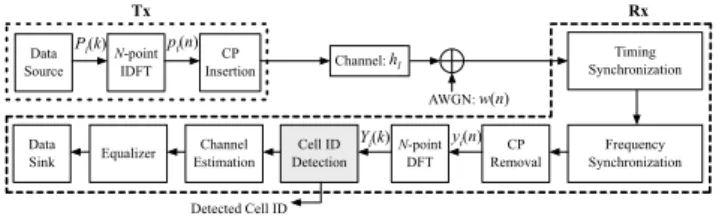
Data Source N-point IDFT CP Insertion Channel: CP Removal N-point DFT Channel Estimation Equalizer Data Sink Frequency Synchronization Cell ID Detection Timing Synchronization AWGN: Tx Rx Pi(k) pi(n) hl w(n) yi(n) Yi(k) Detected Cell ID
Fig. 1. Simplified discrete-time OFDM system structure.
The method will achieve good integration gain if the channel variation is small or the channel response is flat, otherwise the integration gain will be low if the channel variation is large or the channel response is highly frequency selective. Therefore, in that case, it will misdetect the preamble sequence.
To significantly reduce the complexity and achieve high performance at the same time, this paper proposes three efficient non-coherent cell ID detection methods based on a new optimization metric and its simplifications. These new methods are not only suitable for IEEE 802.16 and IEEE 802.16e systems but also suitable for other preamble-based OFDM systems. By combining a preamble matching process and a multiplication-free smoothing scheme, the proposed techniques achieve better performances than the existing tech-niques in multipath Rayleigh fading channels. Based on our preliminary work [1], which introduces a basic concept of smoothing for cell ID detection, this paper generalizes the design concept and provide a statistical characterization for the proposed methods. Moreover, for further reducing the
complexity, we introduce the decimation factor 𝑑 into the
conventional and proposed methods as shown in the section of simulation results. With the decimation, all the methods can achieve lower computational complexities. For a sys-tem suffering the burst error, reducing the complexity by decimation may be better than reducing the complexity by directly shortening the correlation length in [22]. Therefore,
by appropriately choosing the value of decimation factor 𝑑,
the proposed methods can achieve the similar complexities as [22], but with better system performances.
The rest of this paper is organized as follows. Section II describes the OFDM system model and the differential au-tocorrelation technique adopted by conventional cell ID de-tection methods. Section III introduces the proposed cell ID detection methods based on three new optimization metrics. In Section IV, theoretical analysis of the proposed optimization metric is conducted which includes the mean value analysis and the lower bound analysis of the variance. Section V provides the computational complexity analysis of the con-ventional and the proposed methods. Simulation results in different channel conditions are presented in Section VI. Finally, Section VII is the conclusion.
II. OFDM SYSTEMMODEL ANDCONVENTIONAL
DIFFERENTIALAUTOCORRELATIONTECHNIQUE A. OFDM System Model
Fig. 1 shows a simplified discrete-time OFDM system
structure, where𝑁 is the total number of subcarriers. For cell
identification, it is assumed that the system is transmitting a
specific preamble signal 𝑃𝑖(𝑘), 0 ≤ 𝑘 ≤ 𝑁 − 1, where 𝑖
and 𝑘 are the preamble index and subcarrier index,
respec-tively. This work assumes that the transmitted preamble is BPSK-modulated pseudo-noise (PN) code (as defined in IEEE 802.16e standard) and the total number of the known reference
preambles is𝑀. In the cell ID detection process, 𝑃𝑖(𝑘) is to be
identified from the set of all the possible reference preambles
𝑃𝑚(𝑘), 0 ≤ 𝑚 ≤ 𝑀 − 1. The modulators in the transmitter
and the matched filters in the receiver for the OFDM systems can be implemented by IDFT and DFT [12], respectively. The signal after IDFT is
𝑝𝑖(𝑛) = 𝑁1
𝑁−1∑ 𝑘=0
𝑃𝑖(𝑘)𝑒𝑗2𝜋𝑘𝑛𝑁 , 0 ≤ 𝑛 ≤ 𝑁 − 1. (1)
The signal is then preceded with a CP and delivered through a time-invariant Rayleigh fading channel. The channel paths
ℎ𝑙, 0 ≤ 𝑙 ≤ 𝐿 − 1, are assumed uncorrelated zero-mean
complex Gaussian random variables with variance𝜎2
ℎ𝑙, where
𝐿 is the total number of channel paths. After the timing
synchronization and frequency synchronization, the timing and frequency offset can be compensated. Therefore, the received signal can be represented as
𝑦(𝑛) =
𝐿−1∑ 𝑙=0
ℎ𝑙𝑝𝑖(𝑛 − 𝑙)𝑁 + 𝑤(𝑛), (2)
where (⋅)𝑁 represents the modulo 𝑁 operation and 𝑤(𝑛) is
a zero-mean additive white complex Gaussian noise (AWGN)
with variance 𝜎2
𝑤. The received signal after DFT at the𝑘-th
subcarrier is
𝑌 (𝑘) =𝑁−1∑
𝑛=0
𝑦(𝑛)𝑒−𝑗2𝜋𝑘𝑛
𝑁 . (3)
By substituting (1) and (2) into (3), the 𝑘-th subcarrier
signal𝑌 (𝑘) is
𝑌 (𝑘) = 𝐻(𝑘)𝑃𝑖(𝑘) + 𝑊 (𝑘), (4)
where 𝐻(𝑘) is the channel frequency response at the 𝑘-th
subcarrier, namely,
𝐻(𝑘) =𝐿−1∑
𝑙=0
ℎ𝑙𝑒−𝑗2𝜋𝑙𝑘𝑁 , 0 ≤ 𝑘 ≤ 𝑁 − 1,
and𝑊 (𝑘) is the DFT of the zero-mean AWGN 𝑤(𝑛), i.e., 𝑊 (𝑘) =
𝑁−1∑ 𝑛=0
𝑤(𝑛)𝑒−𝑗2𝜋𝑘𝑛𝑁 , 0 ≤ 𝑘 ≤ 𝑁 − 1.
Note that since the channel paths ℎ𝑙 and AWGN 𝑤(𝑛) are
complex Gaussian random variables,𝐻(𝑘) and 𝑊 (𝑘) are also
complex Gaussian random variables.
Although timing synchronization and frequency synchro-nization are performed before the cell ID identification stage,
residual timing error 𝜏 and residual frequency offset 𝜖 may
still exist. As such, for a complete system modeling, (4) can be further revised [19][20] as 𝑌 (𝑘) = 𝐻(𝑘)𝑃𝑖(𝑘)𝐿(𝑘) + 𝐼(𝑘) + 𝑊 (𝑘)𝑒𝑗−2𝜋𝑘𝜏𝑁 , (5) where 𝐿(𝑘) ≡ 𝑁 sin(sin(𝜋𝜖)𝜋𝜖 𝑁) 𝑒𝑗𝜋(𝑁𝜖−𝜖−2𝑘𝜏) 𝑁 ,
and 𝐼(𝑘) is inter-carrier interference (ICI) caused by the
frequency offset and represented as
𝐼(𝑘) ≡∑𝑁−1𝑚=0,𝑚∕=𝑘𝐻(𝑚)𝑃𝑖(𝑚) ×𝑁 sin(sin(𝜋(𝜖+𝑘−𝑚))𝜋(𝜖+𝑘−𝑚)
𝑁 )
× 𝑒𝑗𝜋(𝜖+𝑘−𝑚)(𝑁−1)𝑁 𝑒𝑗−2𝜋𝑘𝜏𝑁 .
Note that the channel paths and AWGN are complex Gaussian random variables, and are also complex Gaussian random vari-ables. The next step is to recognize the transmitted preamble index (i.e., cell ID) from all the possible preambles.
B. Conventional Differential Autocorrelation Technique
Basically, the conventional differential autocorrelation tech-nique [8][9][10][11] can be represented as
ˆ𝑖 = arg max 0≤𝑚≤𝑀−1 𝑁−2∑ 𝑘=0 𝑌 (𝑘)𝑌∗(𝑘 + 1)𝑃 𝑚(𝑘)𝑃𝑚(𝑘 + 1), (6)
where ˆ𝑖 is the detected cell ID. For explaining the idea
of the conventional technique, the discussion starts with the
following preamble matching operation at the𝑘-th subcarrier:
𝑀𝑖,𝑚(𝑘) = 𝑌 (𝑘)𝑃𝑚(𝑘) = 𝐻(𝑘)𝑃𝑖(𝑘)𝑃𝑚(𝑘)𝐿(𝑘) + 𝐼(𝑘)𝑃𝑚(𝑘) + 𝑊 (𝑘)𝑃𝑚(𝑘)𝑒𝑗−2𝜋𝑘𝜏𝑁 = 𝐻(𝑘)𝑋𝑖,𝑚(𝑘)𝐿(𝑘) + 𝐼(𝑘)𝑃𝑚(𝑘) + 𝑊 (𝑘)𝑃𝑚(𝑘)𝑒𝑗−2𝜋𝑘𝜏𝑁 , (7) where 𝑋𝑖,𝑚(𝑘) ≡ 𝑃𝑖(𝑘)𝑃𝑚(𝑘).
Because of the BPSK-modulated preambles, there are only
two possible outcomes of𝑋𝑖,𝑚(𝑘) as shown below
𝑋𝑖,𝑚(𝑘) =
{
1, if 𝑖 = 𝑚
±1, if 𝑖 ∕= 𝑚. (8)
Further, with (7), the correlation term 𝑀𝑖,𝑚(𝑘)𝑀𝑖,𝑚∗ (𝑘 + 1)
is 𝑀𝑖,𝑚(𝑘)𝑀𝑖,𝑚∗ (𝑘 + 1) = 𝐻(𝑘)𝐻∗(𝑘+1) × 𝑋𝑖,𝑚(𝑘)𝑋𝑖,𝑚∗ (𝑘+1) × (𝑁 sin(sin(𝜋𝜖)𝜋𝜖 𝑁)) 2𝑒𝑗2𝜋𝜏 𝑁 + ¯𝑊, (9) where𝑀∗
𝑖,𝑚(𝑘 + 1) is the complex conjugate of 𝑀𝑖,𝑚(𝑘 + 1)
and ¯ 𝑊 = 𝐻(𝑘)𝑋𝑖,𝑚(𝑘)𝐿(𝑘) ×[𝐼∗(𝑘 + 1)𝑃 𝑚(𝑘 + 1) + 𝑊∗(𝑘 + 1)𝑃𝑚(𝑘 + 1)𝑒𝑗2𝜋𝑘𝜏𝑁 ] +𝐼(𝑘)𝑃𝑚(𝑘) × [𝐻∗(𝑘 + 1)𝑋𝑖,𝑚(𝑘 + 1)𝐿∗(𝑘 + 1) +𝑊∗(𝑘 + 1)𝑃 𝑚(𝑘 + 1)𝑒𝑗2𝜋𝑘𝜏𝑁 ] +𝑊 (𝑘)𝑃𝑚(𝑘)𝑒𝑗−2𝜋𝑘𝜏𝑁 ×[𝐻∗(𝑘 + 1)𝑋 𝑖,𝑚(𝑘 + 1)𝐿∗(𝑘 + 1) +𝐼∗(𝑘 + 1)𝑃 𝑚(𝑘 + 1)] +𝐼(𝑘)𝑃𝑚(𝑘)𝐼∗(𝑘 + 1)𝑃𝑚(𝑘 + 1) +𝑊 (𝑘)𝑃𝑚(𝑘)𝑊∗(𝑘 + 1)𝑃𝑚(𝑘 + 1) (10)
With (8), by ignoring the noise term ¯𝑊 and assuming similar
frequency responses at the neighbor subcarriers (i.e.,𝐻(𝑘) ≈
𝐻(𝑘 + 1)), (9) can be reduced to 𝑀𝑖,𝑚(𝑘)𝑀𝑖,𝑚∗ (𝑘 + 1) ≈ ⎧ ⎨ ⎩ ∣𝐻(𝑘)∣2× ( sin(𝜋𝜖) 𝑁 sin(𝜋𝜖 𝑁)) 2𝑒𝑗2𝜋𝜏 𝑁 , when 𝑖 = 𝑚 ±∣𝐻(𝑘)∣2× ( sin(𝜋𝜖) 𝑁 sin(𝜋𝜖 𝑁)) 2𝑒𝑗2𝜋𝜏 𝑁 , when 𝑖 ∕= 𝑚 (11)
where∣(.)∣ is the absolute-value operation.
Basically, with (11), the differential autocorrelation tech-nique of the conventional cell ID detection methods identifies
cell preamble index𝑖 by detecting the maximum value of the
following correlation metric [8][9][10][11] . ˆ𝑖 = arg max
0≤𝑚≤𝑀−1
𝑁−2∑ 𝑘=0
𝑀𝑖,𝑚(𝑘)𝑀𝑖,𝑚∗ (𝑘 + 1). (12)
Note that (12) is equivalent to (6).
Since the result of the differential autocorrelation
∑𝑁−2
𝑘=0 𝑀𝑖,𝑚(𝑘)𝑀𝑖,𝑚∗ (𝑘 + 1) is generally a complex number
in practical situations, the maximum-value search process (i.e.,
𝑎𝑟𝑔𝑚𝑎𝑥) should compare the magnitude of the differential
autocorrelation. As such, the conventional differential auto-correlation method should be
ˆ𝑖 = arg max
0≤𝑚≤𝑀−1∣
𝑁−2∑ 𝑘=0
𝑀𝑖,𝑚(𝑘)𝑀𝑖,𝑚∗ (𝑘 + 1)∣. (13)
Moreover, with the obtaining the magnitude, the effects of the residual frequency offset and the residual timing error can be eliminated as well. However, it would involve high-complexity square-root operations in obtaining the magnitude of the differential autocorrelation. For reducing the complexity, the absolute-value operations can be replaced with the squared absolute-value operations. Each squared absolute-value oper-ation only involves two real-number square operoper-ations and a real-number addition operation. Hence, (13) can be adjusted to ˆ𝑖 = arg max 0≤𝑚≤𝑀−1∣ 𝑁−2∑ 𝑘=0 𝑀𝑖,𝑚(𝑘)𝑀𝑖,𝑚∗ (𝑘 + 1)∣2. (14)
For further complexity reduction, this work will simplify the absolute-value operations in (13) by adopting another approach, which will be presented in Section V. Besides, Section V will also compare the conventional methods in all the mentioned forms (i.e., (13), (14), and (45) in Section V) with the proposed methods.
III. PROPOSEDCELLID DETECTIONMETHODS
The mentioned conventional cell ID detection methods are subject to noise interference and frequency-selective channel
effect (when the assumption of𝐻(𝑘) ≈ 𝐻(𝑘 + 1) frequently
fails), which lead to performance degradation. In order to enhance the performances of cell ID detection and reduce the complexities, this work proposes the following channel-effect-resilient cell ID detection method (CERCD-I) to mitigate the effects of AWGN and fading channels,
ˆ𝑖𝐼 = arg max
0≤𝑚≤𝑀−1
𝑁−𝑅∑ 𝑘=0
−5 −4 −3 −2 −1 0 1 2 3
10−2
10−1
100
SNR(dB)
Probability of the Incorrect Detection
R=2 R=3 R=4 R=5 R=6
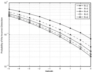
Fig. 2. The probability of the incorrect cell ID detection in a 6-path Rayleigh fading channel of the ITU-R vehicular A channel model.
based on a new optimization metric𝑆𝑖,𝑚(𝑘) defined below
𝑆𝑖,𝑚(𝑘) ≡
𝑅−1∑ 𝑟=0
𝑎𝑟× 𝑀𝑖,𝑚(𝑘 + 𝑟), (16)
where 𝑎𝑟 is the signal smoothing coefficient, and 𝑅 is the
number of the smoothed𝑀𝑖,𝑚(𝑘) terms.
For determining parameter 𝑅, one can first consider the
features of the optimization metric 𝑆𝑖,𝑚(𝑘). Since the
pro-posed method utilizes the concept of the signal filtering in
𝑆𝑖,𝑚(𝑘), one can expect that better performance will be
achieved by taking more 𝑀𝑖,𝑚(𝑘) terms into consideration.
As such, as shown in Fig. 2, a higher 𝑅 leads to a better
system performance. However, a lager 𝑅 corresponds to a
higher computational complexity than a smaller 𝑅. Besides,
the ID detection performance will be decreased, when𝑅 is
increased to some large value and beyond, even when there is a match in the preamble sequence. It is because that for channels
with high frequency response variations, a large enough𝑅 will
produce a small average gain over the covered𝑅 subcarrier
channel frequency responses. Therefore, the selection of𝑅 is
channel dependent and generally a larger𝑅 performs better
than a smaller𝑅 in some limited range of 𝑅 values. According
to our simulation, the performance is proportional to 𝑅 but
saturates at about𝑅 = 5. However, for the consideration of
low-complexity realization, we choose𝑅 = 3 which provides
better performances than conventional methods and achieves low computational complexities in the meantime.
Regarding the weighting parameter 𝑎𝑟 on 𝑀𝑖,𝑚(𝑘), since
we are assuming non-coherent ID detection and dealing with random channels, statistically all the subcarriers are equally important. Therefore, intuitively the performance of
optimiza-tion metric 𝑆𝑖,𝑚(𝑘) with equal 𝑎𝑟 weight on each 𝑀𝑖,𝑚(𝑘)
will outperform the performance of𝑆𝑖,𝑚(𝑘) with unequal 𝑎𝑟s,
as verified and shown in Fig. 3. In Fig. 3, different𝑎𝑟sets are
assumed to have the same power for a fair comparison (i.e.,
∑𝑅−1
𝑟=0 𝑎2𝑟are the same for all the compared𝑎𝑟sets). Also𝑎𝑟
should better be some trivial numbers for a low-complexity
realization. Therefore, all 𝑎𝑟s are equal to one and it is a
good choice for noise smoothing operation. According to the
−5 −4 −3 −2 −1 0 1 2 3
10−2
10−1
100
SNR(dB)
Probability of the Incorrect Detection
a
r=[1,1,1]
ar=[0.7746,1.0954,1.3416]
ar=[1.0954,1.3416,0.7746]
ar=[1.3416,0.7746,1.0954]
Fig. 3. The probability of the incorrect cell ID detection in a 6-path Rayleigh fading channel of the ITU-R vehicular A channel model.
above reasons, we set𝑅 = 3 and 𝑎𝑟= 1 in the discussion for
the demonstration of the proposed concept.
As such, the proposed metric𝑆𝑖,𝑚(𝑘) is
𝑆𝑖,𝑚(𝑘) = 𝑀𝑖,𝑚(𝑘) + 𝑀𝑖,𝑚(𝑘 + 1) + 𝑀𝑖,𝑚(𝑘 + 2). (17)
Clearly, in (17), there only needs two complex additions in contrast to the complex multiplication in (11) required by con-ventional techniques. As will be shown later, by applying this metric to determine the cell ID, much higher performance and lower computational complexity can be achieved compared with conventional techniques.
Next, we will briefly discuss the concept of the proposed
metric. By substituting (7) into (17),𝑆𝑖,𝑚(𝑘) can be rewritten
as 𝑆𝑖,𝑚(𝑘) = 𝐻(𝑘)𝑋𝑖,𝑚(𝑘)𝐿(𝑘) + 𝐻(𝑘 + 1)𝑋𝑖,𝑚(𝑘 + 1)𝐿(𝑘 + 1) + 𝐻(𝑘 + 2)𝑋𝑖,𝑚(𝑘 + 2)𝐿(𝑘 + 2)+𝑒𝐼+𝑒𝑤, (18) where 𝑒𝐼 ≡ 𝐼(𝑘)𝑃𝑚(𝑘) + 𝐼(𝑘 + 1)𝑃𝑚(𝑘 + 1) + 𝐼(𝑘 + 2)𝑃𝑚(𝑘 + 2) and 𝑒𝑤 ≡ 𝑊 (𝑘)𝑃𝑚(𝑘)𝑒𝑗−2𝜋𝑘𝜏𝑁 + 𝑊 (𝑘 + 1)𝑃𝑚(𝑘 + 1)𝑒𝑗−2𝜋(𝑘+1)𝜏𝑁 + 𝑊 (𝑘 + 2)𝑃𝑚(𝑘 + 2)𝑒𝑗−2𝜋(𝑘+2)𝜏𝑁 .
Note that 𝐻(𝑘) and 𝑊 (𝑘) terms are approximately assumed
substitut-ing𝐼(𝑘) into 𝑒𝐼, the𝑒𝐼 can be further expressed as 𝑒𝐼 ≡ 𝐼(𝑘)𝑃𝑚(𝑘) + 𝐼(𝑘 + 1)𝑃𝑚(𝑘 + 1) + 𝐼(𝑘 + 2)𝑃𝑚(𝑘 + 2) =∑𝑁−1𝑚=0,𝑚∕=𝑘𝐻(𝑚)𝑃𝑖(𝑚)𝑃𝑚(𝑘) ×𝑁 sin(sin(𝜋(𝜖+𝑘−𝑚))𝜋(𝜖+𝑘−𝑚) 𝑁 )𝑒 𝑗𝜋(𝜖+𝑘−𝑚)(𝑁−1) 𝑁 𝑒𝑗−2𝜋𝑘𝜏𝑁 +∑𝑁−1𝑚=0,𝑚∕=𝑘+1𝐻(𝑚)𝑃𝑖(𝑚)𝑃𝑚(𝑘 + 1) × sin(𝜋(𝜖+𝑘+1−𝑚)) 𝑁 sin(𝜋(𝜖+𝑘+1−𝑚)𝑁 )𝑒 𝑗𝜋(𝜖+𝑘+1−𝑚)(𝑁−1) 𝑁 𝑒𝑗−2𝜋(𝑘+1)𝜏𝑁 +∑𝑁−1𝑚=0,𝑚∕=𝑘+2𝐻(𝑚)𝑃𝑖(𝑚)𝑃𝑚(𝑘 + 2) ×𝑁 sin(sin(𝜋(𝜖+𝑘+2−𝑚))𝜋(𝜖+𝑘+2−𝑚) 𝑁 )𝑒 𝑗𝜋(𝜖+𝑘+2−𝑚)(𝑁−1) 𝑁 𝑒𝑗−2𝜋(𝑘+2)𝜏𝑁 (19) According to (19), 𝑃𝑖(𝑚)𝑃𝑚(𝑘), 𝑃𝑖(𝑚)𝑃𝑚(𝑘 + 1), and
𝑃𝑖(𝑚)𝑃𝑚(𝑘 + 2) lead to the randomness of 𝑒𝐼.
With (18),∣𝑆𝑖,𝑚(𝑘)∣ can be further expanded as
∣𝑆𝑖,𝑚(𝑘)∣ = √ 𝐴(𝑘) + 𝐵𝑖,𝑚(𝑘) + 𝐶𝑖,𝑚(𝑘) + 𝐷𝑖,𝑚(𝑘), (20) where 𝐴(𝑘) ≡ (𝑁 sin(sin(𝜋𝜖)𝜋𝜖 𝑁) )2×(∣𝐻(𝑘)∣2+∣𝐻(𝑘 + 1)∣2+∣𝐻(𝑘 + 2)∣2), 𝐵𝑖,𝑚(𝑘) ≡ 𝐻(𝑘)𝑋𝑖,𝑚(𝑘)𝐿(𝑘)𝑒∗𝑤 +𝐻(𝑘 + 1)𝑋𝑖,𝑚(𝑘 + 1)𝐿(𝑘 + 1)𝑒∗𝑤 +𝐻(𝑘 + 2)𝑋𝑖,𝑚(𝑘 + 2)𝐿(𝑘 + 2)𝑒∗𝑤 +𝐻∗(𝑘)𝑋∗ 𝑖,𝑚(𝑘)𝐿∗(𝑘)𝑒𝑤 +𝐻∗(𝑘 + 1)𝑋∗ 𝑖,𝑚(𝑘 + 1)𝐿∗(𝑘 + 1)𝑒𝑤 +𝐻∗(𝑘 + 2)𝑋∗ 𝑖,𝑚(𝑘 + 2)𝐿∗(𝑘 + 2)𝑒𝑤 +𝑒𝐼𝑒∗𝑤+ 𝑒∗𝐼𝑒𝑤+ ∣𝑒𝑤∣2, 𝐶𝑖,𝑚(𝑘) ≡ 𝐻(𝑘)𝑋𝑖,𝑚(𝑘)𝐿(𝑘)𝑒∗𝐼 +𝐻(𝑘 + 1)𝑋𝑖,𝑚(𝑘 + 1)𝐿(𝑘 + 1)𝑒∗𝐼 +𝐻(𝑘 + 2)𝑋𝑖,𝑚(𝑘 + 2)𝐿(𝑘 + 2)𝑒∗𝐼 +𝐻∗(𝑘)𝑋∗ 𝑖,𝑚(𝑘)𝐿∗(𝑘)𝑒𝐼 +𝐻∗(𝑘 + 1)𝑋∗ 𝑖,𝑚(𝑘 + 1)𝐿∗(𝑘 + 1)𝑒𝐼 +𝐻∗(𝑘 + 2)𝑋∗ 𝑖,𝑚(𝑘 + 2)𝐿∗(𝑘 + 2)𝑒𝐼 +∣𝑒𝐼∣2, and 𝐷𝑖,𝑚(𝑘) ≡ 𝐼𝑖,𝑚1(𝑘) × (𝑁 sin(sin(𝜋𝜖)𝜋𝜖 𝑁) )2 ×[𝐻(𝑘)𝐻∗(𝑘 + 1)𝑒𝑗2𝜋𝜏 𝑁 +𝐻∗(𝑘)𝐻(𝑘 + 1)𝑒𝑗−2𝜋𝜏𝑁 ] + 𝐼𝑖,𝑚2(𝑘) × (𝑁 sin(sin(𝜋𝜖)𝜋𝜖 𝑁) )2 ×[𝐻(𝑘)𝐻∗(𝑘 + 2)𝑒𝑗4𝜋𝜏 𝑁 +𝐻∗(𝑘)𝐻(𝑘 + 2)𝑒𝑗−4𝜋𝜏𝑁 ] + 𝐼𝑖,𝑚3(𝑘) × (𝑁 sin(sin(𝜋𝜖)𝜋𝜖 𝑁)) 2 ×[𝐻(𝑘+1)𝐻∗(𝑘+2)𝑒𝑗2𝜋𝜏𝑁 + 𝐻∗(𝑘+1)𝐻(𝑘+2)𝑒𝑗−2𝜋𝜏 𝑁 ], and ⎧ ⎨ ⎩ 𝐼𝑖,𝑚1(𝑘) ≡ 𝑋𝑖,𝑚(𝑘)𝑋𝑖,𝑚(𝑘 + 1) 𝐼𝑖,𝑚2(𝑘) ≡ 𝑋𝑖,𝑚(𝑘)𝑋𝑖,𝑚(𝑘 + 2) 𝐼𝑖,𝑚3(𝑘) ≡ 𝑋𝑖,𝑚(𝑘 + 1)𝑋𝑖,𝑚(𝑘 + 2).
As shown, ∣𝑆𝑖,𝑚(𝑘)∣ consists of four parts. The first part,
𝐴(𝑘), contains the channel power terms and the second part,
𝐵𝑖,𝑚(𝑘), contains the multiplication terms of AWGN, channel
responses and preamble signals. Then, 𝐶𝑖,𝑚(𝑘) contains the
multiplication terms of ICI, channel responses and preamble
signals. Finally, the fourth part,𝐷𝑖,𝑚(𝑘), consists of
multipli-cation terms of the preamble signals and subcarrier responses.
Note that 𝐴(𝑘) is independent of the preamble index 𝑚.
On the other hand, 𝐵𝑖,𝑚(𝑘) and 𝐶𝑖,𝑚(𝑘) corresponds to
noise smoothing and lowpass filtering operations which lead to significantly attenuated results, due to the randomness of
𝐵𝑖,𝑚(𝑘) and 𝐶𝑖,𝑚(𝑘) caused by the AWGN components and
𝑒𝐼, respectively. Hence, 𝐵𝑖,𝑚(𝑘) and 𝐶𝑖,𝑚(𝑘) are generally
small and insignificant in (20) for all 𝑚 values. Finally,
𝐷𝑖,𝑚(𝑘) plays the most dominant role in (20), because the
𝐼𝑖,𝑚(𝑘) terms represent the preamble matching values of
𝑋𝑖,𝑚(𝑘), 𝑋𝑖,𝑚(𝑘 + 1) and 𝑋𝑖,𝑚(𝑘 + 2). If 𝑚 = 𝑖, the
accumulated ∣𝑆𝑖,𝑚(𝑘)∣ will statistically generate a maximum
value among all the possible 𝑚 values. Thus, with (15), the
cell ID with the maximum accumulated magnitude of the proposed metrics, among all the accumulated magnitudes, will be the detected.
Further, it should be also noted that the proposed methods can be generalized to flexibly detect the cell ID by dividing the input into either overlapping or non-overlapping summation segments, subject to cost-and-performance tradeoff. As such, the proposed methods can be generalized to include the method in [21]. The code group identification method in [21] can be derived from the proposed CERCD-I method
by setting the parameters of CERCD-I to 𝑅 = 64 and
𝑎𝑟 = 1 and adjusting the values of accumulation index 𝑘
to 𝑘 = {0, 64, 128, 192}. Since the amount (i.e., 193, 𝑘 = {0, 1, ..., 192}) of accumulated ∣𝑆𝑖,𝑚(𝑘)∣ terms for the
CERCD-I method is much larger than that (i.e., 4, 𝑘 =
{0, 64, 128, 192}) for the method in [21], performance of
the proposed method will be better than the method in [21], in terms of robustness to fading channels . Regarding complexity comparison, owing to the difference in the accumulation terms, the method in [21] has a lower complexity than the CERCD-I method.
However, the proposed CERCD-I method (15) still re-quires high-complexity square-root operations. Since
intu-itively ∣𝑆𝑖,𝑚(𝑘)∣2 has similar behavior to ∣𝑆𝑖,𝑚(𝑘)∣, the
sec-ond proposed cell ID detection method (CERCD-II) simply replaces the high-complexity absolute-value operations with the squared absolute-value operations as follows,
ˆ𝑖𝐼𝐼 = arg max0≤𝑚≤𝑀−1∑𝑁−3𝑘=0 ∣𝑆𝑖,𝑚(𝑘)∣2. (21)
Moreover, with (20), both CERCD-I and CERCD-II methods can be rewritten as
ˆ𝑖𝐼 = arg max0≤𝑚≤𝑀−1 ∑𝑁−3𝑘=0{𝐴(𝑘) + 𝐵𝑖,𝑚(𝑘)
+ 𝐶𝑖,𝑚(𝑘) + 𝐷𝑖,𝑚(𝑘)}12
and
ˆ𝑖𝐼𝐼= arg max0≤𝑚≤𝑀−1 ∑𝑁−3𝑘=0{𝐴(𝑘) + 𝐵𝑖,𝑚(𝑘)
+ 𝐶𝑖,𝑚(𝑘) + 𝐷𝑖,𝑚(𝑘)},
(23) respectively. In CERCD-I method, since the noise term
𝐵𝑖,𝑚(𝑘) and 𝐶𝑖,𝑚(𝑘) in (22) are inside their respective
mag-nitude of𝑆𝑖,𝑚(𝑘) (i.e., inside the square-root operation), all
the𝐵𝑖,𝑚(𝑘) and 𝐶𝑖,𝑚(𝑘) terms will not be averaged out in the
accumulation operations. By contrast, in CERCD-II method,
all the𝐵𝑖,𝑚(𝑘) and 𝐶𝑖,𝑚(𝑘) terms in (23) are accumulated
directly. Consequently, the noise terms𝐵𝑖,𝑚(𝑘) and 𝐶𝑖,𝑚(𝑘)
will be smoothed and reduced. As a result, CERCD-II method is expected to have better performance than CERCD-I method as will be verified by simulations later.
Further, the complexity of CERCD-I method can be signifi-cantly reduced by approximating the absolute-value operations in (15) with
∣𝑆𝑖,𝑚(𝑘)∣ ≈ ∣𝑅𝑒{𝑆𝑖,𝑚(𝑘)}∣ + ∣𝐼𝑚{𝑆𝑖,𝑚(𝑘)}∣. (24)
For the convenience of ensuing discussion, let the approxima-tion be defined as
∥ 𝑆𝑖,𝑚(𝑘) ∥≡ ∣𝑅𝑒{𝑆𝑖,𝑚(𝑘)}∣ + ∣𝐼𝑚{𝑆𝑖,𝑚(𝑘)}∣. (25)
As will be demonstrated later, in the maximum-value search
process (i.e., 𝑎𝑟𝑔𝑚𝑎𝑥), this approximation will introduce
slight performance impairment, but with much reduced com-plexity. Therefore, by applying (25) to (15), this work proposes the following third cell ID detection method (named CERCD-III method). ˆ𝑖𝐼𝐼𝐼 = arg max 0≤𝑚≤𝑀−1 𝑁−3∑ 𝑘=0 ∥ 𝑆𝑖,𝑚(𝑘) ∥. (26)
As will be shown later, by applying the new optimization metric to smooth the channel variation and AWGN, all the proposed methods will have better performances than the con-ventional methods conceptually. Moreover, it will be shown that the performance of CERCD-III method is very close to that of CERCD-I method but with the least complexity among all the proposed methods. Hence, CERCD-III method is more suitable for realization than I and CERCD-II methods. Next, we will provide the theoretical analysis of CERCD-III method, followed by the performance and com-plexity comparisons between the conventional and proposed methods.
IV. THEORETICALANALYSIS
Since the proposed CERCD-III method is preferred for realization, this section will derive its statistical properties which include the mean performance and the variance’s lower bound. Without loss of generality and for the consideration of simplicity and readability, the derivation is performed assuming a two-path Rayleigh-fading channel. Note that the derived result can be easily extended to the conditions of more than two paths.
First of all, for convenience, let us define
𝐹𝑖,𝑚 ≡ 𝑁−3∑ 𝑘=0 ∥ 𝑆𝑖,𝑚(𝑘) ∥ =𝑁−3∑ 𝑘=0 (∣𝑅𝑒{𝑆𝑖,𝑚(𝑘)}∣ + ∣𝐼𝑚{𝑆𝑖,𝑚(𝑘)}∣). (27)
Since both 𝑅𝑒{𝑆𝑖,𝑚(𝑘)} and 𝐼𝑚{𝑆𝑖,𝑚(𝑘)} have the same
distribution and statistical values, it is sufficient to only
analyze𝑅𝑒{𝑆𝑖,𝑚(𝑘)}.
Moreover, for obtaining the distribution of the proposed estimates, the whole analysis can be separated into four parts. The first part discusses the relationships of statistical
values (i.e., mean and variance) between 𝑅𝑒{𝑆𝑖,𝑚(𝑘)} and
∣𝑅𝑒{𝑆𝑖,𝑚(𝑘)}∣. Then, based on the result, the second part
obtains the statistical values of ∥ 𝑆𝑖,𝑚(𝑘) ∥ in terms of the
statistical values of𝑅𝑒{𝑆𝑖,𝑚(𝑘)} and 𝐼𝑚{𝑆𝑖,𝑚(𝑘)}. The third
part investigates the variance of 𝑅𝑒{𝑆𝑖,𝑚(𝑘)}. Finally, the
distribution of𝐹𝑖,𝑚 will be derived in the last part.
Since a two-path fading channel is assumed, the channel response is 𝐻(𝑘) = 𝐿−1∑ 𝑙=0 ℎ𝑙𝑒−𝑗2𝜋𝑙𝑘𝑁 = ℎ𝑙0𝑒 −𝑗2𝜋𝑙0𝑘 𝑁 + ℎ𝐿−1𝑒−𝑗2𝜋(𝐿−1)𝑘𝑁 . (28)
where ℎ𝑙 is the 𝑙-th channel path. Note that 𝑙0 is a positive
integer and0 ≤ 𝑙0≤ 𝐿 − 1; ℎ𝑙= 0, for 𝑙 ∕= 𝑙0 and𝑙 ∕= 𝐿 − 1.
For notational simplicity, let us define ¯𝐻𝑙0(𝑘) ≡ ℎ𝑙0𝑒
−𝑗2𝜋𝑙0𝑘 𝑁
and ¯𝐻𝐿−1(𝑘) ≡ ℎ𝐿−1𝑒−𝑗2𝜋(𝐿−1)𝑘𝑁 . Hence, by substituting (28)
into (18), (18) can be rewritten as
𝑆𝑖,𝑚(𝑘) = ¯𝐻𝑙0(𝑘) ¯𝑋𝑖,𝑚,𝑙0(𝑘)+ ¯𝐻𝐿−1(𝑘) ¯𝑋𝑖,𝑚,𝐿−1(𝑘)+𝑒𝐼+𝑒𝑤, (29) where ¯ 𝑋𝑖,𝑚,𝑙(𝑘) = 𝑁 sin(sin(𝜋𝜖)𝜋𝜖 𝑁)𝑒 𝑗𝜋(𝑁𝜖−𝜖−2𝑘𝜏) 𝑁 ×{𝑋𝑖,𝑚(𝑘) + 𝑋𝑖,𝑚(𝑘 + 1)𝑒−𝑗2𝜋(𝑙+𝜏)𝑁 + 𝑋𝑖,𝑚(𝑘 + 2)𝑒−𝑗4𝜋(𝑙+𝜏)𝑁 }.
Moreover, according to (8), one can obtain the following mean
values of𝐸{ ¯𝑋𝑖,𝑚,𝑙0(𝑘)2} and 𝐸{ ¯𝑋𝑖,𝑚,𝐿−1(𝑘)2}. 𝐸{ ¯𝑋𝑖,𝑚,𝑙0(𝑘)2} = 𝐸{ ¯𝑋𝑖,𝑚,𝐿−1(𝑘)2} = ⎧ ⎨ ⎩ 9 × (𝑁 sin(sin(𝜋𝜖)𝜋𝜖 𝑁)) 2, if 𝑖 = 𝑚 3 × (𝑁 sin(sin(𝜋𝜖)𝜋𝜖 𝑁)) 2, if 𝑖 ∕= 𝑚. (30) Moreover, in the theoretical analysis, the mean and the
vari-ance of a general random variable 𝑋 are defined as 𝜇𝑋 and
𝜎2
𝑋, respectively.
A. Statistical Relationship Between 𝑅𝑒{𝑆𝑖,𝑚(𝑘)} and
∣𝑅𝑒{𝑆𝑖,𝑚(𝑘)}∣
As described in Section III, since all the components
inside 𝑆𝑖,𝑚(𝑘) are assumed complex Gaussian distribution,
𝑆𝑖,𝑚(𝑘) is approximately a complex Gaussian random variable
(PDF) of∣𝑅𝑒{𝑆𝑖,𝑚(𝑘)}∣ is a folded normal distribution [16].
Hence, the statistical values (including mean and variance) of
𝑅𝑒{𝑆𝑖,𝑚(𝑘)} and ∣𝑅𝑒{𝑆𝑖,𝑚(𝑘)}∣ can be further shown [16]
to be related by ⎧ ⎨ ⎩ 𝜇∣𝑅𝑒{𝑆𝑖,𝑚(𝑘)}∣ = 𝜎𝑅𝑒{𝑆𝑖,𝑚(𝑘)} √ 2 𝜋𝑒𝑥𝑝( −𝜇2 𝑅𝑒{𝑆𝑖,𝑚(𝑘)} 2𝜎2 𝑅𝑒{𝑆𝑖,𝑚(𝑘)}) +𝜇𝑅𝑒{𝑆𝑖,𝑚(𝑘)}[1 − 2Φ( −𝜇𝑅𝑒{𝑆𝑖,𝑚(𝑘)} 𝜎𝑅𝑒{𝑆𝑖,𝑚(𝑘)} )] 𝜎2 ∣𝑅𝑒{𝑆𝑖,𝑚(𝑘)}∣ = 𝜇2 𝑅𝑒{𝑆𝑖,𝑚(𝑘)}+ 𝜎𝑅𝑒{𝑆2 𝑖,𝑚(𝑘)}− 𝜇2∣𝑅𝑒{𝑆𝑖,𝑚(𝑘)}∣, (31)
whereΦ(.) denotes the cumulative distribution function (CDF)
of a standard normal distribution. Similarly, ∣𝐼𝑚{𝑆𝑖,𝑚(𝑘)}∣
is also a random variable with folded normal distribution.
Moreover, 𝐼𝑚{𝑆𝑖,𝑚(𝑘)} and ∣𝐼𝑚{𝑆𝑖,𝑚(𝑘)}∣ have the same
relationship as (31).
B. The Statistical Values of∥ 𝑆𝑖,𝑚(𝑘) ∥
With (25), (31) and𝜇𝑆𝑖,𝑚(𝑘)= 0, the mean and the variance
of∥ 𝑆𝑖,𝑚(𝑘) ∥ become 𝜇∥𝑆𝑖,𝑚(𝑘)∥= √ 2 𝜋(𝜎𝑅𝑒{𝑆𝑖,𝑚(𝑘)}+ 𝜎𝐼𝑚{𝑆𝑖,𝑚(𝑘)}) (32) and 𝜎2 ∥𝑆𝑖,𝑚(𝑘)∥= (1 − 2 𝜋)(𝜎𝑅𝑒{𝑆2 𝑖,𝑚(𝑘)}+ 𝜎𝐼𝑚{𝑆2 𝑖,𝑚(𝑘)}), (33)
respectively. Next, the values of 𝜎𝑅𝑒{𝑆𝑖,𝑚(𝑘)} and
𝜎𝐼𝑚{𝑆𝑖,𝑚(𝑘)} in (32) and (33) are derived as follows.
C. Derivation of𝜎2 𝑅𝑒{𝑆𝑖,𝑚(𝑘)} With (29),𝜎2 𝑅𝑒{𝑆𝑖,𝑚(𝑘)} can be represented as 𝜎2 𝑅𝑒{𝑆𝑖,𝑚(𝑘)} = 𝜎2𝑅𝑒{ ¯𝐻𝑙0(𝑘) ¯𝑋𝑖,𝑚,𝑙0(𝑘)} +𝜎2 𝑅𝑒{ ¯𝐻𝐿−1(𝑘) ¯𝑋𝑖,𝑚,𝐿−1(𝑘)} +𝜎2 𝑅𝑒{𝑒𝑤}, (34)
Further, with𝜇𝑅𝑒{𝑆𝑖,𝑚(𝑘)}= 0 and the independence between
¯
𝐻𝑙(𝑘) and ¯𝑋𝑖,𝑚,𝑙(𝑘), (34) can be rewritten as
𝜎2
𝑅𝑒{𝑆𝑖,𝑚(𝑘)}= 𝐸{ ¯𝑋𝑖,𝑚,𝑙0(𝑘)2}𝐸{𝑅𝑒2{ ¯𝐻𝑙0(𝑘)}}
+𝐸{ ¯𝑋𝑖,𝑚,𝐿−1(𝑘)2}𝐸{𝑅𝑒2{ ¯𝐻𝐿−1(𝑘)}}
+𝐸{𝑅𝑒2{𝑊 (𝑘)}} + 𝐸{𝑅𝑒2{𝑊 (𝑘 + 1)}}
+𝐸{𝑅𝑒2{𝑊 (𝑘 + 2)}}. (35)
For obtaining each 𝐸{𝑅𝑒2{.}} term in (35) such as
𝐸{𝑅𝑒2{ ¯𝐻
𝑙0(𝑘)}}, 𝐸{𝑅𝑒2{ ¯𝐻𝐿−1(𝑘)}}, and etc., one can use
the following property. If random variable 𝑋 is a Gaussian
distribution, namely, 𝑋 ∼ 𝑁(𝜇𝑋, 𝜎𝑋2), then (𝜎𝑋𝑋)2 will be
a noncentral chi-square distribution whose degree of
free-dom is one and the noncentrality parameter is 𝜆 = (𝜇𝑋
𝜎𝑋)2.
Consequently, the mean and variance of 𝑋2 are given by
𝜇𝑋2 = 𝜇2𝑋 + 𝜎𝑋2 and 𝜎𝑋22 = 2𝜎4𝑋+ 4𝜇2𝑋𝜎𝑋2, respectively.
In (35), based on the fact that each random variable in𝑅𝑒{.}
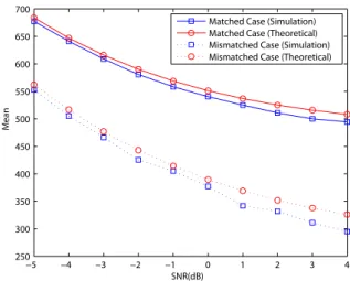
−5 −4 −3 −2 −1 0 1 2 3 4 250 300 350 400 450 500 550 600 650 700 SNR(dB) Mean
Matched Case (Simulation) Matched Case (Theoretical) Mismatched Case (Simulation) Mismatched Case (Theoretical)
Fig. 4. The means of𝐹𝑖,𝑚in a multipath Rayleigh fading channel with two equal-power paths when𝑁 = 512, 𝜖 = 0, and 𝜏 = 4.
is a Gaussian distribution with zero mean, one can derive the following terms by applying the mentioned property.
⎧ ⎨ ⎩ 𝐸{𝑅𝑒2{ ¯𝐻𝑙 0(𝑘)}} = 𝜎2 ℎ𝑙0 2 𝐸{𝑅𝑒2{ ¯𝐻 𝐿−1(𝑘)}} =𝜎 2 ℎ𝐿−1 2 𝐸{𝑅𝑒2{𝑊 (𝑘)}} = 𝜎2 𝑤 2 𝐸{𝑅𝑒2{𝑊 (𝑘 + 1)}} = 𝜎𝑤2 2 𝐸{𝑅𝑒2{𝑊 (𝑘 + 2)}} = 𝜎2 𝑤 2 . (36)
Therefore, after substituting (30) and (36) into (35) directly, (35) can be reduced to 𝜎2 𝑅𝑒{𝑆𝑖,𝑚(𝑘)}= ⎧ ⎨ ⎩ 9 2× (𝑁 sin(sin(𝜋𝜖)𝜋𝜖 𝑁)) 2× 𝜎2 ℎ𝑙0 +9 2× (𝑁 sin(sin(𝜋𝜖)𝜋𝜖 𝑁)) 2× 𝜎2 ℎ𝐿−1+32𝜎2𝑤, if 𝑖 = 𝑚 3 2× (𝑁 sin(sin(𝜋𝜖)𝜋𝜖 𝑁)) 2× 𝜎2 ℎ𝑙0 +3 2× (𝑁 sin(sin(𝜋𝜖)𝜋𝜖 𝑁)) 2× 𝜎2 ℎ𝐿−1+32𝜎2𝑤, if 𝑖 ∕= 𝑚. (37)
Similarly, the variance of𝐼𝑚{𝑆𝑖,𝑚(𝑘)}, 𝜎𝐼𝑚{𝑆2 𝑖,𝑚(𝑘)}, can be
obtained through the same derivation.
D. The distribution of𝐹𝑖,𝑚
With the definition of𝐹𝑖,𝑚in (27), by substituting (37) into
(32) and (33), the mean and variance of𝐹𝑖,𝑚 are
𝜇𝐹𝑖,𝑚= 𝑁−3∑ 𝑘=0 𝜇∥𝑆𝑖,𝑚(𝑘)∥ (38) and 𝜎2 𝐹𝑖,𝑚= 𝑁−3∑ 𝑘=0 𝜎2 ∥𝑆𝑖,𝑚(𝑘)∥ + 2 × 𝑁−3∑ 𝑘1,𝑘2=0;𝑘1<𝑘2 𝜌𝑖,𝑚(𝑘1, 𝑘2)𝜎∥𝑆𝑖,𝑚(𝑘1)∥𝜎∥𝑆𝑖,𝑚(𝑘2)∥,(39)
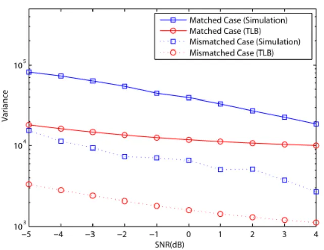
−5 −4 −3 −2 −1 0 1 2 3 4 103 104 105 SNR(dB) Variance
Matched Case (Simulation) Matched Case (TLB) Mismatched Case (Simulation) Mismatched Case (TLB)
Fig. 5. The variances of𝐹𝑖,𝑚in a multipath Rayleigh fading channel with two equal-power paths when𝑁 = 512, 𝜖 = 0, and 𝜏 = 4.
−5 −4 −3 −2 −1 0 1 2 3 250 300 350 400 450 500 550 600 650 SNR(dB)
Mean of Proposed Metric
Matched Case (Simulation) Matched Case (Theoretical) Mismatched Case (Simulation) Mismatched Case (Theoretical)
Fig. 6. The means of𝐹𝑖,𝑚 in a multipath Rayleigh fading channel with two equal-power paths when𝑁 = 512, 𝜖 = 0.4, and 𝜏 = 4.
respectively, where𝜌𝑖,𝑚(𝑘1, 𝑘2) is the correlation coefficient
between∥ 𝑆𝑖,𝑚(𝑘1) ∥ and ∥ 𝑆𝑖,𝑚(𝑘2) ∥. Since 𝜎∥𝑆𝑖,𝑚(𝑘)∥ is
the same for all subcarriers,𝜎2
𝐹𝑖,𝑚 can be further reduced to
𝜎2 𝐹𝑖,𝑚= 𝑁−3∑ 𝑘=0 𝜎2 ∥𝑆𝑖,𝑚(𝑘)∥ +2𝜎2 ∥𝑆𝑖,𝑚(𝑘)∥× 𝑁−3∑ 𝑘1,𝑘2=0;𝑘1<𝑘2 𝜌𝑖,𝑚(𝑘1, 𝑘2), (40)
For the simplification of the second component in (40),
we assume a common correlation coefficient ¯𝜌𝑖,𝑚 instead
of determining each distinct 𝜌𝑖,𝑚(𝑘1, 𝑘2). Since there are
correlatedness between the adjacent subcarriers, each distinct
𝜌𝑖,𝑚(𝑘1, 𝑘2) will be higher than the common correlation
co-efficient. That is, ∑𝑁−3𝑘
1,𝑘2=0;𝑘1<𝑘2𝜌𝑖,𝑚(𝑘1, 𝑘2) will be higher than(𝑁−2)(𝑁−3)¯𝜌𝑖,𝑚
2 . Hence, the following variance derivation
represents the lower bound of the proposed method and (40)
−5 −4 −3 −2 −1 0 1 2 3
103
104
105
SNR(dB)
Variance of Proposed Metric
Matched Case (Simulation) Matched Case (TLB) Mismatched Case (Simulation) Mismatched Case (TLB)
Fig. 7. The variances of𝐹𝑖,𝑚in a multipath Rayleigh fading channel with two equal-power paths when𝑁 = 512, 𝜖 = 0.4, and 𝜏 = 4.
can be rewritten as 𝜎2 𝐹𝑖,𝑚 ≥ 𝑁−3∑ 𝑘=0 𝜎2 ∥𝑆𝑖,𝑚(𝑘)∥+ (𝑁 − 2)(𝑁 − 3)𝜎∥𝑆2 𝑖,𝑚(𝑘)∥¯𝜌𝑖,𝑚. (41) By applying the method of Pearson product-moment cor-relation coefficient [18] and from simulation, the common
correlation coefficients, ¯𝜌𝑖,𝑚, can be approximated as
¯𝜌𝑖,𝑚≈
{
0.13, if 𝑖 = 𝑚
0.03, if 𝑖 ∕= 𝑚. (42)
Finally, by substituting (32) and (37) into (38), one can obtain
the following mean of𝐹𝑖,𝑚
𝜇𝐹𝑖,𝑚= ⎧ ⎨ ⎩ (𝑁 − 2) × ((36𝜎2ℎ0+36𝜎2ℎ𝐿−1)×(𝑁 sin( 𝜋𝜖sin(𝜋𝜖)𝑁 ))2+12𝜎2𝑤 𝜋 ) 1 2, if𝑖 = 𝑚 (𝑁 − 2) × ((12𝜎2ℎ0+12𝜎2ℎ𝐿−1)×(𝑁 sin( 𝜋𝜖sin(𝜋𝜖)𝑁 ))2+12𝜎2𝑤 𝜋 ) 1 2, if𝑖 ∕= 𝑚. (43) On the other hand, by substituting (33) and (37) into (41), the
lower bound of the variance of𝐹𝑖,𝑚 can be shown to be
𝜎2 𝐹𝑖,𝑚 ≥ ⎧ ⎨ ⎩ (𝑁2¯𝜌𝑖,𝑚− 5𝑁 ¯𝜌𝑖,𝑚+ 6¯𝜌𝑖,𝑚+ 𝑁 − 2) × (1 − 2 𝜋) ×{(9𝜎2 ℎ0+ 9𝜎ℎ2𝐿−1) × ( sin(𝜋𝜖) 𝑁 sin(𝜋𝜖 𝑁)) 2+ 3𝜎2 𝑤}, if 𝑖 = 𝑚 (𝑁2¯𝜌𝑖,𝑚− 5𝑁 ¯𝜌𝑖,𝑚+ 6¯𝜌𝑖,𝑚+ 𝑁 − 2) × (1 − 2 𝜋) ×{(3𝜎2 ℎ0+ 3𝜎ℎ2𝐿−1) × ( sin(𝜋𝜖) 𝑁 sin(𝜋𝜖 𝑁)) 2+ 3𝜎2 𝑤}, if 𝑖 ∕= 𝑚. (44) Although the above theoretical analysis focuses on the case with𝑅 = 3 and 𝑎𝑟= 1, it still can provide some ideas about
the performances under different𝑅s and 𝑎𝑟s intuitively. Since
(30) depends on𝑅, a larger 𝑅 will result in a larger difference
between the results of𝑖 = 𝑚 and 𝑖 ∕= 𝑚 in (30) than the case
with a smaller 𝑅. For examples, when 𝑅 = 4, the results of
𝑖 = 𝑚 and 𝑖 ∕= 𝑚 in (30) will become 16 × (𝑁 sin(sin(𝜋𝜖)𝜋𝜖
𝑁))
2
and 4 × (𝑁 sin(sin(𝜋𝜖)𝜋𝜖
𝑁))
TABLE I
COMPLEXITIES OF THEPROPOSEDMETHODS ANDCOMPLEXITYCOMPARISON
Techniques No. of Real-number No. of Real-number No. of Absolute-value Multiplication Operations Addition Operations Operations
Differential Autocorrelation Method (13) 4𝑀 × (𝑁 − 2) + 4𝑀 4𝑀 × (𝑁 − 2) + 2𝑀 𝑀
Differential Autocorrelation Method (14) 4𝑀 × (𝑁 − 2) + 8𝑀 4𝑀 × (𝑁 − 2) + 4𝑀 0 Differential Autocorrelation Method (45) 4𝑀 × (𝑁 − 2) + 4𝑀 4𝑀 × (𝑁 − 2) + 3𝑀 0
Proposed CERCD-I method 0 5𝑀 × (𝑁 − 3) + 4𝑀 𝑀 × (𝑁 − 3) + 𝑀
Proposed CERCD-II method 4𝑀 × (𝑁 − 3) + 4𝑀 7𝑀 × (𝑁 − 3) + 6𝑀 0
Proposed CERCD-III method 0 6𝑀 × (𝑁 − 3) + 5𝑀 0
difference between𝑖 = 𝑚 and 𝑖 ∕= 𝑚 is larger than the case
with 𝑅 = 3. Obviously, a larger difference will achieve a
better performance than a smaller one. Besides, same𝑎𝑟on all
𝑀𝑖,𝑚(𝑘)s is a reasonable choice so that the contributions from
all the𝑋𝑖,𝑚(𝑘) terms to ¯𝑋𝑖,𝑚,𝑙(𝑘) can be equally considered.
Fig. 4 shows the theoretically derived mean and the
simu-lated mean of𝐹𝑖,𝑚, while Fig. 5 shows the simulated variance
curves of𝐹𝑖,𝑚due to the matched and mismatched cases, and
the theoretical lower bound (TLB) of the variance. Moreover, Fig. 6 and Fig. 7 show similar results under the residual
frequency offset𝜖 = 0.4 in contrast to the residual frequency
offset𝜖 = 0 as in Fig. 4 and Fig. 5. In the figures, the matched
case means𝑖 = 𝑚, while the mismatched case means 𝑖 ∕= 𝑚.
As observed, regardless of the matched or mismatched cases, the curves of theoretically derived means are very close to the simulation means, while the simulated variances are bounded by the TLBs.
Moreover, by comparing Fig. 4 with Fig. 6, the difference between the means of the matched and the mismatched cases is smaller when there is a higher residual frequency offset in the system. Next, for evaluating the proposed methods, the comparisons of the complexity and the performance between the proposed techniques and the differential autocorrelation techniques will be discussed in the following two sections.
E. Probability of the Incorrect Cell ID Detection
For the probability of the incorrect cell ID detection, it is reasonable to treat the problem of finding the correct cell ID as a hypothesis testing problem. As such, the probability of the incorrect cell ID detection is
𝑃𝐼𝑛𝑐= 1 −
𝑀−1∏ 𝑚=0,𝑚∕=𝑖
𝑃 𝑟{𝐹𝑖,𝑚≤ 𝐹𝑖,𝑖}
Note that each∣∣𝑆𝑖,𝑚(𝑘)∣∣ in 𝐹𝑖,𝑚 is a random variable with
folded normal distribution. However, the adjacent∣∣𝑆𝑖,𝑚(𝑘)∣∣s
(i.e.,∣∣𝑆𝑖,𝑚(𝑘)∣∣, ∣∣𝑆𝑖,𝑚(𝑘+1)∣∣, ..., and ∣∣𝑆𝑖,𝑚(𝑘+𝑅−1)∣∣) are
not independent, because all of those terms partly contain the
same𝑀𝑖,𝑚(𝑘) terms. Thus, one cannot utilize the central limit
theorem (CLT) to model𝐹𝑖,𝑚 (which is a linear combination
of∣∣𝑆𝑖,𝑚(𝑘)∣∣) as a Gaussian random variable. As such, it is
not that easy and direct to obtain the probability density
func-tion (PDF) of𝐹𝑖,𝑚, that is, the exact theoretical probability
of the incorrect detection. Nevertheless, the discussion about the mean and variance still can exhibit the characteristics of the proposed methods. Especially, if one tries to practically
realize the proposed methods with fixed-point operations, those analyses can provide some guidelines about the word-length decision in the implementation.
V. COMPUTATIONALCOMPLEXITYANALYSIS
First of all, for a fair discussion, similar to the proposed CERCD-III method, the conventional differential autocorrela-tion technique in (13) can be also simplified as
ˆ𝑖 = arg max0≤𝑚≤𝑀−1∥∑𝑁−2𝑘=0 𝑀𝑖,𝑚(𝑘)𝑀𝑖,𝑚∗ (𝑘) ∥
= arg max0≤𝑚≤𝑀−1(∣𝑅𝑒{∑𝑁−2𝑘=0 𝑀𝑖,𝑚(𝑘)𝑀𝑖,𝑚∗ (𝑘)}
+ ∣𝐼𝑚{∑𝑁−2𝑘=0 𝑀𝑖,𝑚(𝑘)𝑀𝑖,𝑚∗ (𝑘)})
(45) Table I shows the complexity comparison of the conven-tional and proposed methods. Note that the complexity of each matching operation in (7) is negligible, because the preambles are assumed BPSK-modulated and each matching operation is equivalent to an exclusive-or (XOR) operation of sign bits. The conventional schemes need one complex multiplication
in computing 𝑀𝑖,𝑚(𝑘)𝑀𝑖,𝑚∗ (𝑘 + 1), while all the proposed
methods only require two complex additions in calculating
𝑆𝑖,𝑚(𝑘).
Moreover, the original form of the conventional methods
(i.e., (13)) requires 𝑀 absolute-value operations and each
∣(.)∣2 operation requires two real-number square operations
and a real-number addition operation, while (45) requires
a real-number addition operation to perform each ∥ (.) ∥
operation. As for the proposed methods, each ∣𝑆𝑖,𝑚(𝑘)∣ in
CERCD-I method costs four real-number addition operations and an absolute-value operation, while CERCD-II method requires two real-number multiplication operations and five
real-number addition operations for each ∣𝑆𝑖,𝑚(𝑘)∣2. Finally,
each ∥ 𝑆𝑖,𝑚(𝑘) ∥ in CERCD-III method is realized by five
real-number addition operations.
As shown in Table I, the number of multiplication oper-ations of the proposed CERCD-II method is less than the conventional methods of (14) and (45), while the number of additions of the proposed CERCD-II method is more than that of the conventional methods. However, by applying the approximation of (24) to the new metric, the proposed CERCD-III method does not require any multiplication op-eration. Hence, the proposed CERCD-III method has much lower complexity than all the other methods.
VI. SIMULATIONRESULTS
As mentioned in the introduction, since the current OFDM cell ID methods are all mainly based on the differential autocorrelation technique, the simulations results apply to all the discussed conventional non-coherent methods. For a rigorous assessment of the proposed and the conventional differential autocorrelation techniques, simulation results in different channel conditions are provided. Here, the system simulation parameters are defined as:
∙ Operating Frequency: 2.5 GHz
∙ Signal Bandwidth: 5 MHz
∙ FFT Length: 512
∙ Cyclic Prefix Length: 128
∙ Residual Timing Offset (𝜏): 4 samples
∙ Residual Frequency Offsets (𝜖): 0 or 0.4
∙ Normalized Doppler Frequency: 0.1
where the normalized Doppler frequency is equal to the maximum Doppler frequency normalized by the subcarrier spacing.
The simulation channel is based on Jake’s Rayleigh fading channel model [17]. The adopted power delay profiles with six paths follow the vehicular test environments of ITU-R model [15] as follows.
∙ Vehicular A channel (Power(dB)/Delay(𝑛𝑠)):
0dB/0𝑛𝑠, −1dB/310𝑛𝑠, −9dB/710𝑛𝑠,
−10dB/1090𝑛𝑠, −15dB/1730𝑛𝑠, −20dB/2510𝑛𝑠
∙ Vehicular B channel (Power(dB)/Delay(𝑛𝑠)):
−2.5dB/0𝑛𝑠, 0dB/300𝑛𝑠, −12.8dB/8900𝑛𝑠,
−10dB/12900𝑛𝑠, −25.2dB/17100𝑛𝑠, −16dB/20000𝑛𝑠,
According to power delay profile, the r.m.s. delay spreads of the vehicular A channel and the vehicular B channel
are 370.39𝑛𝑠 and 4001.4𝑛𝑠, respectively. Furthermore, the
coherent bandwidth of A channel and B channel are
approx-imately 539.97kHz and 49.98kHz, respectively. Since those
two bandwidths are all narrower than the signal bandwidth, both channels are frequency-selective fading channels. More-over, channel B is more frequency-selective than channel A, because its coherent bandwidth is narrower than that of A channel.
As shown in Fig. 8, the CERCD-I method with overlapping segments (corresponding to "Overlapping" in the legend of the figure) have better performances than the code group identification methods with non-overlapping segments in [21] (corresponding to "Non-overlapping" in the legend of the figure). In comparison with [21], when there is a code match, the proposed CERCD-I method actually performs filtering operation over the channel frequency responses, then takes absolute value of each output data sample of the filtering operation, and finally sums up all these absolute output data samples. In fact, the filtering operation is equivalent to a lowpass averaging operation over the channel responses. Here, by using a short window length (i.e., 3 in our algorithm demonstration), the proposed methods can better resist the adverse channel variation, because the consecutive subcarrier frequency responses within the short window length will be much more flatter than the much wider accumulation length in [21]. Since the proposed methods provide more average
sum terms (due to overlapped use of 𝑀𝑖,𝑚(𝑘) terms) with
1 2 3 4 5 6 7 8 9
10−2 10−1 100
SNR(dB)
Prob. of Incorrect Detection
R=3 (Overlapping) R=3 (Non−overlapping) R=6 (Overlapping) R=6 (Non−overlapping)
Fig. 8. The probability of the incorrect cell ID detection in a 6-path Rayleigh fading channel of the ITU-R vehicular A channel model (𝑓𝑛𝑑= 0.1).
−5 −4 −3 −2 −1 0 1 2 3 4 5 10−3 10−2 10−1 100 SNR (dB)
Probability of Incorrect Detection
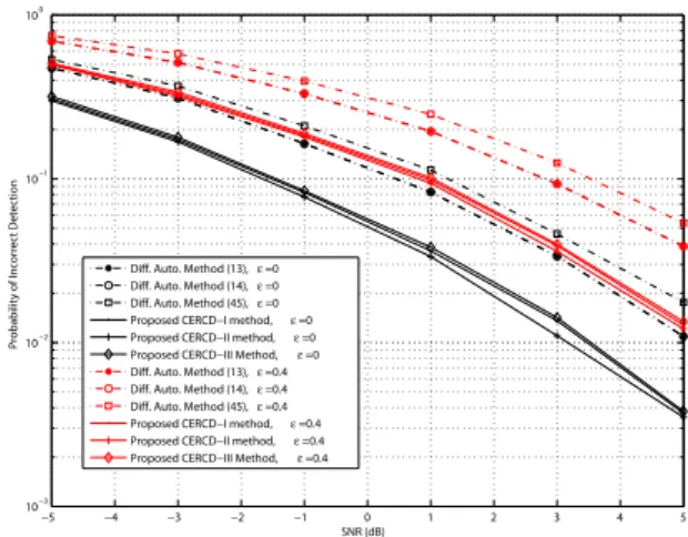
Diff. Auto. Method (13), ε =0 Diff. Auto. Method (14), ε =0 Diff. Auto. Method (45), ε =0 Proposed CERCD−I method, ε =0 Proposed CERCD−II method, ε =0 Proposed CERCD−III Method, ε =0 Diff. Auto. Method (13), ε =0.4 Diff. Auto. Method (14), ε =0.4 Diff. Auto. Method (45), ε =0.4 Proposed CERCD−I method, ε =0.4 Proposed CERCD−II method, ε =0.4 Proposed CERCD−III Method, ε =0.4
Fig. 9. The probability of the incorrect cell ID detection in a 6-path Rayleigh fading channel of the ITU-R vehicular A channel model..
small channel variations (due to short window length) than the method in [21] (with long window length and nonoverlapped
use of𝑀𝑖,𝑚(𝑘) terms), higher integration gain can be obtained
from the proposed methods than the method in [21], when the channel frequency responses vary noticeably over the subcarrier range, for examples, for non-flat channel responses or frequency selective channels. Hence, the proposed methods
with overlapping𝑀𝑖,𝑚(𝑘)s are more robust against non-flat
channel conditions and burst error than the method with
non-overlapping𝑀𝑖,𝑚(𝑘)s in [21].
Fig. 9 and Fig. 10 show the simulation results under channel A and channel B with different residual frequency
offsets (i.e., 𝜖 = 0 and 𝜖 = 0.4), respectively. Note that
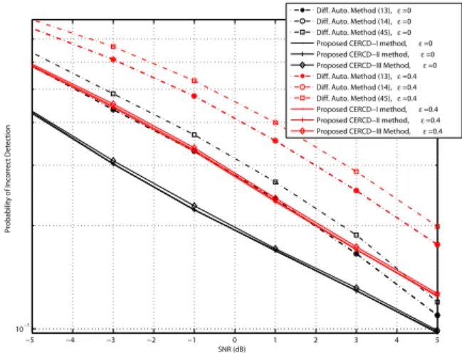
the "Diff. Auto. Method", appearing in the legends of those figures, means the conventional differential autocorrelation method. In the figures, the probabilities of the incorrect cell ID detection are compared. As shown, regardless of SNR and channel conditions, all the proposed methods exhibit better performances than the conventional differential autocorrelation methods whatever the residual frequency offset is.
−5 −4 −3 −2 −1 0 1 2 3 4 5 10−1
SNR (dB)
Probability of Incorrect Detection
Diff. Auto. Method (13), ε =0 Diff. Auto. Method (14), ε =0 Diff. Auto. Method (45), ε =0 Proposed CERCD−I method, ε =0 Proposed CERCD−II method, ε =0 Proposed CERCD−III Method, ε =0 Diff. Auto. Method (13), ε =0.4 Diff. Auto. Method (14), ε =0.4 Diff. Auto. Method (45), ε =0.4 Proposed CERCD−I method, ε =0.4 Proposed CERCD−II method, ε =0.4 Proposed CERCD−III Method, ε =0.4
Fig. 10. The probability of the incorrect cell ID detection in a 6-path Rayleigh fading channel of the ITU-R vehicular B channel model.
Beside, in figures, the performance differences among the proposed methods are almost negligible. Let us first consider CERCD-I and CERCD-II methods. Although the performance of CERCD-II is conceptually better than CERCD-I as dis-cussed in Section III, their difference is not much in the
simulation, because a matched ∣𝑆𝑖,𝑚(𝑘)∣ with a large value
in CERCD-I method automatically guarantees a large-value
∣𝑆𝑖,𝑚(𝑘)∣2 in CERCD-II method, and vice versa. Therefore,
both methods generate similar results in the maximum-value
search process (i.e.,𝑎𝑟𝑔𝑚𝑎𝑥). Next, let us consider
CERCD-I and CERCD-CERCD-ICERCD-ICERCD-I methods. Since ∣∣𝑆𝑖,𝑚(𝑘)∣∣ of
CERCD-III method is a simplified version of the absolute operation
∣𝑆𝑖,𝑚(𝑘)∣ of CERCD-I method and ∣∣𝑆𝑖,𝑚(𝑘)∣∣ is always
larger than or equal to ∣𝑆𝑖,𝑚(𝑘)∣, a large matched ∣𝑆𝑖,𝑚(𝑘)∣
value in CERCD-I method also automatically guarantees a
large matched∣∣𝑆𝑖,𝑚(𝑘)∣∣ value in CERCD-III method, like in
the comparison discussion between I and CERCD-II methods. Hence, both methods also have very close
per-formance. However, a small-value unmatched ∣𝑆𝑖,𝑚(𝑘)∣ in
CERCD-I method does not necessarily imply a small-value
∣∣𝑆𝑖,𝑚(𝑘)∣∣ in CERCD-III method. In this case, it will cause
performance degradation of CERCD-III method. As such, performance of CERCD-III is inferior but close to that of CERCD-I method.
For the conventional methods, the reason why the
per-formance of the absolute operation ∣(.)∣ in (13) is close
to that of the square absolute operation ∣(.)∣2 in (14) is
the same as explained in the comparison of CERCD-I and CERCD-II methods. Since conventional methods take the absolute value operation after the entire differential
auto-correlation operation, i.e.,∣∑𝑁−2𝑘=0 𝑀𝑖,𝑚(𝑘)𝑀𝑖,𝑚∗ (𝑘 + 1)∣, the
conventional method of (45) have larger performance differ-ences from (13) and (14) than the differdiffer-ences of CERCD-III from CERCD-I and CERCD-II methods. As previously discussed, note that the conventional methods accumulate the
𝑀𝑖,𝑚(𝑘)𝑀𝑖,𝑚∗ (𝑘 + 1) terms in the entire subcarrier range.
Hence, conventional methods are subject to channel vari-ations. On the other hand, the proposed methods are less influenced by channel variation effects, because the basic
smoothing term of∣𝑀𝑖,𝑚(𝑘) + 𝑀𝑖,𝑚(𝑘 + 1) + 𝑀𝑖,𝑚(𝑘 + 2)∣
is operated in a limited local range. Due to the much longer accumulation range than that of CERCD-III method,
the approximation error of∣∣∑𝑁−2𝑘=0 𝑀𝑖,𝑚(𝑘)𝑀𝑖,𝑚∗ (𝑘 + 1)∣∣ to
∣∑𝑁−2𝑘=0 𝑀𝑖,𝑚(𝑘)𝑀𝑖,𝑚∗ (𝑘 + 1)∣ will be much larger than the
error between CERCD-I and CERCD-III methods. Hence, one can see a large difference between (45) and (13) or (14) than the difference between III and I or CERCD-II methods.
Next, we will discuss the performances of the conventional and proposed methods. For conventional methods, the
ba-sic accumulation term 𝑀𝑖,𝑚(𝑘)𝑀𝑖,𝑚∗ (𝑘 + 1) in differential
autocorrelation supposedly can cancel the channel phases
of the 𝑘-th and (𝑘 + 1)-th preamble subcarriers, given
that 𝐻(𝑘) ≈ 𝐻(𝑘 + 1). As a result, 𝑀𝑖,𝑚(𝑘)𝑀𝑖,𝑚∗ (𝑘 +
1) reduces to either ∣𝐻(𝑘)∣2 or −∣𝐻(𝑘)∣2 regardless of
whether there is a code match or not. When there is a
code match, then all the 𝑀𝑖,𝑚(𝑘)𝑀𝑖,𝑚∗ (𝑘 + 1) terms will
produce the squared channel response magnitudes with the
same sign. Then by accumulating all the 𝑀𝑖,𝑚(𝑘)𝑀𝑖,𝑚∗ (𝑘 +
1) terms, i.e., ∑𝑁−2𝑘=0 𝑀𝑖,𝑚(𝑘)𝑀𝑖,𝑚∗ (𝑘 + 1), one can
ob-tain a significantly large absolute autocorrelation value
(i.e., ∣∑𝑁−2𝑘=0 𝑀𝑖,𝑚(𝑘)𝑀𝑖,𝑚∗ (𝑘 + 1)∣ is approximately equal
to ∑𝑁−2𝑘=0 ∣𝐻(𝑘)∣2). On the other hand, when there is no
code match, the signs of 𝑀𝑖,𝑚(𝑘)𝑀𝑖,𝑚∗ (𝑘 + 1) will vary
with 𝑘 randomly so that one will obtain a much smaller
∣∑𝑁−2𝑘=0 𝑀𝑖,𝑚(𝑘)𝑀𝑖,𝑚∗ (𝑘 + 1)∣ value than the matched case.
Since conventional methods assume equal channel responses
at two consecutive preamble subcarriers, i.e.,𝐻(𝑘) ≈ 𝐻(𝑘 +
1), their performances will be poor if the channel variation is high and the phase difference between these two subcar-riers’ channel frequency responses will not be small so that
one will not expect either ∣𝐻(𝑘)∣2 or −∣𝐻(𝑘)∣2 value from
𝑀𝑖,𝑚(𝑘)𝑀𝑖,𝑚∗ (𝑘 + 1). Under this condition the accumulation
value of∣∑𝑁−2𝑘=0 𝑀𝑖,𝑚(𝑘)𝑀𝑖,𝑚∗ (𝑘 + 1)∣ will be much less than
the cases under small channel variations.
On the other hand, the proposed methods actually
per-forms channel response smoothing operation, i.e., 𝑆𝑖,𝑚(𝑘) =
𝑀𝑖,𝑚(𝑘) + 𝑀𝑖,𝑚(𝑘 + 1) + ... + 𝑀𝑖,𝑚(𝑘 + 𝑅) = 𝐻(𝑘) +
𝐻(𝑘 + 1) + ... + 𝐻(𝑘 + 𝑅), when there is a code match.
Thus, the proposed methods can obtain a large matched value
of∑𝑁−𝑅𝑘=0 ∣𝑆𝑖,𝑚(𝑘)∣. However, when there is no code match,
value of 𝑀𝑖,𝑚(𝑘) + 𝑀𝑖,𝑚(𝑘 + 1) + ... + 𝑀𝑖,𝑚(𝑘 + 𝑅) can
randomly be any one of the2𝑅possible results (depending on
𝑘): ±𝐻(𝑘)±𝐻(𝑘 +1)±...±𝐻(𝑘 +𝑅). As such, it leads to a
smaller mismatched value of∑𝑁−𝑅𝑘=0 ∣𝑆𝑖,𝑚(𝑘)∣. Consequently,
one can see that the proposed methods do not utilize the channel phase differential operations used by conventional differential autocorrelation methods, in the cell ID detection. Without relying on differential phase technique and assuming equal channel phases of two consecutive subcarriers, the proposed methods are less influenced by the channel response variations. Hence, the proposed methods have better perfor-mances than the conventional autocorrelation-based methods as illustrated in Fig. 9 and Fig. 10.
In addition, for reducing the computational complexities and further generalizing the optimization metrics, one can
−5 −4 −3 −2 −1 0 1 2 3 4 5 1 3 5 10−2 10−1 Decimation Factor SNR (dB)
Probability of Incorrect Detection
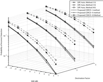
Diff. Auto. Method (13) Diff. Auto. Method (14) Diff. Auto. Method (45) Proposed CERCD−I method Proposed CERCD−II method Proposed CERCD−III Method
Fig. 11. The probability of the incorrect cell ID detection in a 6-path Rayleigh fading channel of the ITU-R vehicular A channel model, under different decimation factors, when𝜖 = 0 and 𝜏 = 4.
methods as follows.
∙ Generalized Differential Autocorrelation Method of (13):
ˆ𝑖 = arg max0≤𝑚≤𝑀−1 ∣∑⌊ 𝑁−2 𝑑 ⌋ 𝑘=0 𝑀𝑖,𝑚(𝑘 × 𝑑) ×𝑀∗ 𝑖,𝑚(𝑘 × 𝑑 + 1)∣
∙ Generalized Differential Autocorrelation Method of (14):
ˆ𝑖 = arg max0≤𝑚≤𝑀−1 ∣∑⌊ 𝑁−2 𝑑 ⌋ 𝑘=0 𝑀𝑖,𝑚(𝑘 × 𝑑) 𝑀∗ 𝑖,𝑚(𝑘 × 𝑑 + 1)∣2
∙ Generalized Differential Autocorrelation Method of (45):
ˆ𝑖 = arg max0≤𝑚≤𝑀−1 ∥∑⌊ 𝑁−2 𝑑 ⌋ 𝑘=0 𝑀𝑖,𝑚(𝑘 × 𝑑) 𝑀∗ 𝑖,𝑚(𝑘 × 𝑑 + 1) ∥
∙ Generalized CERCD-I Method:
ˆ𝑖𝐼 = arg0≤𝑚≤𝑀−1max ⌊𝑁−3 𝑑 ⌋ ∑ 𝑘=0 ∣𝑆𝑖,𝑚(𝑘 × 𝑑)∣
∙ Generalized CERCD-II Method:
ˆ𝑖𝐼𝐼 = arg0≤𝑚≤𝑀−1max ⌊𝑁−3 𝑑 ⌋ ∑ 𝑘=0 ∣𝑆𝑖,𝑚(𝑘 × 𝑑)∣2
∙ Generalized CERCD-III Method:
ˆ𝑖𝐼𝐼𝐼 = arg0≤𝑚≤𝑀−1max ⌊𝑁−3 𝑑 ⌋ ∑ 𝑘=0 ∥ 𝑆𝑖,𝑚(𝑘 × 𝑑) ∥
Note that ⌊ ⌋ is the floor function, the decimation factor 𝑑
is a positive integer. As shown in the generalized methods,
only one subcarrier out of every𝑑 subcarriers is included in
the accumulation of optimization functions. Consequently, one can do the tradeoff between complexities and performances of those methods in practical applications.
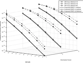
Fig. 11 and Fig. 12 show the performances of the
con-ventional and proposed methods when decimation factor𝑑 =
1, 3, 5, residual frequency offset 𝜖 = 0, 𝑅 = 3, and all the
weighting coefficients 𝑎𝑟 = 1. Note that the performances
of the conventional and proposed methods when 𝑑 = 1 in
−5 −4 −3 −2 −1 0 1 2 3 4 5 1 3 5 10−1 Decimation Factor SNR (dB)
Probability of Incorrect Detection
Diff. Auto. Method (13) Diff. Auto. Method (14) Diff. Auto. Method (45) Proposed CERCD−I method Proposed CERCD−II method Proposed CERCD−III Method
Fig. 12. The probability of the incorrect cell ID detection in a 6-path Rayleigh fading channel of the ITU-R vehicular B channel model, under different decimation factors, when𝜖 = 0 and 𝜏 = 4.
−5 −4 −3 −2 −1 0 1 2 3 4 5 1 3 5 10−1 Decimation Factor SNR (dB)
Probability of Incorrect Detection
Diff. Auto. Method (13) Diff. Auto. Method (14) Diff. Auto. Method (45) Proposed CERCD−I method Proposed CERCD−II method Proposed CERCD−III Method
Fig. 13. The probability of the incorrect cell ID detection in a 6-path Rayleigh fading channel of the ITU-R vehicular A channel model, under different decimation factors, when𝜖 = 0.4 and 𝜏 = 4.
Fig. 11 and Fig. 12 are the same as in Fig. 9 and Fig. 10, respectively. In addition, regardless of decimation factors, Fig. 11 and Fig. 12 show that all the proposed methods have better performances than the conventional methods. Fig. 13 and Fig. 14 show the performances of those methods under vehicular A channel and vehicular B channel, respectively,
when the residual frequency offset 𝜖 = 0.4. In the presence
of the residual frequency offset, similar observation to Fig. 11 and Fig. 12 are obtained. That is, all the proposed methods work well and have better performance than the conventional methods.
VII. CONCLUSION
Based on the proposed new metric and its two simplifi-cations, three new non-coherent cell ID detection techniques and statistical analysis for cellular OFDM systems have been proposed in this work. All the proposed methods have better performances than the conventional methods. Especially, the complexity analysis and simulation results show that the proposed CERCD-III method has much lower complexity