運用考慮交互效果的真實固定效果模型探討各國總體生產效率

科技部補助專題研究計畫成果報告

期末報告

運用考慮交互效果的真實固定效果模型探討各國總體生產

效率

計 畫 類 別 ： 個別型計畫 計 畫 編 號 ： NSC 102-2410-H-004-009- 執 行 期 間 ： 102 年 08 月 01 日至 103 年 07 月 31 日 執 行 單 位 ： 國立政治大學金融系 計 畫 主 持 人 ： 黃台心 計畫參與人員： 學士級-專任助理人員：邱郁芳 處 理 方 式 ： 1.公開資訊：本計畫涉及專利或其他智慧財產權，2 年後可公開查詢 2.「本研究」是否已有嚴重損及公共利益之發現：否 3.「本報告」是否建議提供政府單位施政參考：否

中 華 民 國 103 年 10 月 15 日

中 文 摘 要 ： 本研究在 Greene (2005a, 2005b) and Wang and Ho (2010) 真實固定或隨機效果模型架構下，利用 Bai (2009) 所稱的 交互效果 (interactive effects) 將無法觀察到的共同衝擊 因子 (unobserved common shocks) 納入考量。分別探討我 國銀行業的技術效率以及各國總體生產效率。將這種無法觀 察到的共同衝擊因子納入迴歸模型，表示各國生產活動具有 橫斷面相依性與來自共同因子的異質衝擊。迴歸模型若忽略 這種交互效果，易造成係數與效率估計值的偏誤。

根據 Hsu et al. (2012) 發展的方法，利用 Pesaran (2006) 的方法先對迴歸模型進行轉換，設法消除交互效果， 再針對轉換後模型以最大概似法進行估計，就可得到具備一 致性的係數與效率估計值。研究對象為各國總體隨機生產邊 界函數，並進一步將樣本國家分成低與高所得兩群組，採用 Huang et al. (2014) 發展的新共同生產邊界模型進行生產 效率與生產力之比較。 研究結果發現這兩群組國家採用不同的生產技術進行生 產，確認應採用共同邊界模型估計和比較兩群組的生產效 率。此外，高所得國家的技術進步速度較低所得國家快且生 產技術較為接近固定規模報酬；然而低所得國家的總技術效 率優於高所得國家，主要原因為低所得國家的群組技術效率 高於高所得國家，兩群國家的技術缺口比率幾無差異。 中文關鍵詞： 真實固定效果模型； 交互效果； 共同衝擊因子；技術效 率；共同生產邊界模型；

英 文 摘 要 ： This paper applies the true fixed effects model of Greene (2005a, 2005b) and Wang and Ho (2010),

together with interactive effects of Bai (2009), to examine the production efficiency of countries. To compare efficiency scores of the sample countries, we suggest the use of the meta-production frontier, developed by Huang et al. (2014). The inclusion of the interactive effects allows us to explain why different countries (firms) might be influenced by various degrees of impacts coming from

observed/unobserved common economic/technology shocks. These effects are modeled as the product of firm-specific parameters (loadings) and common shocks (factors). The exclusion of these effects from models

may lead to bias parameter estimates and efficiency measures.

Following Hsu et al. (2012), we first employ the transformation procedure, proposed by Pesaran (2006), to purge the interactive effects, and then estimate the transformed model by the maximum likelihood. This leads to consistent parameter estimates and

efficiency scores. Panel data of aggregate output produced by labor and physical capital for countries are used to investigate issues related to production efficiency. The sample countries are further divided into two groups, i.e., low and high income countries. The low and high income countries are found to utilize different production technologies and to take the increasing returns to scale technology, but the latter countries are closer to the constant returns to scale. The speed of technical advance for high income countries is faster than that of low income countries. However, the overall technical efficiency score of low income countries is greater than that of high income countries, due mainly to technical

efficiency rather than TGR, while the difference between the two groups is not large.

英文關鍵詞： true fixed effects model； interactive effects； common shocks； technical efficiency； meta-production frontier；

1

行政院國家科學委員會補助專題

研究計畫

□期中進度報

告



期末報告

運用考慮交互效果的真實固定效果模型探討各

國總體生產效率

計畫類別：個別型計畫 □整合型計畫

計畫編號：NSC 102－2410－H－004－009－

執行期間： 102 年 8 月 1 日至 103 年 7 月 31 日

執行機構及系所：國立政治大學金融學系

計畫主持人： 黃台心

共同主持人：

計畫參與人員： 邱郁芳

本計畫除繳交成果報告外，另含下列出國報告，共 _0_ 份：

□移地研究心得報告

□出席國際學術會議心得報告

□國際合作研究計畫國外研究報告

處理方式：除列管計畫及下列情形者外，得立即公開查詢

□涉及專利或其他智慧財產權，□一年二年後可

公開查詢

中 華 民 國 103 年 10 月 15 日

2

中文摘要

本研究在 Greene (2005a, 2005b) and Wang and Ho (2010) 真實固定或隨機效 果模型架構下，利用 Bai (2009) 所稱的交互效果 (interactive effects) 將無法觀察 到的共同衝擊因子 (unobserved common shocks) 納入考量。分別探討我國銀行業 的技術效率以及各國總體生產效率。將這種無法觀察到的共同衝擊因子納入迴歸 模型，表示各國生產活動具有橫斷面相依性與來自共同因子的異質衝擊。迴歸模 型若忽略這種交互效果，易造成係數與效率估計值的偏誤。

根據 Hsu et al. (2012) 發展的方法，利用Pesaran (2006) 的方法先對迴歸模

型進行轉換，設法消除交互效果，再針對轉換後模型以最大概似法進行估計，就 可得到具備一致性的係數與效率估計值。研究對象為各國總體隨機生產邊界函數， 並進一步將樣本國家分成低與高所得兩群組，採用 Huang et al. (2014) 發展的新 共同生產邊界模型進行生產效率與生產力之比較。 研究結果發現這兩群組國家採用不同的生產技術進行生產，確認應採用共 同邊界模型估計和比較兩群組的生產效率。此外，高所得國家的技術進步速度較 低所得國家快且生產技術較為接近固定規模報酬；然而低所得國家的總技術效率 優於高所得國家，主要原因為低所得國家的群組技術效率高於高所得國家，兩群 國家的技術缺口比率幾無差異。 關鍵詞：真實固定效果模型； 交互效果； 共同衝擊因子；技術效率；共同生產 邊界模型；

3

Abstract

This paper applies the true fixed effects model of Greene (2005a, 2005b) and Wang and Ho (2010), together with interactive effects of Bai (2009), to examine the production efficiency of countries. To compare efficiency scores of the sample countries, we suggest the use of the meta-production frontier, developed by Huang et al. (2014). The inclusion of the interactive effects allows us to explain why different countries (firms) might be influenced by various degrees of impacts coming from observed/unobserved common economic/technology shocks. These effects are modeled as the product of firm-specific parameters (loadings) and common shocks (factors). The exclusion of these effects from models may lead to bias parameter estimates and efficiency measures.

Following Hsu et al. (2012), we first employ the transformation procedure, proposed by Pesaran (2006), to purge the interactive effects, and then estimate the transformed model by the maximum likelihood. This leads to consistent parameter estimates and efficiency scores. Panel data of aggregate output produced by labor and physical capital for countries are used to investigate issues related to production efficiency. The sample countries are further divided into two groups, i.e., low and high income countries.

The low and high income countries are found to utilize different production technologies and to take the increasing returns to scale technology, but the latter countries are closer to the constant returns to scale. The speed of technical advance for high income countries is faster than that of low income countries. However, the overall technical efficiency score of low income countries is greater than that of high income countries, due mainly to technical efficiency rather than TGR, while the difference between the two groups is not large.

Keywords: true fixed effects model; interactive effects; common shocks; technical efficiency; meta-production frontier;

4

目錄

I. Introduction………5

II. The Econometric Model………7

2.1 The Group Production Frontiers……….7

2.2 The Stochastic Meta-Frontier Production Function………10

III. Data………..13

IV. Empirical Results……….13

4.1 Group Frontiers……….13

4.1 The Meta-Production Frontier………..15

V. Conclusion………..18

5

Applying the True Fixed Effects Model with Interactive Effects to

Compare Production Efficiencies for Countries of Different Groups

I.

Introduction

The stochastic frontier (SF) approach, first developed by Aigner et al (1977) and Meeusen and van den Broeck (1977), has been extensively used to investigate

technical efficiency (TE) of firms and countries, using cross-sectional data. Schmidt and Sickles (1984) extend this approach to panel data context with fixed and random effects. Under the framework of fixed and random effects models, the individual heterogeneity is usually assumed to be time invariant and also represents technical inefficiency of the firm. Later, the time invariant technical inefficiency is relaxed by, e.g., Cornwell et al. (1990), Kumbhakar (1990), and Lee and Schmidt (1993), to mention a few. This mixture of heterogeneity with technical inefficiency obscures the true managerial ability for firms, since the resulting efficiency score may pick up heterogeneity. To solve this difficulty Greene (2005) proposes a true fixed-effect stochastic frontier model, in which the SF model with panel data includes both heterogeneity and inefficiency term. However, his model may suffer from the problem of incidental parameters. Wang and Ho (2010) suggest a class of panel stochastic frontier models that remove the individual effects by either taking the first difference or using the within estimation, which concurrently purge the heterogeneity and the incidental parameters problem.

The above works ignore the presence of cross-sectionally correlated error terms and consequently fail to explain why different firms (countries) are likely to be influenced by various degrees of effects incurred by unobserved common effects that cause cross section dependence. The common effects or interactive effects (Bai, 2009) is specified as a product of firm-specific parameters (loadings) and common shocks (factors). Since the common effects are allowed to be correlated with explanatory variables, the exclusion of them from a panel regression model may result in inconsistent parameter estimators. This arises from the fact that the error term contains the unobserved, excluded common shocks and hence is correlated with the regressors.

Several researchers devote to deal with this problem by either estimating or controlling for the interactive effects in linear regression models, e.g., Ahn et al. (2006), Pesaran (2006), and Bai (2009). The method, developed by Pesaran (2006), relies on the assumption of stationary panel regressions with a multifactor error structure; Pesaran (2011) generalizes to the case that allows the unobservable

6

common factors to follow unit root processes. It is well-known that many

macroeconomic time series, such as the GDP, monetary aggregates, the price level (CPI and GDP deflator), employment level, capital stock, etc., are characterized as non-stationary. The important finding by Pesaran (2011) is that the results of Pesaran (2006) continue to hold in the non-stationary case, which legitimates researchers applying his model to estimate, e.g., a country-level production function that involves the use of macro-economic time series.

Ahn et al. (2007) combine all unobservable common factors with the inefficiency

term in order to consistently estimate slope coefficients in a SF model. This appears to be questionable treating the interactive effects as a part of inefficiency, because the common factors are uncontrollable by the firm and therefore should not be associated with managerial abilities of the firm. In addition, one may mistakenly conclude that some regional and small banks exposure of less financial shocks outperform

international and large banks that suffer from more impacts, if interactive effects are considered as a portion of inefficiency. Following the vein of Pesaran (2006), Hsu et al. (2013) recently develop a technique that allows one to consistently estimate the SF model with common factors for large N (number of firms) and fixed T (number of time periods) panel. Their approach requires first transforming the regression model to filter out interactive effects, as proposed by Pesaran (2006, 2011), followed by estimating the transformed model by the maximum likelihood (ML) to obtain

consistent coefficient estimates, as well as efficiency scores. Monte Carlo simulations confirm that their approach is able to produce satisfactory finite sample properties.

To compare TEs of firms from different groups, some previous works simply estimate a meta-frontier by pooling all samples of various groups.1 This appears to be invalid, as the so-derived meta-frontier would not necessarily envelop the

group-specific frontiers. It would also lack justification if one first estimates the individual group frontiers and then compares the TEs among groups, since these TE scores are assessed relative to different production frontiers, instead of the

metafrontier. Battese et al. (2004) propose a metafrontier production function model that deals with the above difficulties. Their mixed approach consists of two steps to get the metafrontier. However, their second step estimation relies on the use of programming techniques that has no statistical properties of the derived metafrontier estimators. Moreover, programming techniques are unable to account for different production environments facing firms and isolate random shocks uncontrolled by firms. To correct the foregoing difficulties, Huang et al. (2014) newly develop a novel two-step SF approach whose second-step estimation of the metafrontier is still based on the SF framework. This stochastic metafrontier can be estimated by the ML such

7

that the conventional statistical inferences can be implemented without counting on simulations or bootstrapping.2

This paper introduces the procedure of Huang et al. (2014) to estimate

macro-production frontiers and compare TEs for countries of different groups. The salient feature of this paper is attributed to its inclusion of the interactive effects that account for heterogeneous impacts on individual countries of unobserved common shocks. Importantly, these common factors, along with unobserved heterogeneity, are purged at the outset so that the inefficiency term will not pick up the common effects and the incidental parameters problem is solved simultaneously. Viewed from this angle, the stochastic meta-frontier with common factors is theoretically advantageous over the deterministic meta-frontier of Battese et al. (2004) and O’Donnell et al. (2008).

The rest of the paper is organized as follows. Section 2 develops the econometric model. Section 3 describes the data and sample statistics. Section 4 analyzes empirical results, while the last section concludes the paper.

II.

The Econometric Model

2.1 The Group Production Frontiers

Following Hsu et al. (2013), the true fixed effect SF model with unobserved common effects for group j (=1,…, J) is specified as:

j j j j j j j i t i i t i t i t i t

y   X    f v u， i = 1,…, Nj; t = 1,…, T (1)

where y denotes the (log)output of the ith country at time t, _itj _ij is the individual heterogeneity, j

it

X is a k1 vector of (log)inputs, j is the corresponding coefficients, f_t contains r unobserved common factors, _ij is the corresponding

factor loadings,



2



~ 0,

j j

it v

v N  is the error term, and u is the time-varying _itj

inefficiency term. Here, X is allowed to be correlated with _itj _ij and the common factors, as suggested by Pesaran (2006, 2011) and Hsu et al. (2013).3 As a result, this specification accounts for both cross-sectional dependence and the correlation

2 _{Note that the first-step estimation procedure of Huang et al. (2014) is the same as Battese et al. (2004)}

and O’Donnell et al. (2008), in which the individual group frontiers are estimated.

3 _{Although Ahn et al. (2006, 2007) relate} j it

8

between common effects and regressors. The inefficiency term is assumed to include the scaling factor of Wang and Schmidt (2002) and Wang and Ho (2010), i.e., j



j j



*j

it it i

u h  z u (2)

where z is a vector of environmental variables affecting inefficiency, _itj j

is the

corresponding unknown coefficients, and u_ij* ~N



 j, _uj2



has a truncated normal distribution with a constant mean, j, and a constant variance, _uj2.4

The emergence of the interactive effects of _ijf_t captures the heterogeneous impacts of unobserved common shocks to countries. For example, the Asian financial crisis, occurred in the mid-1997, affects mainly those East Asian economies and other countries suffer from this crisis in a lesser extent. This model is capable of

distinguishing heterogeneous impacts on East Asian economies from the remaining economies through the term of _ijf_t. The subprime crisis of the U.S. in 2008 hits seriously the financial industry of the U.S and plagues many Western European countries later. Although this crisis also influences the global economy, other countries than the U.S and Western European countries undergo less and indirect unfavorable influences. The use of our maintained model can isolate such adverse effects from the inefficiency term and gives us better TE estimates.

Define the idempotent matrix of M_wj I_T H_wj



H H_wj _wj



1H_wj, where I_T is a

T T identity matrix, H_wj 



D Z h, _wj, _wj_**j



, D is a T1 vector of ones,



,



j j j w w w

Z  y X is the cross-sectional average of



y_ij,X_ij



using the weight w_ij for each time period, h is the cross-sectional average of _wj j

it

h using the same weight for

each time period, _**j j j



j / j

 

/ j / j



u u u

         is the mean value of u , _i* j

and 

 

 and  

 

are the probability density and cumulative distribution

9

functions, respectively.5 Note that matrix M has no full-rank. Its rank depends on _wj

the dimension of H and is equal to _wj Ts, where dim

 

j w s H .

Let _ij v_ij u_ij be a T1 vector. Multiplying equation (1) byM , we obtain _wj

j j j j j j j w i w i w i M y M X  M  (3) where j j ~



0, j



w i M v N  ,  j _vj2M_wj, and j j j



j j



*j w i w i i M u M h  z u . It is

noticeable that M is not invertible due its lack of full rank. Following Khatri (1968) _wj

and Harville (1997), one can at most obtain the generalized inverse of j, denoted by j. Hsu et al. (2012) derive the marginal log-likelihood function for firm i of the jth group:

 

2 *2 2 2 2 * * * * 1 1 1 ln ( ) ln 2 ln 2 2 2 ln ln j j j j j j j j j i v i w w i j j u j j j j u j j u L T s    M M                     _  _   _  _           _ _{ } _ _{ }         (4) where 2 * 2 / 1 / j j j j j j j j u i w w i j j j j j j i w w i u M M h h M M h               , (5) and _*2 1 ₂ 1 / j j j j j j j i w w i u h M M h        . (6)

where h is a _ij T1 vector. Summing lnL over all firms, one yields the _ij

log-likelihood function for the entire sample. Under certain conditions, Hsu et al. (2012) prove that the maximum likelihood estimators are consistent for fixed T and large N . Following the line of Jondrow et al. (1982) and Wang and Ho (2010), Hsu j

et al. (2012) suggest using the conditional expectation of u on the vector of _itj M_{w i}jj

as the measure of inefficiency index:

5 _{Assumption 5 of Pesaran (2006) states the conditions for the weight} j i w , i.e., (i) w_ij O



1 /Nj



, (ii) 1 1 N _j i i w 



, and (iii) 1 N _j i i w K



, where K .

10



 



* * * * * * | j j j j j j j j j it w i it j j E u M h z                                      (7)

The technical efficiency score is equal to TE_itj exp_E u



_itj|M_{w i}jj



_.6

2.2 The Stochastic Meta-Frontier Production Function

We construct the metafrontier ftM

 

Xjit that, by definition, envelops or lies

above all individual groups’ production frontiers ftj

 

Xitj , which can be formulated

as:

 

 

UMjit, , , j j M j t it t it f X  f X e j i t (8) where M 0 jit

U  denotes the gap between the metafrontier and the jth group’s frontier.7 Hence, M

 

. j

 

.

t t

f  f and the ratio of the jth group’s production frontier to the metafrontier is defined as the technology gap ratio (TGR),

 

 

Mjit 1 j j t it _U j it _{M j} t it f X TGR e f X     . (9)

The existence of the technology gap is attributed to the choice of a particular technology that depends on the economic and non-economic environments. The technology gap element M

jit

U in (9) varies across groups, firms, and time periods.

The value of the TGR reflects the accessibility and extent of acceptance of the available potential production technology. Readers are suggested to refer to Huang et al. (2014) for detailed treatment on the relationship between group frontiers and the metafrontier. In sum, the overall TE of the ith firm at time t in the jth group, MTE , _itj

6 _{Battese and Coelli (1988) propose another formula to compute TE directly, i.e.,}

 

exp | j j j j it it w i TE E u M  . 7 _{Note that} j

 

t j it

f X is equal to the exponent of the sum of the first three terms on the right-hand of (1).

11

relative to the metafrontier production frontier (adjusted by noise v ) can be _itj

expressed as:

 

j it j j it j j it _{M j v} it it t it Y MTE TGR TE f X e    . (10) Although both j it TGR and j it

TE are bounded between zero and unity, the metafrontier ftM

 

Xitj does not necessarily envelop all firms’ observed outputs

j it Y

due to the presence of random noise _evitj_{. In the second step of the Battese et al. (2004)} and O’Donnell et al. (2008) mixed approach, the metafrontier function M

 

.

t

f is

obtained by solving either linear or quadratic programming problem using the estimated group-specific frontiers, which is not repeated here to save space.

A major weakness of the programming technique lies in the second-step, where the metafrontier function M

 

.

t

f is calculated by the mathematical programming

techniques rather than estimated by regression techniques. No meaningful statistical interpretation can be given to the computed metafrontier function, even though the group-specific frontiers are estimated by maximum likelihood. A more serious problem in the mixed approach is that, in the second-step, the estimated

group-specific frontiers are used in the objective function to yield the metafrontier function, since the true group-specific frontiers are unknown. Huang et al. (2014) provide more thorough discussion on this matter and develop a novel method using the stochastic frontier regression rather than the mathematical programming technique in the second-step estimation of the metafrontier that solves the foregoing problems.

Given the ML estimates of the group frontiers ˆj

 

j t it

f X for all j = 1,…, J groups

in (1) from the first step, the estimation error of the group-specific frontier is calculated as:

 

 

ˆ _ˆ ln j j ln j j j j M t it t it it it jit f X  f X   V (11) where M jit

V signifies the estimation error. Substituting the unobserved group-specific frontiers ftj

 

Xitj in (8) by its estimate, ˆ

 

j j t it f X , of (11), we obtain

 

 

ˆ ln j j ln M j M t it t it jit f X  f X  ,  , , and i t j (12)

12

where M M M

jit Vjit Ujit

   is the composite error of the metafrontier stochastic

production function. Equation (12) looks like the conventional SF regression, and is called the stochastic metafrontier (SMF) regression by Huang et al. (2014).

It is worth mentioning that ln M

 

j t it

f X can be specified as _iM X_itjM _iM f_t, analogous to (1). The non-negative technology gap component M

jit

U is similarly

assumed to j it

u of (2), which can be associated with distinct or partially the same

environmental variables used by (2) and independent of V . The presence of _jitM VjitM is

crucial in formulating (12) as a stochastic, rather than a deterministic, model and allows ones to estimate (12) by the ML.

Since the right-hand side of (12) contains the terms of fixed effects and common factors, i.e., _iM and _iM f_t, a transformation matrix M_wM, say, that is similar to

j w

M but computed over the entire sample, instead of the specific jth group, has to be

created and is used to remove those two terms:

 

ˆ ln M j j M j M M M w t it w it w jit M f X M X M  ,  , , and i t j (13)

The marginal log-likelihood function similar to (4) can be readily derived. After obtaining the parameter estimates in (13), the estimated TGR can be calculated as





ˆ M _{| ˆ ˆ 1} jit jit U j M M it w TGR E e M      (14) where ˆ ˆM M w jit

M  is the estimated composite residuals of (13).

In sum, our proposed new two-step approach to estimate the metafrontier consists of two stochastic frontier regressions, (3) and (13). Since the estimates ln fˆ_tj(X_itj)

are group-specific, the regression (3) is estimated J times, one for each group (j=1,2,...,J). These estimates from all J groups are then pooled to estimate (13). The corresponding estimated overall TE is equal to the product of the estimated TGR and the estimated individual firm's TE like (10), i.e.,

j j j

it it it MTE TGR TE

  

13

III.

Data

The main data source comes from the version 8.0 of Penn World Table (PWT8.0). All dollar-valued variables are measured by millions of 2005 US$. Variable labor is defined as number of persons engaged (in millions). Variable capital stock is imputed by the Penn World Table. Detailed imputation procedure is suggested to referred to Inklaar and Timmer (2013) and the user’s guide of the PWT8.0. The quality of labor is gauged by the average years of schooling and the degree of openness is defined as the sum of shares of merchandise exports and imports. The variable of CO2 emission, measured by kilotons, is taken from the World Bank. We compile our sample from these sources covering the period of 1970-2010, since variable CO2 is available only up to 2010. After deleting missing data, we end up with 3608 country-year

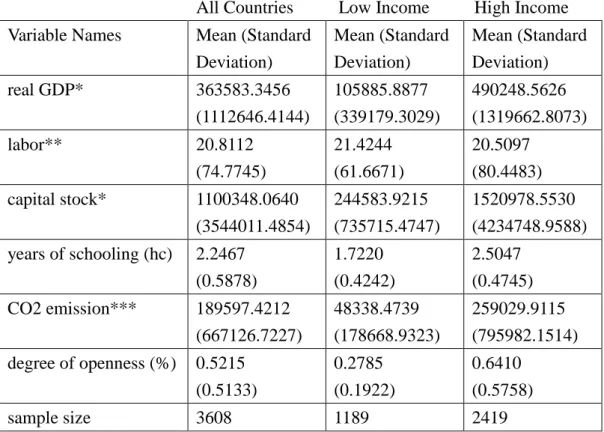
observations. The balanced panel data consist of 88 countries spanning 41 years. We further classify our sample countries into two groups, i.e., low income (29 nations) and high income (59 nations) groups.8 Table 1 presents descriptive statistics. Table 1 shows that the average GDP of the high income group is around four times as large as that of the low income group, where the former employ much larger capital stock and higher quality of labor (years of schooling) than the latter, along with higher degree of openness. However, high income countries produce much larger amount of Co2 than low income countries.

IV.

Empirical Results

4.1 Group Frontiers

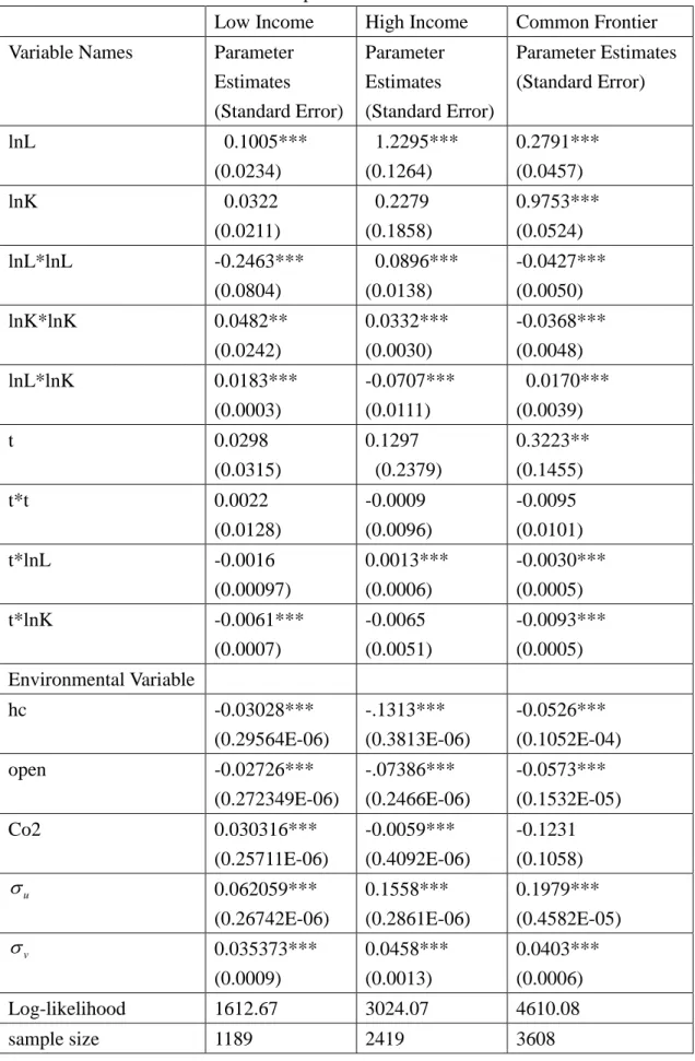
We estimate the group-specific production frontier of (1) using the likelihood function of (4) and compute technical efficiency according to (7) for each countries. Table 2 presents parameter estimates of the two groups in the first two columns and the last column shows parameter estimates of the common frontier that is yielded by estimating the pooled data of the two groups under (4). It is noteworthy that the appropriateness of the common frontier relies on the assumption that the two groups of countries adopt the same production technology, which appears to be incorrect.

8 _{The World Bank classifies countries into four groups according to the per capita GNI in 2013,}

calculated using the World Bank Atlas method, i.e., low-income economies ($1,045 or less), lower-middle-income (more than $1,045 but less than $4,125), upper-middle-income (more than $4,125 but less than $12,746), and high-income economies ($12,746 or more). The first two groups of countries are defined as our low income group and the latter two groups of countries are defined as our high income group.

14

Table 1. Descriptive Statistics

All Countries Low Income High Income

Variable Names Mean (Standard

Deviation) Mean (Standard Deviation) Mean (Standard Deviation) real GDP* 363583.3456 (1112646.4144) 105885.8877 (339179.3029) 490248.5626 (1319662.8073) labor** 20.8112 (74.7745) 21.4244 (61.6671) 20.5097 (80.4483) capital stock* 1100348.0640 (3544011.4854) 244583.9215 (735715.4747) 1520978.5530 (4234748.9588) years of schooling (hc) 2.2467 (0.5878) 1.7220 (0.4242) 2.5047 (0.4745) CO2 emission*** 189597.4212 (667126.7227) 48338.4739 (178668.9323) 259029.9115 (795982.1514) degree of openness (%) 0.5215 (0.5133) 0.2785 (0.1922) 0.6410 (0.5758) sample size 3608 1189 2419

Note: *: measured by millions of 2005 U.S$. **: measured by million persons. ***: measured by kilotons.

Most of the coefficient estimates in Table 2 attain at least the 5% level of significance. Among them, the estimates of _u is positive and significant in those three models, implying that the production efficiency be considered. The omission of it may results in inconsistent parameter estimates. A country with higher quality of labor, i.e., a higher hc value, tends to have higher technical efficiency, since its coefficient estimates are significantly negative. A higher degree of openness

stimulates a country’s production efficiency, due possibly to the fact that the country may have more opportunities to import and mimic foreign countries’ production technology and managerial ability. A high income country emits more Co2 tends to be more efficient. This may be arisen from the fact that the more emission of Co2 by a country, the less likely it employ resources to dispose Co2. The reverse is true for low income countries, which may be ascribable to the fact that the production

technologies adopted by those countries are not so advanced as to produce more Co2 emission.

To confirm that these two groups of countries undertake different technology we estimate a common frontier using the pooled data of them and the parameter estimates are show in the last column of Table 2. The likelihood ratio test statistic for the null

15

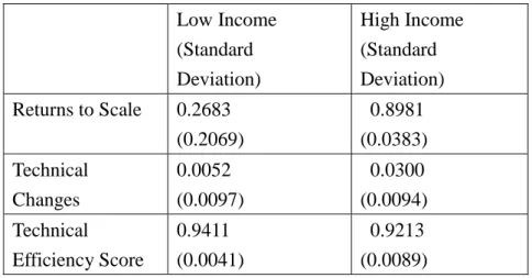
hypothesis that the two groups of countries assume the same technology is equal to 53.12, which is decisively rejected at the 1% level of significance with the degrees of freedom 14. These parameter estimates can be used to compute measures of technical changes, returns to scale, and technical efficiency score, and the results are shown in Table 3.

Both groups of countries are producing with increasing returns to scale

technology, but a representative high income country is closer to the stage of constant returns to scale due to its measure of returns to scale is greater than that of low

income countries. Moreover, the average speed of technical advance of high income countries is much quicker than that of low income countries. This is anticipated, since the labor quality of high income countries is higher, which support the use of more complicated capital invested by firms. In addition, high income countries usually involve in more R&D expenditure, which is the main source of enhancing technology. Conversely, the average technical efficiency score of low income countries is slightly greater than that of high income countries.

4.2 The Meta-production Frontier

In the second stage, we pool both groups of countries and replace their observed output (real GDP) by the fitted counterparts, obtained from the first stage. Table 4 presents parameter estimates of the meta-production frontier. Vast majority of the parameter estimates are significant at the 1% level. Following Kumbhakar (1990), we specify the inefficiency term of M

jit

 in (12) as:



2



1 exp

M M M M M

jit Vjit Ujit Vjit t t ujit

     _   _

where M jit

u is a half-normal random variable. We next apply these estimates with (14)

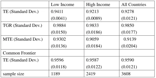
to calculate the measure of TGR. Table 5 summarizes various efficiency estimates of different groups. Both groups tend to undertake similar technology since their average TGRs are quite close to each other. The overall efficiency measures, MTE, of low and high income countries are 0.9302 and 0.9059, respectively. Low income countries are producing a little more technically efficient.

16

Table 2. Parameter Estimates of Group and Common Frontiers

Low Income High Income Common Frontier

Variable Names Parameter

Estimates (Standard Error) Parameter Estimates (Standard Error) Parameter Estimates (Standard Error) lnL 0.1005*** (0.0234) 1.2295*** (0.1264) 0.2791*** (0.0457) lnK 0.0322 (0.0211) 0.2279 (0.1858) 0.9753*** (0.0524) lnL*lnL -0.2463*** (0.0804) 0.0896*** (0.0138) -0.0427*** (0.0050) lnK*lnK 0.0482** (0.0242) 0.0332*** (0.0030) -0.0368*** (0.0048) lnL*lnK 0.0183*** (0.0003) -0.0707*** (0.0111) 0.0170*** (0.0039) t 0.0298 (0.0315) 0.1297 (0.2379) 0.3223** (0.1455) t*t 0.0022 (0.0128) -0.0009 (0.0096) -0.0095 (0.0101) t*lnL -0.0016 (0.00097) 0.0013*** (0.0006) -0.0030*** (0.0005) t*lnK -0.0061*** (0.0007) -0.0065 (0.0051) -0.0093*** (0.0005) Environmental Variable hc -0.03028*** (0.29564E-06) -.1313*** (0.3813E-06) -0.0526*** (0.1052E-04) open -0.02726*** (0.272349E-06) -.07386*** (0.2466E-06) -0.0573*** (0.1532E-05) Co2 0.030316*** (0.25711E-06) -0.0059*** (0.4092E-06) -0.1231 (0.1058) u  0.062059*** (0.26742E-06) 0.1558*** (0.2861E-06) 0.1979*** (0.4582E-05) v  0.035373*** (0.0009) 0.0458*** (0.0013) 0.0403*** (0.0006) Log-likelihood 1612.67 3024.07 4610.08 sample size 1189 2419 3608

Note: *: Significant at the 10% level. **: Significant at the 5% level. ***: Significant at the 1% level.

17

Table 3. Measures of returns to scale and technical changes Low Income (Standard Deviation) High Income (Standard Deviation) Returns to Scale 0.2683 (0.2069) 0.8981 (0.0383) Technical Changes 0.0052 (0.0097) 0.0300 (0.0094) Technical Efficiency Score 0.9411 (0.0041) 0.9213 (0.0089)

Table 4. Parameter Estimates of the Meta-Frontier

Variable Names Parameter

Estimates Standard Error lnL 0.0384*** 0.0074 lnK 0.0625*** 0.0084 lnL*lnL -0.0537*** 0.0054 lnK*lnK 0.0337*** 0.0052 lnL*lnK 0.0286*** 0.0046 t -0.0260 0.0165 t*t 0.0029*** 0.0009 t*lnL 0.00056*** 0.00009 t*lnK -0.0023*** 0.00009 Environmental Variable t 0.0845*** 0.0258 t*t 0.0054 0.0042 u  0.1506*** 0.0625 v  0.0065*** 0.00002 Log-likelihood 9598.45 sample size 3608

Note: *: Significant at the 10% level. **: Significant at the 5% level. ***: Significant at the 1% level.

18

Table 5. Various Efficiency Measures

Low Income High Income All Countries

TE (Standard Dev.) 0.9411 (0.0041) 0.9213 (0.0089) 0.9278 (0.0121) TGR (Standard Dev.) 0.9884 (0.0150) 0.9833 (0.0186) 0.9850 (0.0177) MTE (Standard Dev.) 0.9302

(0.0136) 0.9059 (0.0184) 0.9139 (0.0204) Common Frontier TE (Standard Dev.) 0.9596 (0.0118) 0.9587 (0.0122) 0.9590 (0.0121) sample size 1189 2419 3608

V.

Conclusion

This paper employs the newly developed meta-production frontier by Huang et

al. (2014) to compare technical efficiency scores for the low and high income countries, in addition to the consideration of the common effects. The stochastic

frontier model with the common effects, proposed by Hsu et al. (2013), is exploited by this paper to estimate the macro-production frontier, using country-level data. The

low and high income countries are found to utilize different production technologies and to take the increasing returns to scale technology, but the latter countries are

closer to the constant returns to scale. The speed of technical advance for high income countries is faster than that of low income countries. However, the overall technical

efficiency score of low income countries is greater than that of high income countries, due mainly to technical efficiency rather than TGR, while the difference between the

19

References

Aigner, D.J. C.A.K. Lovell and P. Schmidt (1977), Formulation and estimation of stochastic frontier production function models, Journal of Econometrics, 6, 21-37.

Ahn, S. G., Y. H. Lee, and P. Schmidt (2006), Panel data models with multiple time-varying effects, Mimeo, Arizona State University.

Ahn, S. G., Y. H. Lee, and P. Schmidt (2007), Stochastic frontier models with multiple time-varying individual effects, Journal of Productivity Analysis, 27, 1-12.

Bai, J. (2009), Panel data models with interactive fixed effects, Econometrica, 77, 1229-1279.

Battese, G.E. and J. Coelli (1988), Prediction of firm-level technical efficiencies with a generalized frontier production function and panel data, Journal of

Econometrics, 38, 387-399.

Battese, G.E., D. S. Prasada Rao, and C.J. O'Donnell (2004), A metafrontier

production function for estimation of technical efficiencies and technology gaps for firms operating under different technologies, Journal of Productivity Analysis, 21, 91-103.

Cornwell, C., P. Schmidt, and R.C. Sickles (1990), Production frontiers with cross-sectional and time-series variation in efficiency levels, Journal of

Econometrics, 46, 185-200.

Färe, R. and S. Grosskopf (2005), New directions: efficiency and productivity. Kluwer Academic Publishers, Boston, U.S.A.

Greene, W (2005b), Reconsidering heterogeneity in panel data estimators of the stochastic frontier model. Journal of Econometrics 126, 269-303.

Harville, D.A. (1997), Matix Algebra From a Statistician’s Perspective. New York: Springer.

Hsu, C.C., C.C. Lin, and S.Y. Yin (2012), Estimation of a panel stochastic frontier model with unobserved common shocks, manuscript.

Huang, C.J., T.H. Huang, and N.H. Liu (2014), A new approach to estimating the metafrontier production function based on a stochastic frontier framework, manuscript.

Inklaar, R. and M.P. Timmer (2013), Capital, labor and TFP in PWT8.0, mimeo, see

www.ggdc.net/pwt.

Johnston, J. and J. DiNardo (1992), Econometric Methods, fourth edition, McGraw-Hill companies, Inc., New York.

20

models, Sankhya, 30, 267-280.

Kumbhakar, S.C. (1990), Production frontiers, panel data, and time-varying technical inefficiency, Journal of Econometrics, 46, 201-212.

Lee, Y.H. and P. Schmidt (1993), A production frontier model with flexible temporal variation in technical inefficiency, in H.O. Fried, C.A.K. Lovell, and S.S.

Schmidt, eds, The Measurement of Productive Efficiency: Techniques and

Applications. New York: Oxford University Press.

Levinsohn, J. and A. Petrin (2003), Estimating production functions using inputs to control for unobservables, Review of Economic Studies, 70, 317-341.

Meeusen, W., and J. Van Den Broeck (1977), Efficiency estimation from Cobb-Douglas production functions with composed error, International

Economic Review, 18, 435-444.

O’Donnell, C.J., D. S. Prasada Rao, G.E. Battese (2008), Metafrontier frameworks for the study of firm-level efficiencies and technology ratios, Empirical Economics, 34, 231–255.

Olley, S. and A. Pakes (1996), The dynamics of productivity in the

telecommunications equipment industry, Econometrica, 64, 1263-1298.

Pesaran, M. H. (2006), Estimation and inference in large heterogeneous panels with a multifactor error structure, Econometrica, 74, 967-1012.

Pesaran, M. H. (2011), Panels with non-stationary multifactor error structures,

Journal of Econometrics, 160, 326-348.

Schmidt, P. and R.C. Sickles (1984), Production frontiers and panel data, Journal of

Business and Economic Statistics, 2, 367-374.

Wang, H.J. and C.W. Ho (2010), Estimating fixed-effect panel stochastic frontier models by model transformation, Journal of Econometrics, 157, 286-296.

Wang, H. J. and P. Schmidt (2002), One-step and two-step estimation of the effects of exogenous variables on technical efficiency levels, Journal of Productivity

科技部補助計畫衍生研發成果推廣資料表

日期:2014/10/15

科技部補助計畫

計畫名稱: 運用考慮交互效果的真實固定效果模型探討各國總體生產效率 計畫主持人: 黃台心 計畫編號: 102-2410-H-004-009- 學門領域: 產業組織與政策

無研發成果推廣資料

102 年度專題研究計畫研究成果彙整表

計畫主持人：黃台心 計畫編號： 102-2410-H-004-009-計畫名稱：運用考慮交互效果的真實固定效果模型探討各國總體生產效率 量化 成果項目 實際已達成 數（被接受 或已發表） 預期總達成 數(含實際已 達成數) 本計畫實 際貢獻百 分比 單位 備 註 （ 質 化 說 明：如 數 個 計 畫 共 同 成 果、成 果 列 為 該 期 刊 之 封 面 故 事 ... 等） 期刊論文 0 0 100% 研究報告/技術報告 1 1 100% 研討會論文 0 0 100% 篇 論文著作 專書 0 0 100% 申請中件數 0 0 100% 專利 已獲得件數 0 0 100% 件 件數 0 0 100% 件 技術移轉 權利金 0 0 100% 千元 碩士生 0 0 100% 博士生 0 0 100% 博士後研究員 0 0 100% 國內 參與計畫人力 （本國籍） 專任助理 1 1 100% 人次 期刊論文 0 0 100% 研究報告/技術報告 0 0 100% 研討會論文 0 0 100% 篇 論文著作 專書 0 0 100% 章/本 申請中件數 0 0 100% 專利 已獲得件數 0 0 100% 件 件數 0 0 100% 件 技術移轉 權利金 0 0 100% 千元 碩士生 0 0 100% 博士生 0 0 100% 博士後研究員 0 0 100% 國外 參與計畫人力 （外國籍） 專任助理 0 0 100% 人次

其他成果

(

無法以量化表達之成 果如辦理學術活動、獲 得獎項、重要國際合 作、研究成果國際影響 力及其他協助產業技 術發展之具體效益事 項等，請以文字敘述填 列。) 無 成果項目 量化 名稱或內容性質簡述 測驗工具(含質性與量性) 0 課程/模組 0 電腦及網路系統或工具 0 教材 0 舉辦之活動/競賽 0 研討會/工作坊 0 電子報、網站 0 科 教 處 計 畫 加 填 項 目 計畫成果推廣之參與（閱聽）人數 0

科技部補助專題研究計畫成果報告自評表

請就研究內容與原計畫相符程度、達成預期目標情況、研究成果之學術或應用價

值（簡要敘述成果所代表之意義、價值、影響或進一步發展之可能性）

、是否適

合在學術期刊發表或申請專利、主要發現或其他有關價值等，作一綜合評估。

1. 請就研究內容與原計畫相符程度、達成預期目標情況作一綜合評估

■達成目標

□未達成目標（請說明，以 100 字為限）

□實驗失敗

□因故實驗中斷

□其他原因

說明：

2. 研究成果在學術期刊發表或申請專利等情形：

論文：□已發表 □未發表之文稿 ■撰寫中 □無

專利：□已獲得 □申請中 ■無

技轉：□已技轉 □洽談中 ■無

其他：（以 100 字為限）

3. 請依學術成就、技術創新、社會影響等方面，評估研究成果之學術或應用價

值（簡要敘述成果所代表之意義、價值、影響或進一步發展之可能性）（以

500 字為限）

過去利用隨機邊界模型探討個體廠商或總體生產效率的研究，大多未將無法

觀察到的共同衝擊因子 (unobserved common shocks) 納入考量。本研究運用

Greene (2005a, 2005b) and Wang and Ho (2010) 真實固定效果模型搭配 Hsu

et al. (2012) 發展的方法，利用 Pesaran (2006) 的方法先對迴歸模型進行轉

換，設法消除交互與固定效果，再針對轉換後模型以最大概似法進行估計各

國總體隨機生產邊界函數，就可得到具備一致性的係數與效率估計值。進一

步將樣本國家分成已開發和開發中兩群組或更多群組，採用 Huang et al.

(2012) 發展的新共同生產邊界模型進行生產效率與生產力之比較。

將這種無法觀察到的共同衝擊因子納入迴歸模型，表示各國生產活動具

有橫斷面相依性與來自共同因子的異質衝擊。迴歸模型若忽略這種交互效

果，易造成係數與效率估計值的偏誤。

本研究嘗試發展新的計量方法，解決上述問題，為伴隨而生者，概似函

數的非線性問題導致迴歸係數極不容易估計。在結案時間限制之下，目前僅

無法進行比較，但預期應有很大差異。研究成果具有實證應用價值，經改寫

後可投稿至國外學術性期刊，具有發表之潛力。