多變數程序之控制策略及控制系統設計

行政院國家科學委員會專題研究計畫 成果報告

多變數程序之控制策略及控制系統設計

研究成果報告(精簡版)

計 畫 類 別 ： 個別型

計 畫 編 號 ： NSC 95-2221-E-002-378-

執 行 期 間 ： 95 年 08 月 01 日至 96 年 10 月 31 日

執 行 單 位 ： 國立臺灣大學化學工程學系暨研究所

計 畫 主 持 人 ： 黃孝平

計畫參與人員： 博士班研究生-兼任助理：林峰毅

博士後研究：鄭智成

處 理 方 式 ： 本計畫可公開查詢

中 華 民 國 96 年 11 月 27 日

行政院國家科學委員會補助專題研究計畫

■ 成 果 報 告

□期中進度報告

多變數程序之控制策略及控制系統設計

計畫類別：▓ 個別型計畫 □ 整合型計畫

計畫編號：NSC 95－2221－E －002－378－

執行期間：

95 年 8 月 1 日至 96 年 10 月 31 日

計畫主持人： 黃孝平 教授

共同主持人：

計畫參與人員： 林峰毅、鄭智成

成果報告類型(依經費核定清單規定繳交)：▓精簡報告 □完整報告

本成果報告包括以下應繳交之附件：

□赴國外出差或研習心得報告一份

□赴大陸地區出差或研習心得報告一份

□出席國際學術會議心得報告及發表之論文各一份

□國際合作研究計畫國外研究報告書一份

處理方式：除產學合作研究計畫、提升產業技術及人才培育研究計畫、

列管計畫及下列情形者外，得立即公開查詢

□涉及專利或其他智慧財產權，□一年□二年後可公開查詢

執行單位：國立台灣大學化工系

多變數程序之控制策略及控制系統設計

計畫編號：NSC 95－2221－E －002－378－

執行期間：95 年 8 月 1 日至 96 年 10 月 31 日

Abstract: In this project, a systematic procedure is proposed for the generalized design of decoupling multivariable controller, which may result in a complete decoupling, partial decoupling or no decoupling, to achieve a better disturbance rejection response. Before the decoupling, a relative load gain (abbr. RLG) is defined to determine which control loops need to be decoupled and which control loops don’t. By a transitional design matrix and its adjoint matrix, a completely or partially inverse-based multi-input-multi-output (MIMO) decoupler with generalized form is presented to decouple the process into the specified open-loop process. This decoupled open-loop process is further decomposed into several equivalent single-loop systems, equivalent open-single-loop processes and disturbances. Finally, the controller can be synthesized based on each equivalent system for disturbance rejection. Stability robustness of the system is tuned with measures for the modeling errors in the decoupled open-loop process. Simulation examples are illustrated to show that this proposed method is effective for disturbance rejection in MIMO systems.

1. INTRODUCTION

Most chemical plants belong to multi-input-multi-output (MIMO) processes having multiple delays. The main characteristic of MIMO process is interaction existence between loops and that leads to difficult use for the conventional SISO controllers. Because of this, many methods have been developed to construct multivariable control systems. Lots of them intend to make the system strictly or roughly dominated by diagonal elements or to reduce the effect from loop interactions. In general, these multivariable controllers are considered to have better control ability than multi-loop SISO controllers. However, Niederlinski (1971) reveals that multiloop SISO controllers may give better load rejection than inverse-based multivariable controllers for some cases. To analyze differences of load responses between multi-loop SISO controllers and inverse-based multivariable controllers, Stanley et al. (1985) proposed the relative disturbance gain (RDG) which is defined as a ratio of the manipulated variable under perfect control at steady-state and single-loop control. Actually, the control structure that has superior ability for disturbance rejection may be neither the multi-loop SISO controller nor inverse-based multivariable controller (Chang and Yu, 1992; Fragervik et al., 1983). It can be any structure, for example, partial decoupling, that is a structure between two extreme cases. Some forms of partial decoupling have been proposed such as block diagonal decoupling (Linneman and Wang, 1993) and triangular decoupling (Gómez and Goodwin, 2000). Most of them only discuss the delay-free systems which seldom exist in chemical processes. Although some one-way decoupling methods (Fragervik et al., 1983; Arkun et al., 1984) can be easily applied to TITO systems having multiple delays, they are difficult to extend to higher dimensional systems. Besides, most methods only pick on

one control structure and lack a criterion to select a proper structure.

In this project, a systematic procedure is proposed to design the multivariable controller with generalized form to perform well disturbance rejection. A relative load gain (RLG) is defined to determine the decoupling structure even for the partial decoupling case. Moreover, RLG has explicit physical meaning and direct connection to control performance. A method is proposed to design the generalized decoupling that could be a complete decoupling, partial decoupling or non-decoupling. Furthermore, measures of modeling error are given to facilitate the analysis of system robustness.

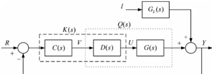
2. GENERALIZED DESIGN OF DECOUPLING A multivariable control scheme with unity feedback loop is shown in Fig. 1. To control this MIMO system, two common methods are usually used. One is the complete decoupling (i.e. the inverse-based multivariable control) that results a fully controller K s and inverse-based decoupler ( ) D s . ( ) The other is non-decoupling (i.e. the decentralized control) that brings ( )K s decentralized and ( )D s identity. Consider

a n n´ system as the following:

( ) ( ) ( ) L( ) ( )

Y s =G s U s +G s l s (1)

where, Y s and ( ) U s designate the output and input ( ) vectors, ( )l s and G s represent the load and its transfer _L( ) function vector (abbr. TFV), and ( )G s is the process transfer

function matrix (abbr. TFM). Both G s and ( ) G s are _L( ) open-loop stable. The objective of generalized decoupling is to remove loop interactions in some loops but to remain them

Fig. 1. A multivariable control scheme with unit feedback

in the other loops. First, ( )G s is factorized into two parts:

( )

( )

( )

( )

1 11 1 1 0 0 ( ) 0 0 0 0 ( ) ( ) n s o o n s on onn o e g s g s G s e g s g s s G s q q -= = Q é ù é ù ê ú ê ú ê ú ê ú ê ú ê_ë ú_û ë û L O M O M L (2)

where qi =min

{

q qi1, i2, ,Lqin

}

. For explicit explanation,

( )

o

G s is permuted to the following form, that is:

11 12 11 12 need to be decoupled

do not need to be decoupled

21 22 21 22 o o o o o o o o o G G G G G G G G G = = é ù é ù ê ú ê ú ê ú ê ú ê ú ê ú ë û ë û M LLLL LLLL LLLLLL M (3) where 11 m m o G _ÎR ´ _, ( ) 12 m n m o G _ÎR ´ - _, ( ) 21 n m m o G _ÎR - ´ _{, and} ( ) ( ) 22 n m n m o

G _ÎR - ´ - _{. The upper m loops need to be decoupled}

but the other loops do not. Define a transitional design matrix:

( ) ( ) ( ) 11 12 o o n m m n m n m G G A O _{- ´} I _{- ´} -= é ù ê ú ê ú ê ú ë û M LLLLLLLLL M (4)

where I₍n m- _{) (}´ -n m₎ is an identity matrix with dimension

(

n m-

) (

´ n m-

)

and O₍n m- ₎´m is a zero matrix with

dimension

(

n m-

)

´m. The dynamics of the upper part of

( ) o

G s are preserved in A s( ) in order to decouple these loops. In the non-decoupling part, A s( ) is designed by

(n m) (n m)

I _{- ´ -} and O_{(n m- )´m} instead of G and _o21 G . Based on _o22

the design matrix A s( ), an effective design of decoupler is proposed as the following:

{ }

{ }

( ) ( ) ( )

{ }

{ }

{ }

( )

{ }

( ) ( ) 1 1 1 11 11 12 11 11 11 12 11 adj det det adj adj det o o o o n m m n m n m o o o o n m m n m n m D A Z A A Z G G G G Z O I G G G Z O G I -- -- ´ - ´ -- ´ - ´ -= = -= -= é ù ê ú ë û é ù ê ú ë û (5) where ( ) diag{ ( )} i Z s = z s , adj{ ( )}

[

ji( ); , 1, ...,

]

A s = A s i j= n , and ( ) ij

A s is the cofactor of a s_ij( ). Notice that each diagonal element z s_i( ) is given as a simple and stable transfer function. The decoupler are open-loop stable, since G s( ) is open-loop stable, as has been mentioned. Then, the decoupled open-loop process ( )Q s is given as:

{ }

( )

{ }

{

}

{ }

{ }

( )

{ }

{ }

{ }

11 -1 1 21 11 11 22 21 11 12 11 11 21 11 22 11 21 11 12 11 12 21 22 det det det det

adj det adj

o m m o m n m o o o o o o o o m m o m n m o o o o o o o o o o o Q G D I G O Z G G G G G G G G I G O Z G G G G G G G Q Q Q Q ´ ´ -´ ´ -= Q = Q -= Q -= Q

é

ù

ê

ú

ë

û

é

ù

ê

ú

ë

û

é

ù

ê

ú

ë

û

(6)

From (6), the partial decoupling is obtained and ( )Q s are

open-loop stable. When A s( ) is specified as the entire matrix of G s_o( ), (6) results the complete decoupling that is

{ }

det _o

Q= Q G Z. So, the above derivations show that the proposed method can generate either the partial decoupling or complete decoupling.

3. GENERALIZED MULTIVARIABLE CONTROLLER DESIGN

A generalized multivariable controller ( )K s can be regarded

as combination of a decentralized controller C s( ) and a generalized decoupler D s( ), as shown in Fig. 1. As the mention of generalized decoupling, a criterion for control structure selection is needed to specify the design matrix first to design the decoupler in (5).

3.1 Control Structure Selection

The effect of load change can be suppressed or amplified via process interactions. If interactions amplify the load, the decoupling control may be required. On the other hand, interactions favour the system for load rejection. Therefore, a measure for evaluation the controller structure vs. disturbance rejection capability is desirable. Here, a relative load gain (RLG) is defined as the following

all loops except closed

all loops open

i i i i y l y l g ¶ ¶ = ¶ ¶ æ ö ç ÷ è ø æ ö ç ÷ è ø (7)

Notice that, theoretically, errors caused by the disturbances can only be eliminated after a dead-time period so the error

magnitude in the output is proportional to the load gain of the system during this period. Thus, RLG is closely linked to the control performance. From the definition in (7), RLG can be computed as: (0) (0) Li Li i Li Li g k g k g = = (8)

where k and _Li k are the gains of _Li g s and _Li( ) g s , _Li( ) respectively. g s is defined as the effective disturbance _Li( ) that means the total effect of load input to the ith loop when all loops except i are closed. In order to derive the g s , the _Li( ) matrices in (1) are first permuted and partitioned into the following forms: ( ) ( ) 12 ( ) ( ) 21 22 i i ii i i g G G G G =

é

_ê

ù

_ú

ë

û

; ( ) ( ) 2 0 ; 0 Ci i C i C g G G =

é

_ê

ù

_ú

ë

û

( ) ( ) 2 Li i L i L g G G =

é

_ê

ù

_ú

ë

û

(9)

Then, the effective disturbance of the ith loop is given as:

(

)

{

}

1 1 ( ) ( ) ( ) ( ) ( ) 12 22 22 2 2 i i i i i Li Li C L g = g -G

é

_ë

G

ù

_û

- I- I G G+ - G (10)

The RLG can be applied to determine that the loop favours to be decoupled or not. Furthermore, the outputs that have their absolute value of g_i more than one can be suggested to be decoupled so MISO controllers are used here. On the other hand, g_i £1, these loops favour to use SISO controllers. The selection of controllers can be based on the following criterion:

1; MISO controller is preferred for 1; SISO controller is preferred for

i i i i y y g g > £

ì

í

î

Notice that, if both SISO and MISO controller are needed in an MIMO process, the controller needed will be a partial decoupling controller.

3.2 Design of D s( )

According to the RLG in (7), the design matrix can be specified by the following criteria:

{

}

{

}

, , , , ( ) ( ) 1 ( ) ( ) ( ) 1 i oi i i i i A s G s i i A s A s I s i i g g · · · · = " Î > = = " Î £ ì í î (11)

where A s_i,·( ), G_oi,·( )s , and I_i,·( )s designate the ith rows of A s( ), G s_o( ), and a unit matrix I , respectively. To implement D s( ) of (5), each ij( )

A s is reduced to a simpler transfer function, that is,

(

)

(

) (

)

, 1 2 ,1 ,2 , 1 1 ˆ ( ) ( ) 1 1 n A s A r i ij i ji p A A A p p g i i k e s s A s s s s d _t f t t t -= = + = = + + +

Õ

Õ

(12)

where n and p are the number of first order leads and lags respectively and they obey the inequality of p+ - >2 n 0. The parameters in the model of (12) can be obtained by solving the following optimization problem:

( )

( )

2 0 ˆ arg min f ij ij A j A j d w w w w =

ò

-P P (13) where =[ , A_,, A_,, A_,1, and A_,2] g i r i p p d t t t t P , w_f is a frequency band which is chosen as ten times frequency bandwidth of _{A s}ij( )

. In order to make each element of D s( ) realizable, a number of excess zeros of z s_i( ) is given as the following:

{

}

[ ( )] min [ ( )], 1, 2,..., ez ep i ji N z s = N f s j= n (14) where ep[ ( )] ji

N f s is the number of excess poles in f_ji( )s . From (6), the dynamics of decoupled parts in Q s( ) are dominated by det

{ }

G_o11 . According to that, the decoupled loop in the proposed design can be obtained by a simpler expression as the following:

{

}

1 ( ) 1 n ij ij i j w s g A i i g = =

å

" Î > (15) ( )

w s can be implemented by a reduced order form of the following,

(

)

(

) (

)

, 1 2 ,1 , 2 , 1 1 ( ) ( ) 1 1 ex ex n s D D r i s o i p D D D p p g i i k e s s s e s s s q q t j j t t t -= = + = = + + +

Õ

Õ

(16)

Similarly, the parameters in (16) can be obtained by solving the optimization problem as in (13) except that j( )s and

( )

w s are instead of Aˆij and ij( )

A s . w_f is chosen as ten times frequency bandwidth of w s( ). Then, by re-allocate the pole(s) and zero(s) in j( )s , z s_i( ) provides the availability to modify undesirable dynamic characteristics in w s( ), and thus can improve the dynamics resulting from some large time constants or excessive lags. The decoupler D s( ) is thus implemented via the transfer functions of the following:

ˆ

( ) ( ) ( ) ji( ) ( ), ,

ij ij j j

An index is defined to indicate the effectiveness of decoupling,

( )

( )

( )

(

, ˆ max ji ji 0, ji g i ii q j q j q j w w w e w w w -= " Î _ùû (18) where 1 n ik ji jk i k q g A z = =

å

, 1 1 ˆ ˆ n n ik ji jk ki i jk i k k q g f z g A z = = =

å

=

å

, and , g i

w is the frequency bandwidth of q s_ii( ). The index in (18) means the relative discrepancy between q s_ji( ) and q sˆ ( )_ji . If this value is too large to be not satisfactory, the model orders of f( )s need to be increased. In other words, e_ji serves as a tuning factor to improve the stability robustness of the system. For good stability robustness, it is recommended that e_ji is less than 0.1.

3.3 Design of C s( )

As the multivariable control scheme in Fig. 1, after the decoupling, a decentralized controller C s( ) is designed for a new open-loop process ( )Q s that is presented as the dotted

block in Fig. 1. For an inverse-based multivariable controller or a multivariable controller with complete decoupling, the process is decoupled into several individual open-loop processes q s_ii( ) so the design of each decentralized controller c s_i( ) can be simplified as the design in single-loop system with each open-single-loop process q s_i( ). However, the generalized decoupling may give partial results of complete decoupling as the upper part of ( )Q s in (6) and the

other results of non-decoupling as the lower part of ( )Q s in

(6). Because the generalized decoupler may produce two different kinds of open-loop processes, the design of C s( )

may suffer two design problems. In order to simplify the dual design problems to one design problem, this decoupled process is decomposed into several effective processes that have been presented in elsewhere (e.g. Huang et al., 2003). Furthermore, the effective disturbance to each effective process can be derived as in (10). The decoupled process is first found according to the proposed method, that is:

{

}

( ) ( )adj ( ) ( )

Q s =G s A s Z s (19)

Next, the matrices are permuted and partitioned into the following forms: ( ) ( ) 12 ( ) ( ) ( ) ( ) ( ) ( ) 2 2 21 22 0 ; 0 i i Li i ii i i L i i i i L c g q Q Q C G C G Q Q =é_ê ù_ú =é_ê ù_ú =é_ê ù_ú ë û ë û ë û; (20)

Then, the equivalent single-loop system for the ith loop is presented as:

{

(

)

}

(

)

{

}

1 1 ( ) ( ) ( ) ( ) ( ) , 12 22 22 2 21 1 1 ( ) ( ) ( ) ( ) ( ) , 12 22 22 2 2 i i i i i E i ii i i i i i E Li Li L q Q Q I I Q C Q g g Q Q I I Q C G q - -- -= - - + = - - + é ù ë û é ù ë û (21)

According to the simplification in Huang et al. (2003), the equivalent loop and disturbance can be rewritten to the following forms, that is

1 * ( ) ( ) ( ) *( ) , 12 22 21 1 * ( ) ( ) ( ) *( ) , 12 22 2 i i i i E i ii i i i i E Li Li L q q Q Q Q H g g Q Q G H -= - Ä = - Ä é ù ë û é ù ë û (22) where *( ) * * * * * 1 2 1 1 [ , , , , , , ] i T i i n H = h h L h_- h₊ L h and each * j h is

designed for q s_ii( ) and

g

_Li( )s . Then, the reduced models of

* , E i q and * , E Li

g can be found by fitting their frequency responses as mention earlier. After these procedures, the controller design for c s_i( ) becomes one SISO control problem. The process output in response to a load l s( ) is:

[

]

* , * , , * , ( ) ( ) ( ) 1 ( ) 1 ( ) ( ) E Li i E Li E i E i i g s y s g s h s q s c s = = -+ (23)

where h_{E i,}( )s is the equivalent complementary sensitivity function and is designed for the equivalent system. By the method of Huang and Lin (2006), h_{E i,} ( )s can be found to minimize an integral of the absolute error (IAE) at an assigned peak value of sensitivity function. Then, c s_i( ) can be synthesized by: * , , * * , , , , ( ) ( ) 1 1 ( ) ( ) 1 ( ) ( ) 1 ( ) i E i E oi i _s E i E i E oi E oi h s h s c s q s h s q s _{h s e}-q = = - _- (24) where * i

q is the delay time of * , ( ) E i q s and h_{E i,} ( )s , and, * , ( ) E oi

q s and h_{E oi,} ( )s are the delay-free part of q*_{E i,}( )s and

, ( ) E i

h s . By applying the first order Pade’s approximation for in (24), the controller c s_i( ) can be given as:

* , , * * * , , ( ) ( )(1 / 2) ( ) ( ) (1 / 2) ( )(1 / 2) f i E oi i i E oi i E oi i g s h s s c s q s s h s s q q q + = + - - (25) where f i,( ) 1

(

, 1

)

n f i

g s = t s+ and t_{f i,} is the filter time constant and has a default value as _0.05 *

i

q . Finally, the generalized multivariable controller can be obtained by:

( ) ( ) ( ) , ij ij j j

4. STABILITY AND ROBUSTNESS

Assume that m loops are decoupled in an arbitrary n n´

system, where mÎ

[

1, 2, ,_K n

]

. For convenient analysis, the loops the have been decoupled are permuted to the forehead loops of the system, hence the open-loop process ( )Q s and

the controller C s( ) are rewritten as the following:

[

]

[

]

[

]

[

]

11 21 22 ( ) 1 2 ( ) decoupling part ( ) non-decoupling part decoupling part ( ) non-decoupling part m n n m n n n m n n m n n n Q O Q s Q Q C O C s O C ´ - ´ ´ ´ - ´ ´ = = é ù ê ú ê ú ê ú ë û é ù ê ú ê ú ê ú ë û LLLLLLLL LLLLLLLLLL LLLLLLLL LLLLLLLLLL (27)

where C1=diag

[ ]

c1,ii

,

C2=diag

[ ]

c2 ,jj

,

Q11 =diag

[ ]

q11,ii

,

[ ]

21 21, ji

Q = q and Q22 =

[ ]

q22 , jj for all iÎ

[

1, 2,...,m

]

and

[

1, 2,...,

]

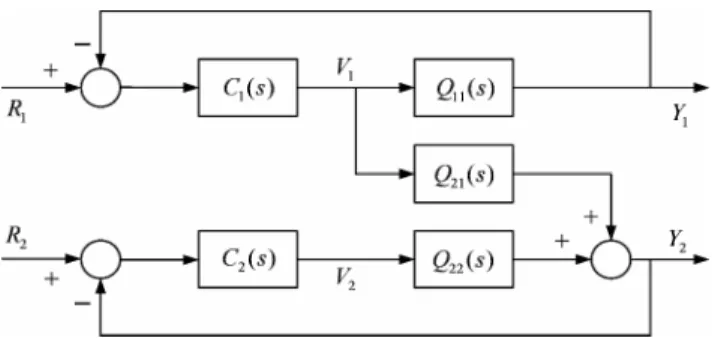
jÎ m+ m+ n . According to the proposed design, the control scheme in Fig. 1 can be regarded as an equivalent multivariable control scheme as shown in Fig. 2 that conjugates a multivariable decentralized control system with some single-loop control systems. Because each element of the process G s( ) in (1) is an open-loop stable function, the decoupled open-loop process Q s( ) in (19) and the generalized decoupler in (17) are designed to be open-loop stable. Under the conjunctive framework in Fig. 2, the stability of the system can be individually discussed by two steps: one is C s stabilizes a diagonal system 1( ) Q s and 11( )

the other is C s stabilizes a full system ₂( ) Q s . However, ₂₂( ) the approximation of D s( ) in (17) leads to the existence of modeling error in the desired process Q s . Thus, the ( ) nominal stability of the proposed control scheme in Fig. 1 is guaranteed by designing C s( ) to satisfy the following conditions:

(1) C s( ) stabilizes ( )Q s in a simple closed loop.

(a) c_1,ii( )s stabilizes q_11,ii( )s for all iÎ

[

1, 2,...,m

]

. (b) 1+c_2,ii( )s q_{22 ,E i}( ) 0s = has no RHP zero, and q_{22 ,E i}( )s

has no RHP pole for all iÎ

[

m+1,m+2,...,n

]

. (2)

[

]

{

1

}

_{

_[

1

_]

_}

( ) ( ) ( ) ; [0, ) ( ) C j I Q j C j Max Q j w s w w w w s w -- + £ " Î ¥ D

where q_{22 ,E i} is the effective process of Q₂₂, and s denotes the largest singular value.

Due to approximation made in (12), G s D s( ) ( ) may not equal to ( )Q s exactly. As a result, a model error (i.e. DQ s( )) originating from this approximation can be estimated by the index e_ij of (18) in the frequency range of concerned for nominal stability, and then the second condition can easily be

Fig. 2. An equivalent multivariable control scheme in the generalized decoupling

satisfied. As for stability robustness to modeling error of ( )

G s , consider the control system has an additive uncertain,

where the real process is presented as:

( ) ( ) ( )

G s% =G s + D s ; s( (D jw))£ _l(jw) (28) where the perturbation D( )s is bounded on _l(jw). And, the system will be robust stable iff:

[

M j( ) (

]

j ) 1,

[

0,

)

s w l w < wÎ ¥ (29) where

[

]

1 ( ) ( ) ( ) ( ) ( ) ( ) M s = -D s C s I G s D s C s+ - (30) Thus, by selecting an adequate h_{E i,}( )s , the controller c s_i( )

is synthesized also to satisfy the robust stability in (28).

5. ILLUSTRATIVE EXAMPLE

Consider the following transfer function matrix for the process and transfer function vector for load.

5 5 5 10 10 10 7 4 5 10 1 20 1 30 1 ( ) ; ( ) 4 6 4 10 1 20 1 30 1 s s s L s s s e e e s s s G s G s e e e s s s - - -- - -+ + + = = -+ + + é ù é ù ê ú ê ú ê ú ê ú ê ú ê ú ê ú ê ú ë û ë û (31)

First, the process TFM is factorized into two parts, that is:

5 10 7 4 0 _{10 1 20 1} 4 6 0 10 1 20 1 s s e _{s s} G e s s -+ + = -+ + é ù ê ú é ù ê ú ê ú ë û ê ú ê ú ë û (32)

The values of RLGs in both loops are computed by (7) as:

1 1.53

g = and g₂ =0.29. This result indicates that the first loop needs to be decoupled but the second loop does not. By (11), the transitional design matrix is given as:

1, 7 4 10 1 20 1 A s s ·= + + é ù ê ú ë û and A2,·=

[

0 1

]

Table 1. The equivalent single-loop control systems

To compute (14), a number of excess zeros of z s₁( ) and

2( )

z s are zero and one, respectively. Because the first loop obeys g_i >1 , (15) gives the following relation:

7 ( ) 10 1 w s s = + (33) Based on _{N z s}ez[ ( )] 0_{1 = and} 1 [ ( )] 1 ez N z s = , z₁ is specified as one and z s₂( ) is selected as (10s+1) to compensate the undesired pole shown in (33). By (17), the decoupler is determined as:

(

)

4 10 1 1 20 1 0 7 s D s - + = ₊ é ù ê ú ê ú ê ú ë û (34)

Then, the equivalent single-loop systems are found for the decoupled open-loop process Gadj

{ }

A Z . Their reduced

models are shown in Table 1. Then, the equivalent complementary sensitivity functions are found by the method of Huang and Lin (2006) while the peak value of sensitivity function is assigned as 1.7. Next, controllers can be synthesized by (24) and the results are further reduced to the PID form as shown in Table 1. For comparison, two extreme control systems that mean the complete-decoupling and non-decoupling are also designed by individually specifying

( )

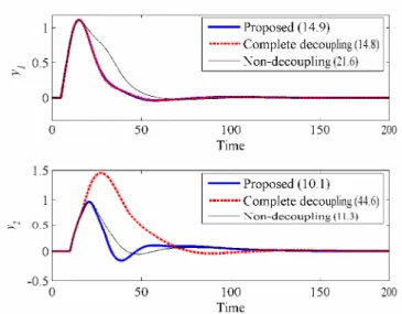
A s be G s and _o( ) I . Simulation results for a unit-step load input and their ISE values are given in Fig. 3. These results indicate that the proposed method can give the better load rejection than two conventional control methods.

6. CONCLUSION

To enhance the utility of decoupling control, a generalized design of decoupling is proposed to construct either complete or partial decoupling systems. An index of RLG is proposed to select the decoupling loops and further to determine the control structure. By a transitional design matrix, the resulting decoupler can decouple the process into the desired structure assigned by the RLG index. Then, a systematic method is proposed to construct the generalized multivariable

Fig. 3. Responses of load rejection and their ISE values controller, which can provide a suitable controller that may be the fully multivariable controller, partially multivariable controller or decentralized controller, to achieve the better disturbance response. Furthermore, this method can applied for the complex processes which have higher dimensions and multiple time delays. The stability and robustness of the system is also included to take account of modeling errors and process errors. Simulation examples have been illustrated to show that the proposed method can obtain the multivariable controller having a suitable structure and is effectiveness in disturbance rejection.

REFERENCES

Arkun Y., Manouslouthakis, B., Palazoğlu, A. (1984). Robustness Analysis of Process Control Systems. A Case Study of Decoupling Control in Distillation. Ind. Eng.

Chem. Process Des. Dev., 23, 93-101.

Chang, J. W., Yu, C. C. (1992). Relative Disturbance Gain Array. AIChE J., 4, 521-534.

Fagervik, K. C., Waller, K. V., Hammarström, L. G. (1983). Two-Way or One-Way Decoupling in Distillation? Chem.

Eng. Commun., 21, 235-249.

Gómez, G. I., Goodwin, G. C. (2000). An algebraic Approach to Decoupling in Linear Multivariable Systems. Int. J.

Control, 73, 582-599.

Huang, H. P., Jeng, J. C., Chiang, C. H., Pan, W. (2003). A Direct Method for Multi-Loop PI/PID Controller Design.

Journal of Process Control, 13, 769-786.

Huang, H. P., Lin, F. Y. (2006). Decoupling Multivariable Control with Two Degrees of Freedom. Ind. Eng. Chem.

Res., 45, 3161-3173.

Linneman, A., Wang, Q. G. (1993). Block Decoupling with Stability by Unity Output Feedback-Solution and Performance Limitations. Automatica, 29, 735-744. Niederlinski, A. (1971). Two-Variable Distillation Control:

Decouple or Not Decouple. AIChE J., 17, 1261-1263. Stanley, G., Marino-Galarraga, M., McAvoy, T. J. (1985).

Short-Cut Operability Analysis: 1. The Relative Disturbance Gain. Ind. Eng. Chem. Process Des. Dev., 24, 1181-1188. loop1 loop 2 * ,( ) E i q s 7 5 10 1 s e s -+ 10 58 20 1 s e s -+ * , ( ) E Li g s 5 5 30 1 s e s -+ 10.3 1.14 5.14 1 s e s -+ ,( ) E i h s 5 2 13.25 1 55.63 12.06 1 s s e s s -+ + + 10 1 4.67 1 s e s -+ ( ) i c s in PID form

(

)

(

)

2 135.4 18.37 1 0.0375 22.8 1 s s s s + + +

(

₍

₎

)

2 100 25 1 0.0012 1.592 1 s s s s + + -+