Learning a Scene Background
Model via Classification
Horng-Horng Lin, Student Member, IEEE, Tyng-Luh Liu, Member, IEEE, and Jen-Hui Chuang, Senior Member, IEEE
Abstract—Learning to efficiently construct a scene background
model is crucial for tracking techniques relying on background subtraction. Our proposed method is motivated by criteria leading to what a general and reasonable background model should be, and realized by a practical classification technique. Specifically, we consider a two-level approximation scheme that elegantly com-bines the bottom-up and top-down information for deriving a back-ground model in real time. The key idea of our approach is simple but effective: If a classifier can be used to determine which image blocks are part of the background, its outcomes can help to carry out appropriate blockwise updates in learning such a model. The quality of the solution is further improved by global validations of the local updates to maintain the interblock consistency. And a complete background model can then be obtained based on a mea-surement of model completion. To demonstrate the effectiveness of our method, various experimental results and comparisons are in-cluded.
Index Terms—Background modeling, boosting, classification,
tracking, SVM.
I. INTRODUCTION
V
ISUAL tracking systems using background subtraction often work by comparing the upcoming image frame with an estimated background model to differentiate moving fore-ground objects from the scene backfore-ground. Hence, the perfor-mance of such systems depends heavily on how the background information is modeled initially, and maintained thereafter. In this work, we aim to establish a learning approach to reliably es-timate a background model even when substantial object move-ments are present during the initialization stage. As illustrated in Fig. 1, the overall idea is to efficiently identify background blocks from each image frame through online classifications, and to iteratively integrate these background blocks into a com-plete model so that a tracking process can be automatically ini-tiated in real time. In developing such a progressive processing scheme for initializing a background model, some criteria are considered.• Stationary scene adaptation: It is commonly agreed that stationary scenes are considered as background. Thus, Manuscript received February 24, 2008; accepted December 01, 2008. First published February 06, 2009; current version published April 15, 2009. The associate editor coordinating the review of this manuscript and approving it for publication was Dr. Marcelo G. S. Bruno. This work was supported in part by NSC 95-2221-E-001-031-MY3 and NSC 95-2221-E-009-269.
H.-H. Lin and J.-H. Chuang are with the Department of Computer Science, National Chiao Tung University, Hsinchu 300, Taiwan (e-mail: hhlin@cs.nctu. edu.tw; jchuang@cs.nctu.edu.tw).
T.-L. Liu is with the Institute of Information Science, Academia Sinica, Nankang, Taipei, 115, Taiwan (e-mail: liutyng@iis.sinica.edu.tw).
Color versions of one or more of the figures in this paper are available online at http://ieeexplore.ieee.org.
Digital Object Identifier 10.1109/TSP.2009.2014810
in our design, when a moving object becomes stationary over a certain period of time, it will be incorporated into a background model. This would yield an initial background model accommodating the most recent statistics about the background scene, e.g., a parking car or an occluded area. • Gradual variation adaptation: The computation of a background model should take account of small variations caused by, e.g., gradual illumination changes, waving trees, and faint shadows. It allows a system to reduce the false detection rate of foreground objects.
• Model completion: Depending on object movements, the number of image frames needed in estimating an initial background could vary significantly. Hence, a measure-ment for the availability of a background model has to be defined so that the system can immediately begin to track objects upon the completion of model initialization. • Efficiency: A background model must give rise to
effi-cient online derivations to guarantee real-time tracking performance.
The first two criteria listed above manifest what kind of scene contents are considered as background. The last two ones illus-trate the design requirements of a background model initializa-tion system: it should be capable of deriving a complete back-ground model in a progressive manner and in real time.
In the proposed approach, two features will be observed. First, we utilize learning methods to identify background blocks. Rather than developing discrimination rules or models, we adopt learning approaches to construct a background block classifier. This strategy not only provides a convenient way of defining some preferred background types from image exam-ples, but also avoids complicated issues of manually setting discriminating parameters, because they can be resolved by learning from the chosen data. Second, the derived background model fulfills the four criteria. To achieve efficiency, a pro-gressive estimation scheme is developed and a fast classifier adopted. For the model completion criterion, an effective definition is given to indicate that a complete background model is obtained, and the subsequent tracking procedures can be started. Regarding the adaptation criteria, we implement a bottom-up block updating, in either a gradual or an abrupt fashion, for capturing the background variations and scene changes, respectively.
A. Related Work
Background modeling for tracking typically involves three issues: representation, initialization, and maintenance. For ex-ample, one could represent a scene background by assuming a single Gaussian distribution for each pixel, initialize the model by estimating from an image sequence, and maintain it during 1053-587X/$25.00 © 2009 IEEE
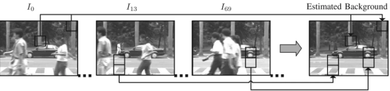
Fig. 1. Through performing online classifications and by iteratively integrating the framewise detected background blocks of images captured with a static monoc-ular camera, the scene background can be reliably estimated in real time.
tracking by updating Gaussian parameters of the background pixels. While the emphases of most previous works, including those to be described later, are mainly on representation and maintenance, the task to compute an initial background model has been somewhat neglected or otherwise simplified by not allowing large object movements throughout the initialization process, e.g., [10], [25], and [38].
1) Background Representation and Maintenance: Gaussian
models are perhaps the most popular representation for mod-eling a scene background, e.g., [4], [23], [26], [33], and [38]. Their maintenance is usually carried out in the form of temporal blending to update intensity means and variances. Thus, related researches often differ in the number of Gaussian distributions used for each pixel, and the update formulas for the Gaussian pa-rameters. In [15], Gao et al., further investigate possible errors caused by Gaussian mixture models, and then apply statistical analysis to estimate related parameters.
Apart from Gaussian assumptions, Elgammal et al. [9] con-sider kernel smoothing for a non-parametric estimate of pixel intensity over time. In [35], Toyama et al. propose a wallflower algorithm to address the problem of background representation and maintenance in three levels: pixel, region, and frame levels. Ridder et al. [30] use a Kalman-filter estimator to identify the respective pixel intensities of foreground and background from an image sequence, and to suppress false foreground pixels caused by shadow borders. In [19], a mixture of local histograms is proposed to construct a texture-based background model that is more robust to background variations, e.g., illu-mination changes.
Prior assumptions about the foreground, background, and shadows can be used to simplify the modeling complexity. For vehicle tracking, Friedman and Russell [14] propose three kinds of color models to classify pixels into road, shadow, and vehicle. They employ an incremental EM to learn a
mixture-of-Gaussian for distinguishing the foreground and
background. In [31] and [36], prior knowledge at pixel level is considered in learning the model parameters of the foreground and background. Then, a high-level process based on Markov
random field is performed to integrate the information from all
pixels.
2) Background Model Initialization: The most
straightfor-ward way to estimate a background model is to calculate the intensity mean of each pixel through an image sequence. Ap-parently, this is rarely appropriate for practical uses. Haritaoglu
et al. [17], instead, compute intensity medians over time. Yet
a more general framework by Stauffer and Grimson [33] is to use pixelwise Gaussian mixtures to model a scene background. Mittal and Huttenlocher [26] later extend the Gaussian mixture idea to construct a mosaic background model from images cap-tured using a nonstationary camera. In [35], bootstrapping for background initialization is proposed, and implemented with a pixel-level Wiener filtering.
Among the above-mentioned approaches, initializing a back-ground model is viewed more or less as part of the process for background maintenance. They do not have a systematic way to measure the quality, and determine the degree of completion for such a model. Consequently, these methods often require simple initializations, or otherwise start tracking activities with unreli-able background models.
For computing an explicit background model, Gutchess et al. [16] use optical flow information to choose the most likely time interval of stable intensity at each pixel. However, the quality of their derived background model depends critically on the ac-curacy of the pixelwise optical flow estimations. Cucchiara et
al. [6] represent a background model by pixel medians of image
samples, and specifically identify moving objects, shadows, and ghosts1for different model updates using color and motion cues.
Based on the Gaussian mixture model, Hayman and Eklundh [18] formulate a statistical scheme to derive a mosaic back-ground model with an active camera. They consider a mixel
distribution to correct the errors in background registration. In
[7], De la Torre and Black apply principal component
anal-ysis (PCA) to construct the scene background from an image
sequence. More recently, Monnet et al. [27] propose an
incre-mental PCA to progressively estimate a background model and
detect foreground changes. Still, these systems all lack an ex-plicit criterion for determining whether a background initializa-tion is completed or not—a crucial and practical element for a real-time tracking system.
Other techniques that explore layer decompositions of a video sequence can also be used to estimate a background model. Irani and Peleg [20] explore the decompositions of dominant motions and apply them to the construction of an unoccluded background image. In [12] and [21], sprite layers are derived from probabilistic mixture models, in which cues of layer ap-pearances and motions are encoded. In [1] and [2], Aguiar and Moura consider rigid motions, intensity differences, and the re-gion rigidity for figure–ground separation and formulate them as
1Ghosts are false foreground objects detected by subtracting an inaccurate
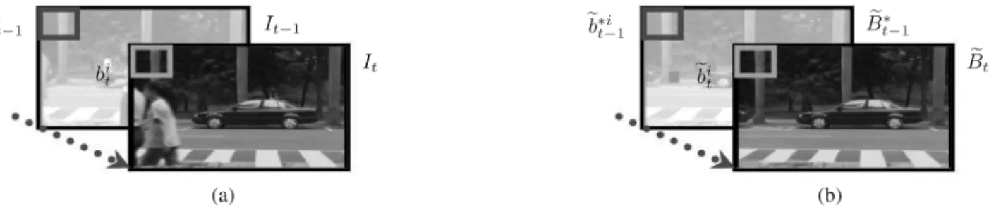
Fig. 2. (a) Online image stream:I and I are the image frames at timet and t 0 1, and their ith blocks are denoted as b and b , respectively. (b) Estimated background model: For the background models, ~B is a possible estimation at time t, while ~B is the best estimation up to timet 0 1. Accordingly, their ith blocks are represented by ~b and ~b (a) Online image stream and (b) Estimated background model.
a penalized likelihood model that can be optimized in efficient ways. In [5], [22], and [37], graph-cut-based techniques, e.g., [3], are applied to decompose video layers via pixel labeling, with various objective functions being optimized. Though all the layer-based approaches are capable of deriving a background model even for dynamic scenes, they often need to process a video sequence in batch, which is different from the proposed progressive scheme.
The rest of the paper is organized as follows. In Section II, the proposed background estimation approach is presented. In particular, the relationship between the classification and the es-timation scheme is elaborated. Then the adopted classifiers are introduced in Section III. In Section IV, some experiments are demonstrated, including training results, background estimation performance, and comparisons to other approaches. Finally, a brief discussion is given in the same section to conclude this work.
II. BACKGROUNDMODELESTIMATION VIACLASSIFICATION Due to the restriction of limited memory space and the re-quirement of real-time performance, only a small number of recent image frames are stored and referred during the con-struction of a background model. Thus, an iterative estimation scheme is proposed in the following to progressively identify background blocks in image frames and to incorporate their in-formation into a background model.
A. Iterative Estimation Scheme
To illustrate the idea of the proposed iterative estimation scheme, we begin by summarizing the notations and definitions adopted in our discussion.
• We denote the test image sequence up to time instant as , and the most recent image frames
as . We also use to stand
for the th block of , and
for the set of th blocks from (see Fig. 2).
• Let be any possible background model estimation at time , and be the estimated background model at time . Then, the th blocks of and are denoted as and , respectively.
• A training set of samples,
, is used to build a binary classi-fier, where each is a fixed-size image block
Fig. 3. Flowchart depicts the interactions between the bottom-up block updating and the top-down model validation processes. While the bottom-up process handles blockwise updates of the background, the top-down one deals with interblock consistency validations. The coupling of the two processes forms an efficient scheme for deriving a background model.
(or simply the extracted feature vector), and foreground background is its label.
• With training data , an optimal classifier can be de-fined as
(1) Equation (1) manifests that a classifier can be derived from a probabilistic maximum a posteriori (MAP) treatment [32]. It is thus more desirable to have not only classification labels/ scores but also probabilistic outputs of . In Section III, we will explain that either an SVM or a boosting-with-soft-margins classifier is appropriate for delivering such probabilities. With probabilistic outputs, a threshold can then be set to adjust the classification boundary, which is useful for our background es-timation. We will demonstrate this usage in Section IV-A-3).
The proposed iterative estimation scheme for deriving a back-ground model consists of a bottom-up block updating and a top-down model validation process. As shown in Fig. 3, a flowchart is given to illustrate the interactions between the two processes. The aim of the bottom-up process is to blockwise integrate iden-tified background blocks into a model and to form a model can-didate . Then, in the top-down process, the interblock con-sistency for all the updated background blocks are validated. By assuming that significant background updates often occur in groups, isolated updates that mainly result from noises will be eliminated by restoring their block statistics back to the previous estimates .
More specifically, in the bottom-up process, the image block classified as background and the previously estimated back-ground block act as two inputs to the background adap-tation. Based on a dissimilarity measure between the current image block and the previous background block , either a maintenance step or a replacement step is invoked for a block update. In the maintenance step, the case of the small block difference is handled, assuming it is mostly caused by gradual lighting variations or small vibrations. A new background block estimate can thus be computed by a weighted average of the two blocks and . On the other hand, when and are dissimilar, implying an occurrence of an abrupt scene change, a replacement step is employed to calculate a renewed back-ground block estimate , which is consistent with the image block .
After the above bottom-up updates, a background model can-didate is obtained. To turn this model candidate into a final estimate, a top-down process is introduced to assure the model consistency between the current candidate and the previous estimate , by assuming a smooth changing in background models. Although the checking of model consistency can be re-alized in various ways, we choose to implement it in a simple manner by finding the updates of isolated blocks and undoing them. Thus, large and grouped background block updates are preserved in this design, since they most likely belong to signif-icant and stable background changes, such as newly uncovered scenes or stationary objects. Through the validation process, a final background model estimation is derived.
It is worth mentioning that the entire approach is somehow linked to a MAP formulation, i.e.,
(2)
where is classified as a background block by
and . (Assume there are blocks in
an image frame.) Interested readers can find the derivation of (2) in the Appendix. The connections between (2) and our approach are elaborated as follows. Regarding the likelihood part, the two products can be viewed as blockwise updates after the background classification. For the image block classified as background, maximizing the probability
implies that similarities among the background estimate , the image block and the previous estimate should be retained. Likewise, for a foreground block, the corresponding probability is maximized by setting the current block estimate equal to the previous one . This is what we do in the bottom-up process. Referring to the prior term, it indicates that model level consistency between and needs to be maintained for maximizing the probability . This, as well, corresponds to the top-down
model validation. However, we note that the background model derived by our approach is only a rough approximation to the MAP solution, since (2) is not exactly solved. In fact, to optimize (2), the underlying distributions of the probability terms should be further specified, and complicated optimiza-tion techniques, e.g., EM-based estimaoptimiza-tions, may need to be employed. Hence, instead of pursuing the MAP solution, our focus is on the design of a practical and efficient algorithm for background model estimation.
B. The Algorithm
1) Bottom-Up Process: We start by applying to each to determine its probability of being a background block. A sim-plified notation will be hereafter adopted to denote such a probability, with the understanding that the most recent th-blocks s (i.e., ) are available for calculating useful features, e.g., optical flow values, for classification. Observe that only for those image blocks classified as background at each time , their corresponding blockwise updatings would modify the background model. It is therefore preferable to have as few false positives by as possible. Hence, we use a strict thresh-olding , i.e., the decision boundary of , on such
that image blocks with are considered
background. Given this setting, there are two possible cases for a block updating.
1) If is not a background block, then , i.e., the pixel means and variances of are assigned to . 2) If is classified as a background block, we measure the
dissimilarity between and by
where is the sum of squared pixel intensity dif-ferences, and is the block size. Depending on the value of , either a maintenance step or a
replace-ment step is invoked (see Algorithm 1). We apply the
iter-ative maintenance formulas proposed in [4] to update the latest small variations into . Notice that a block replace-ment in evaluating takes place only when the particular block has been classified as background for consecutive frames. Indeed, the maintenance phase is designed to adapt the gradual variations, and the replacement phase is to ac-commodate new stationary objects.
2) Top-Down Process: A top-down process based on
com-paring with is employed to detect isolated block up-dates in the bottom-up evaluation of , and undo these up-dates with the statistical data from .2Conveniently, in
im-plementing the algorithm, the top-down process can be carried out right after the background block classifications. This would yield a set of valid background blocks; all of them are not iso-lated. Hence, the bottom-up updatings over these valid blocks would directly lead to the final estimate .
2An isolated block updating (either for maintenance or for replacement)
has less than three of its 4-connected neighboring blocks being updated in the bottom-up process.
3) The Background Model: Having described our two-phase
scheme to iteratively improve , we are now in a position to define a meaningful and steady initial background model .
Definition 1: The initial background model is said to be , if is the earliest time instant satisfying the fol-lowing three conditions: i) there is no block replacement occurred for the last image frames, i.e., in calculating ; ii) all image blocks in have been replaced at least one time since ; and iii) they are of ages at least . (See Algorithm 1 for details. In all our
experiments, we have and .)
III. FASTCLASSIFICATIONWITHSOFTMARGINS In this section, issues related to the feature selection and the classifier formulation are addressed for the construction of an efficient background block classifier. In the feature selection, we have chosen to use features as general as possible so that the resulting classifier can handle a broad range of image sequences. Regarding the classifier formulation, two learning methods, support vector machines (SVMs) and column
gen-eration boost (CGBoost), are explored by investigating the
following two issues. First, rather than binary-value classifiers, a classifier with probability outputs is required for our appli-cation. Second, the efficiency of the resulting classifier should fulfill the demand of real-time performance.
A. Feature Selection
For our purpose, the task of training is to learn a binary clas-sifier for identifying background blocks from a video sequence captured by a static camera. We use a two-dimensional fea-ture vector to characterize an image block . The first com-ponent is the average optical flow value, where we apply the Lucas–Kanade’s algorithm [24] to compute the flow magnitude of each pixel in . In our implementation, it takes three image frames, , and , to calculate the flow values prop-erly. However, we note that if one-frame delay is allowed, a slightly better results in evaluating the values of optical flow can be achieved by referencing , and . The second component of a feature vector is derived from the (mean)
inter-frame image difference by .
To ensure good classification results, the feature values of both dimensions are normalized into [0,1] for training and for testing. The two feature components are discriminant enough for our application owing to their generality and consistency in classi-fying background blocks of varied image sequences. We should also point out that since the optical flow values are computed using just three consecutive image frames, it may occur that a few pixels would have erratic/large flow values. Hence, an esti-mated uppbound threshold is enforced to eliminate such er-rors. On the other hand, the additional cue using temporal dif-ferencing is more stable and easier to calculate, but it may fail to detect all the relevant cases. For example, the interframe dif-ference may not be small in evaluating a background block that consists of slightly waving trees. Instead, an optical flow value is more informative to capture such a background block with small motions.
B. SVMs With Probability Outputs
For binary classifications, SVMs determine a separating
hy-perplane by transforming from the
input space to a high dimensional feature space, through a map-ping function . The optimal hyperplane can be obtained by solving the following soft-margin optimization problem:
subject to (3)
where are slack variables for tolerating sample noises and outliers. The two parameters and are useful when dealing with unbalanced training data. (Recall that “ ” is for background image blocks and “ ” for foreground image blocks.) For the sake of reducing false positives, which may lead to more serious flaws in the estimated background model than false negatives would cause, is given a value four times larger than the one for to penalize more the mis-classifications of foreground blocks. In solving (3), we use a degree 2 polynomial kernel to yield satisfactory classification outcomes efficiently.
1) Probability Output: We use a sigmoid model to map an
SVM score into the probability of being a background block by (4)
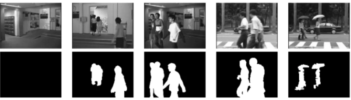
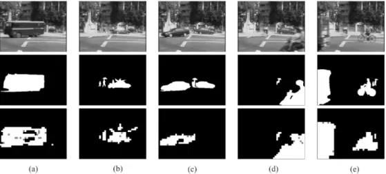
Fig. 4. Training data. Examples of collected images and their binary maps of the foreground (white) and the background regions (black) are plotted, top and bottom, respectively.
where the two parameters and can be fitted using
max-imum likelihood estimation from . Following [28], a
model-trust algorithm is applied to solve the two-parameter
optimiza-tion problem. In our experiments, 65% of the training blocks are used for deriving an SVM, and the other 35% are for cali-brating probability outputs. The two fitted parameters are
and .
C. CGBoost With Probability Outputs
Among the many variants of boosting methods, the AdaBoost, introduced by Freund and Schapire [11], is the most popular one to derive an effective ensemble classifier iteratively. While AdaBoost has been proved to asymptotically achieve a max-imum margin solution, recent studies also suggest the adoption of soft margin boosting to prevent the problem of overfitting [8], [29]. We thus employ the linear program boosting proposed by Demiriz et al. [8] for achieving soft-margin distribution over the training data and acquiring an ensemble classifier , which is comprised of weak learners s and weights s. Actually, Demiriz et al. apply a column genera-tion method to solve the linear program by part, and establish an iterative boosting process that is similar to AdaBoost. Note that in implementing the CGBoost, the weak learners are constructed from radial basis function (RBF) networks, denoted as s [29]. And each has three Gaussian hidden units where two of them are initialized for the background, and the remaining one is for
the foreground training data. Let be the
weak learner selected at the th iteration of CGBoost. Then, the RBF network is derived by minimizing the following weighted error function
(5) where is the weight distribution over training data at the
th iteration.
1) Probability Output: Different from (4), it is more
con-venient to link boosting scores to probabilities. Friedman et al. [13] have proved that the AdaBoost algorithm can be viewed as a stagewise estimation procedure for fitting an additive logistic regression model. Consequently, a logistic transfer function can be directly applied to map CGBoost scores to posterior proba-bilities by
(6)
where the mapping in (6) is valid when the training data do not contain a large portion of noisy samples or outliers. For the general case, it should still yield reasonable probability values with respect to the classification results by s.
To summarize, both the two classifiers, and , seek a soft-margin solution when deciding a decision boundary for the training data . They indeed achieve similar classification per-formance in our experiments. However, SVMs are generally less efficient than boosting, as the number of support vectors in-creases rapidly with the size of . We thus prefer a CGBoost classifier for estimating an initial background model.
IV. EXPERIMENTALRESULTS ANDDISCUSSIONS To demonstrate the effectiveness of our approach, we first de-scribe how the classifiers are learned for the specific problem. We then test the algorithm with a number of image sequences on a P4 1.8 GHz PC. Through illustrating with the experimental results, we highlight the advantages of learning a background model by classification, and make comparisons with those re-lated works. Finally, possible future extensions to the current system are also explored.
A. Classifier Learning
1) Training Data: We begin by collecting images that
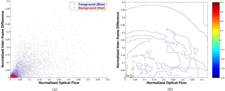
contain moving objects of different sizes and speeds from var-ious indoor and outdoor image sequences captured by a static camera. These images are analyzed using a tracking algorithm (with known background models), decomposed into 8 8 image blocks, and then manually labeled as for background blocks, or for foreground ones. Examples of the collected images and the detected foreground and background regions are shown in Fig. 4. Since we prefer a resulting classifier to accommodate small variations, image blocks from regions of faint shadows or lighting changes are labeled as background. The feature vector of an image block can be computed straight-forwardly by referencing the related 3 blocks from the respective image sequence. Totally, there are 27 600 image blocks collected to form the training data . As shown in Fig. 5(a), the features extracted from the background blocks are mostly of small values, while those extracted from the foreground blocks mostly have feature values corresponding to the regions of large motions.
2) Classifier Evaluations: The training and the classification
outcomes by implementing the classifier respectively with and are summarized in Table I. Owing to the soft-margin
Fig. 5. (a) Distribution of the training data. The training features are normalized to the values between 0 and 1. In order to detail the distribution of background samples, only the part of 0 to 0.5 is plotted. (b) Level curve off ’s decision scores. The zero-score decision boundary is located on the lower-left corner of the plot.
TABLE I
COMPARISONSBETWEEN SVMS ANDCGBOOST
(USINGADABOOST AS ABENCHMARK)
TABLE II
AVERAGEERRORRATES OFTENFOLDCROSSVALIDATION IN
DIFFERENTTHRESHOLDSETTINGS
property of the two classifiers, almost the same training errors have been obtained. However, the classification efficiency of is more than 20 times faster than that of . To visualize the dis-tribution of a derived classifier, for example, , its level curves of the decision scores are plotted in Fig. 5(b). It can be observed that the area of positive scores is located near the lower-left corner, which is consistent with the distribution of feature values computed from the training data.
3) Probability Thresholding: For the sake of reducing false
positives, we adopt a stricter probability threshold
in setting the decision boundary of a CGBoost classifier. This value is determined through tenfold cross validation. In Table II, the average values of the false positive and false negative rates in cross validation with respect to different threshold settings are listed. While false negatives mainly affect the needed time in estimating an initial background model, the false positives, i.e., misclassifying foreground blocks as background, will have direct impacts on the quality of the background model. Thus, it
is preferable to choose 0.6 as the probability threshold in that it causes fewer false positives without introducing too many false negatives.
B. Some Experiments
Since the classification efficiency of CGBoost is more than 20 times faster than that of an SVM implementation (see Table I), we describe below only the experimental results yielded by using the CGBoost classifier . For testing the generality of the proposed scheme, all the to-be-estimated scenes of the testing sequences are completely different from those of the training data. The testing sequences also contain complex motions, e.g., substantial object interactions, and varied lighting conditions, like cloudiness.
1) Background Model Estimation: We first demonstrate the
efficiency of our method for an outdoor environment. The se-quence contains different types of objects, including slightly waving trees, walking people, slow and fast moving vehicles, and even a stationary bike rider. We shall use this example as a benchmark to analyze the quality of our results, detection rates, and comparisons to other existing algorithms. As illustrated in Fig. 6(a) and (b), the background model is initialized into an empty set at , and it is until the forty-fourth frame that sta-tionary regions of the scene are started to be incorporated into the model (due to in our setting). Fig. 6(c) shows a very slow moving car is falsely adapted into the background in transient (and is eventually removed after its leaving the scene). More interesting is the scenario depicted in Fig. 6(d) and (e) that a bike rider waiting for a green traffic light has remained still long enough to become a part of the derived background model at . Then, the system can start to track objects via frame differencing and proper model updating. On the other hand, if we subtract the model from the first frames, it gives the complexity of how the background model is initialized. Fac-tors such as dark shadows and waving trees can now be easily identified from those shown in Fig. 6(f)–(j).
Fig. 6. (a)–(e) Upper row shows image frames from sequenceA, and the lower row depicts the progressive estimation results. The initial background model is completed att = 650. (f)–(j) The frame subtraction results by referencing the derived background model ~B (a)A000; ~B , (b) A044; ~B , (c) A261; ~B , (d)A510; ~B , (e)A650; ~B (f)A000 0 ~B , (g)A044 0 ~B , (h)A261 0 ~B , (i)A510 0 ~B , (j)A650 0 ~B .
Fig. 7. Row one: Image frames from sequenceA. Row two: The manually labeled foreground (white) and background (black) maps. Note that the very slow-moving car in (c) that later becomes fully stationary in (d) is labeled as foreground and background, respectively. Row three: Our background block detection results. The foreground blocks in gray are identified by the top-down validation process. (a)A020, (b) A166, (c) A261, (d) A372, and (e) A540
2) Background Block Detection: To quantitatively evaluate
the accuracy of the bottom-up block classifications and the im-provement with the top-down validations, we select 20 image frames from sequence that contain moving objects of dif-ferent sizes and speeds, specular light, and shadows. We then manually label each image block of the twenty frames to re-sult in a set of 20 061 background and 3939 foreground blocks, where we shall use them to examine the accuracy of our scheme for background block detection. In Fig. 7, we show results for five selected frames. Note that those gray blocks are detected as foreground through the top-down validation process. To further justify the need of a local and global approach, a comparison of the detection error rates with or without the top-down validation step is given in Table III. Although the values of detection rates could vary from testing our system in different environments, it is clear that the improvement of reducing the errors by applying the top-down validation is significant. As in this example, the reduction rate of false positives is about 18.744% while the in-crease rate of false negatives is only 3.059%. Two observations
TABLE III
DETECTIONERRORRATESWITH ORWITHOUT THETOP-DOWNVALIDATION
could arise from the foregoing verification for the accuracy of our scheme in detecting background blocks.
1) For the classifier to accommodate small variations like waving trees, it may mistakenly classify very slow-moving objects into background [see Figs. 6(c) and 7(c)]. This is indeed a trade-off, and we resolve the issue by learning a proper decision boundary from the training data.
2) Our classification scheme may suffer from the aperture problem in detecting large objects in that we use motion features to construct a general classifier [see Fig. 7(a) and
(c)]. With the top-down validation, this problem can be alleviated to some degree. Still a number of false positives caused by the aperture problem exist framewise. However, since only the same false positive occurring for consec-utive frames would be adapted into a background model, such an event rarely happens in practice (with a very low probability, e.g., around for the example in Table III).
3) Parameter Settings: We next investigate the sensitivity of
our method with respect to different values of the two parame-ters and . (Since , it is indeed a one-param-eter scheme.) Specifically, we have experimented with 30, 45, 60, 75, and 90. Our results show that they mainly affect the needed time to compute a stable initial background model. The larger the value of is, the longer period of time it takes to complete the estimation. Except for , which is too short a time period for yielding a stationary adaptation, all other set-tings of lead to stable background models.
4) Related Comparisons: A clear advantage of our
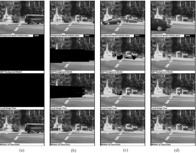
formu-lation is the ability to know when a well-defined initial back-ground model is ready to be used for tracking. We demonstrate this point by making comparisons with the popular mixture of Gaussians model [33] and the local image flow approach [16]. While the two methods are also effective for background ini-tialization, they both lack a clear definition of what an under-lying background scene is at any time instant of the estimation processes. For systems based on the mixture of Gaussians, they work by memorizing a certain number of modes for each pixel, and then by pixelwise integrating the most probable modes to form a background model. This is in essence a local scheme that the overall quality of a background model is difficult to evaluate. On the other hand, the method described in [16] is designed to process a whole image sequence to output a background model. We thus need to modify the algorithm into a sequential one so that the comparisons can be done by framewise examining the respectively derived background models.
The first experiment is carried out with image sequence where the three algorithms are alternately run till the image frame that our method completes its estimation for an initial background model. For the mixture model, we use three Gaussian distributions and a blending rate of 0.01, and initialize the background model at to the first image frame. For the local image flow implementation, the values of and are set to 30 and 15, and the background model is an empty set at . In Fig. 8, we show some intermediate results of ours and the corresponding background models produced by the other two methods. Due to the batch nature of the local image flow scheme, its three background models shown in Fig. 8 are obtained by running the algorithm three times, using the respec-tive periods of image frames as the inputs. Overall, the results produced by ours and the mixture of Gaussians are more re-liable than those of the local image flow, largely because the local flow scheme relies heavily on the estimations of optical flow directions and their accuracy. While the outcomes by the mixture of Gaussians seem to be satisfactory and similar to ours, the absence of a good measurement to guarantee the quality of the resulting background models remains a disadvantage of the approach. Furthermore, as one would expect that a mixture of
Gaussians method should be sensitive to lighting variations in that it is done by locally combining pixel intensities. We shall further elaborate on this issue with the next experiment.
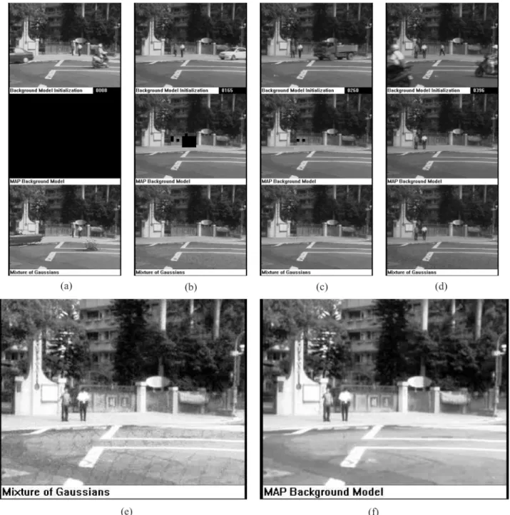
Our second comparison focuses on the effects of lighting changes. For the outdoor sequence (see Fig. 9), the lighting condition varies rapidly due to overcast clouds. And the exper-imental results show that our method is less sensitive to varia-tions of this kind. Specifically, in Fig. 9(e) and (f), we enlarge the sizes and enhance the contrasts of the two derived back-ground models for a clearer view. Note that especially in the road area our background model estimation is clearly of better quality than the one yielded by the mixture of Gaussians. This is mostly because of our uses of motion cues for identifying back-ground blocks and the properties of the MAP backback-ground model for integrating local and global consistency. On the other hand, the mixture of Gaussians approach uses only the pixelwise in-tensity information so that its performance depends critically on the variations of intensity distribution about the background scene.
5) Initialization and Tracking: To further illustrate the
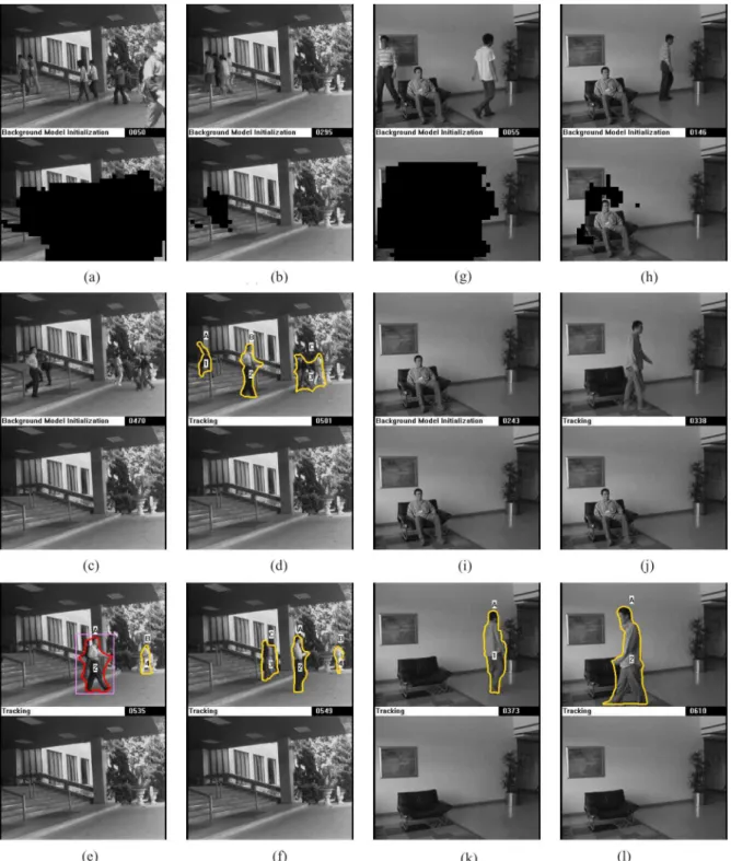
efficiency of using our proposed algorithm to estimate a back-ground model for tracking, we show the estimations of initial background models of test sequences and , and some subsequent tracking results in Fig. 10. Below each depicted image frame , the corresponding background model is plotted. In the two experiments, the estimations of the ini-tial background model are completed at frame number 470 and 243, respectively. Once the is available, the system can start to track objects immediately, using the scheme described in [4] (see Fig. 10). We also note that, as demonstrated in Fig. 10(j)–(l), the background model can be updated appropriately during tracking, even when significant changes in the scene background have occurred.
C. Discussions
An efficient online algorithm to establish a background model for tracking is proposed. The key idea of our approach is simple but effective: If one can tell whether an image block is part of the background, the additional knowledge can help to perform appropriate block updates. In addition, we introduce a global consistency check to eliminate noises in the updates. The two mechanisms, together, lead to a reliable system.
In background classifier learning, a classifier formulation with probability outputs is adopted so that the classification boundary can be easily tuned. While both an SVM and a CG-Boost classifier are appropriate for this purpose, the latter has an advantage of efficiency and is thus applied to the experiments. We also note that the relevance vector machines (RVMs) [34] are another possible choice. Particularly, RVMs are derived from MAP equations, and are truly probabilistic.
Regarding feature selection, two general motion cues, the in-terframe difference and the optical flow value, are adopted to discriminate background scenes. While the interframe differ-ence is effective in detecting static background blocks, the op-tical flow value, on the other hand, provides discriminability in classifying image blocks in small motions into gradually-varying background or moving foreground. To further justify
Fig. 8. Row one: Images frames from image sequenceA. Row two: Intermediate results of background estimation by our method that completes at t = 650. Row three and four: The results respectively derived by the local image flow approach [16] and the mixture of Gaussians method [33] at each corresponding time instant.
the use of the optical flow cue, additional evaluations using the interframe difference alone are provided. With the best setting of the difference threshold at 0.013, the training error is raised from 0.0466 to 0.0528 (or a 13.3% increase), and the testing error for the 20 evaluation image frames increases from 0.0378 to 0.0436 (or a 15.3% increase). Hence, the benefit of incorpo-rating the optical flow value is obvious.
About the three parameters, and , used in our method, only needs to be determined manually. Indeed, the exper-imental results demonstrate that the algorithm is robust to different parameter settings, and can handle lighting variations. Overall, our system is shown to be useful and practical for real-time tracking applications. For the future work, we are now extending the system to accommodate a pan/tilt/zoom camera. Such a modification would lead to a more challenging problem of simultaneous estimations of several initial background models.
APPENDIX
Described below are the derivations of the MAP formula-tion (2) in Secformula-tion II-A. For easy explanaformula-tion, the derivaformula-tions are decomposed into six parts, which are classifier training, it-erative formulation, posterior probability decomposition, like-lihood probability decomposition, background block classifica-tion, and the final MAP formulation.
1) Classifier Training: To begin with, a MAP
clas-sifier derived from the training data is defined by . It can be interpreted as a supervised learning process to train an optimal classifier from the training data . With the definition of , we can start to derive the following equations to estimate a background model:
where is assumed to peak at the optimal classifier (e.g., see [32, pp. 474–476]).
2) Iterative Formulation: To develop an iterative form for
estimating a background model, we first define
Fig. 9. Test sequenceB for lighting variations. (a)–(d) Due to overcast clouds, the outdoor lightings over the road change significantly throughout the sequence. As a result, the quality of background models yielded by the mixture of Gaussians is considerably affected. However, our formulation is more robust to such lighting perturbations. (e)–(f) Two derived background models att = 475 are enlarged and enhanced in contrast. False textures and extra noises can be observed in the road areas of (e). (a)B008, (b) B165, (c) B260, (d) B396, (e) Mixture of Gaussians, and (f) MAP.
Then we have
The image frames are used later to compute feature vectors for classification
where, similarly, is assumed to peak at
.
3) Posterior Probability Decomposition: Using Bayes’ rule,
we decompose into a product of an image
Fig. 10. Current image frameI and the derived background model ~B are plotted together, top and bottom, respectively. Some tracking results are also shown in theI s: (a) C050, (b) C295, (g) D055, (h) D146 (c) C470(t = 470), (d) C501, (i) D243(t = 243), (j) D338 (e) C535, (f) C549, (k) D373, and (l) D610.
Because the classifier is used to perform blockwise (local) classifications, and are those image frames used in computing feature values, both of them are eliminated from the
prior probability which is used to measure the global consis-tency over image blocks. That is, we simplify the prior term
from to .
4) Likelihood Probability Decomposition: Applying the
as-sumption of blockwise independencies, the likelihood term can be further decomposed as follows:
The term is reduced to , because is the th block of frame from an arbitrary online image stream, and it should be independent from our choice of a classifier and what the th block of a background model is at time , i.e., .
5) Background Block Classification: To utilize background
block classification in estimating a background model, we have
if is classified as background by otherwise
Then we derive the decomposition for the image likelihood
where is a background block and .
6) The Final MAP Formulation: With all these derivations,
we arrive at the following MAP optimization
ACKNOWLEDGMENT
The authors would like to thank the anonymous reviewers for their valuable comments on the manuscript of this paper.
REFERENCES
[1] P. M. Q. Aguiar and J. M. F. Moura, “Figure-ground segmentation from occlusion,” IEEE Trans. Image Process., vol. 14, no. 8, pp. 1109–1124, Aug. 2005.
[2] P. M. Q. Aguiar and J. M. F. Moura, “Joint segmentation of moving object and estimation of background in low-light video using relax-ation,” in Proc. 2007 IEEE Int. Conf. Image Processing, 2007, vol. 5, pp. 53–56.
[3] Y. Boykov, O. Veksler, and R. Zabih, “Fast approximate energy mini-mization via graph cuts,” IEEE Trans. Pattern Anal. Mach. Intell., vol. 23, no. 11, pp. 1222–1239, Nov. 2001.
[4] H.-T. Chen, H.-H. Lin, and T.-L. Liu, “Multi-object tracking using dynamical graph matching,” in Proc. Conf. Computer Vision Pattern
Recognition, Kauai, HI, 2001, vol. 2, pp. 210–217.
[5] S. Cohen, “Background estimation as a labeling problem,” in Proc. 10th
IEEE Int. Conf. Computer Vision, 2005, vol. 2, pp. 1034–1041.
[6] R. Cucchiara, C. Grana, M. Piccardi, and A. Prati, “Detecting moving objects, ghosts, and shadows in video streams,” IEEE Trans. Pattern
Anal. Mach. Intell., vol. 25, no. 10, pp. 1337–1342, Oct. 2003.
[7] F. De la Torre and M. Black, “Robust principal component analysis for computer vision,” in Proc. 8th IEEE Int. Conf. Computer Vision, Vancouver, Canada, 2001, vol. 1, pp. 362–369.
[8] A. Demiriz, K. Bennett, and J. Shawe-Taylor, “Linear programming boosting via column generation,” Mach. Learn., vol. 46, no. 1–3, pp. 225–254, 2002.
[9] A. Elgammal, D. Harwood, and L. Davis, “Nonparametric background model for background subtraction,” in Proc. 6h Eur. Conf. Computer
Vision, Trinity College, Dublin, Ireland, 2000, vol. 2, pp. 751–767.
[10] T. Ellis and M. Xu, “Object detection and tracking in an open and dy-namic world,” presented at the IEEE Int. Workshop Performance Eval-uation of Tracking and Surveillance, Kauai, HI, Dec. 9, 2001. [11] Y. Freund and R. Schapire, “Experiments with a new boosting
algo-rithm,” in Proc. 13th Int. Conf. Machine Learning, San Francisco, CA, 1996, pp. 148–156.
[12] B. J. Frey, N. Jojic, and A. Kannan, “Learning appearance and trans-parency manifolds of occluded objects in layers,” in Proc. Conf.
Com-puter Vision Pattern Recognition, 2003, vol. 1, pp. 45–52.
[13] J. Friedman, T. Hastie, and R. Tibshirani, “Additive logistic regression: A statistical view of boosting,” Ann. Statist., vol. 38, no. 2, pp. 337–374, Apr. 2000.
[14] N. Friedman and S. Russell, “Image segmentation in video sequences: A probabilistic approach,” in Proc. 13th Conf. Uncertainty in Artificial
Intelligence, San Francisco, CA, 1997, pp. 175–181.
[15] X. Gao, T. Boult, F. Coetzee, and V. Ramesh, “Error analysis of back-ground adaption,” in Proc. Conf. Computer Vision Pattern Recognition, Hilton Head Island, SC, 2000, vol. 1, pp. 503–510.
[16] D. Gutchess, M. Trajkovics, E. Cohen-Solal, D. Lyons, and A. Jain, “A background model initialization algorithm for video surveillance,” in
Proc. 8th IEEE Int. Conf. Computer Vision, Vancouver, Canada, 2001,
vol. 1, pp. 733–740.
[17] I. Haritaoglu, D. Harwood, and L. Davis, “A fast background scene modeling and maintenance for outdoor surveillance,” in Proc. 15th
Int. Conf. Pattern Recognition, Barcelona, Spain, 2000, vol. 4, pp.
179–183.
[18] E. Hayman and J.-O. Eklundh, “Statistical background subtraction for a mobile observer,” in Proc. 9th IEEE Int. Conf. Computer Vision, Nice, France, 2003, pp. 67–74.
[19] M. Heikkilä and M. Pietikäinen, “A texture-based method for modeling the background and detecting moving objects,” IEEE Trans. Pattern
Anal. Mach. Intell., vol. 28, no. 4, pp. 657–662, 2006.
[20] M. Irani and S. Peleg, “Motion analysis for image enhancement: Res-olution, occlusion, and transparency,” J. Vis. Commun. Image
Repre-sent., vol. 4, pp. 324–335, 1993.
[21] N. Jojic and B. J. Frey, “Learning flexible sprites in video layers,” in
Proc. Conf. Computer Vision Pattern Recognition, Kauai, HI, 2001,
vol. 1, pp. 199–206.
[22] D.-W. Kim and K.-S. Hong, “Practical background estimation for mosaic blending with patch-based Markov random fields,” Pattern
Recognit., vol. 41, no. 7, pp. 2145–2155, 2008.
[23] D.-S. Lee, “Effective Gaussian mixture learning for video background subtraction,” IEEE Trans. Pattern Anal. Mach. Intell., vol. 27, no. 5, pp. 827–832, 2005.
[24] B. Lucas and T. Kanade, “An iterative image registration technique with an application to stereo vision,” in Proc. DARPA IU Workshop, 1981, pp. 121–130.
[25] S. McKenna, S. Jabri, Z. Duric, A. Rosenfeld, and H. Wechsler, “Tracking groups of people,” Comput. Vision Image Understand., vol. 80, no. 1, pp. 42–56, Oct. 2000.
[26] A. Mittal and D. Huttenlocher, “Site modeling for wide area surveil-lance and image synthesis,” in Proc. Conf. Computer Vision Pattern
Recognition, Hilton Head Island, SC, 2000, vol. 2, pp. 160–167.
[27] A. Monnet, A. Mittal, N. Paragios, and V. Ramesh, “Background mod-eling and subtraction of dynamic scenes,” in Proc. 9th IEEE Int. Conf.
Computer Vision, Nice, France, 2003, pp. 1305–1312.
[28] J. Platt, “Probabilistic outputs for support vector machines and compar-isons to regularized likelihood methods,” in Advances in Large Margin
Classifiers, A. Smola, P. Bartlett, B. Scholkopf, and D. Schuurmans,
Eds. Cambridge, MA: MIT Press, 2000.
[29] G. Rätsch, T. Onoda, and K.-R. Müller, “Soft margins for adaboost,”
Mach. Learn., vol. 42, pp. 287–320, 2001.
[30] C. Ridder, O. Munkelt, and H. Kirchner, “Adaptive background esti-mation and foreground detection using kalman-filtering,” in Proc. Int.
[31] J. Rittscher, J. Kato, S. Joga, and A. Blake, “A probabilistic background model for tracking,” in Proc. 6th Eur. Conf. Computer Vision, Trinity College, Dublin, Ireland, 2000, vol. 2, pp. 336–350.
[32] B. Schölkopf and A. Smola, Learning With Kernels: Support Vector
Machines, Regularization, Optimization, and Beyond. Cambridge, MA: MIT Press, 2002, pp. 469–516.
[33] C. Stauffer and W. Grimson, “Adaptive background mixture models for real-time tracking,” in Proc. Conf. Computer Vision Pattern
Recog-nition, Fort Collins, CO, 1999, vol. 2, pp. 246–252.
[34] M. Tipping, “Sparse Bayesian learning and the relevance vector ma-chine,” J. Mach. Learn. Res., vol. 1, pp. 211–244, Jun. 2001. [35] K. Toyama, J. Krumm, B. Brumitt, and B. Meyers, “Wallflower:
Prin-ciples and practice of background maintenance,” in Proc. 7th IEEE Int.
Conf. Computer Vision, Corfu, Greece, 1999, vol. 1, pp. 255–261.
[36] D. Wang, T. Feng, H. Shum, and S. Ma, “A novel probability model for background maintenance and subtraction,” in Proc. 15th Int. Conf.
Vision Interface, Calgary, Canada, 2002, pp. 109–116.
[37] J. Wills, S. Agarwal, and S. Belongie, “What went where,” in Proc.
Conf. Computer Vision Pattern Recognition, 2003, vol. 1, pp. 37–44.
[38] C. Wren, A. Azarbayejani, T. Darrell, and A. Pentland, “Pfinder: Re-altime tracking of the human body,” IEEE Trans. Pattern Anal. Mach.
Intell., vol. 19, no. 7, pp. 780–785, Jul. 1997.
Horng-Horng Lin (S’07) received the B.S. degree in computer science and information engineering and the M.S. degree in computer and information science both from National Chiao Tung University, Taiwan, in 1997 and 1999, respectively. He is currently working towards the Ph.D. degree at the Department of Computer Science at National Chiao Tung University, Taiwan.
Between 1999 and 2004, he served the National Defense Substitute Service on Enterprise, as a Re-search Assistant at the Institute of Information Sci-ence in Academia Sinica, Taiwan. His research interests include computer vi-sion and machine learning.
Tyng-Luh Liu (M’99) received the B.S. degree in ap-plied mathematics from the National Chengchi Uni-versity, Taiwan, in 1986 and the Ph.D. degree in com-puter science from New York University in 1997.
He is an Associate Research Fellow of the Institute of Information Science at Academia Sinica, Taiwan. His research has focused on computer vision and pat-tern recognition.
Dr. Liu received the Research Award for Junior Re-search Investigators from Academia Sinica in 2006.
Jen-Hui Chuang (S’86–M’91–SM’06) received the B.S. degree in electrical engineering from National Taiwan University in 1980, the M.S. degree in elec-trical and computer engineering from the University of California at Santa Barbara in 1983, and the Ph.D. degree in electrical and computer engineering from the University of Illinois at Urbana-Champaign in 1991.
Since 1991, he has been on the faculty of the Department of Computer Science at National Chiao Tung University, Hsinchu, Taiwan, where he is currently a Professor. His research interests include robotics, computer vision, 3-D modeling, and image processing.