An efficient algorithm for finding the D-stability bound of discrete singularly perturbed systems with multiple time delays

Publisher: Taylor & Francis

Informa Ltd Registered in England and Wales Registered Number: 1072954 Registered office: Mortimer House, 37-41 Mortimer Street, London W1T 3JH, UK

International Journal of Control

Publication details, including instructions for authors and subscription information:

http://www.tandfonline.com/loi/tcon20

An efficient algorithm for finding the

D-stability bound of discrete singularly perturbed

systems with multiple time delays

Feng-Hsiag Hsiao

Published online: 08 Nov 2010.

To cite this article: Feng-Hsiag Hsiao (1999) An efficient algorithm for finding the D-stability bound of discrete singularly perturbed systems with multiple time delays, International Journal of Control, 72:1, 1-17, DOI: 10.1080/002071799221352

To link to this article: http://dx.doi.org/10.1080/002071799221352

PLEASE SCROLL DOWN FOR ARTICLE

Taylor & Francis makes every effort to ensure the accuracy of all the information (the “Content”) contained in the publications on our platform. However, Taylor & Francis, our agents, and our licensors make no representations or warranties whatsoever as to the accuracy, completeness, or suitability for any purpose of the Content. Any opinions and views expressed in this publication are the opinions and views of the authors, and are not the views of or endorsed by Taylor & Francis. The accuracy of the Content should not be relied upon and should be independently verified with primary sources of information. Taylor and Francis shall not be liable for any losses, actions, claims, proceedings, demands, costs, expenses, damages, and other liabilities whatsoever or howsoever caused arising directly or indirectly in connection with, in relation to or arising out of the use of the Content.

This article may be used for research, teaching, and private study purposes. Any substantial or systematic reproduction, redistribution, reselling, loan, sub-licensing, systematic supply, or distribution in any form to anyone is expressly forbidden. Terms & Conditions of access and use can be found at http://www.tandfonline.com/page/terms-and-conditions

An e cient algorithm for ® nding the D-stability bound of discrete singularly perturbed systems with

multiple time delays

FENG-HSIAG HSIAO² , SHING-TAI PAN³ and CHING-CHENG TENG§

In this paper, we present an original work on the D-stabilization problem of discrete singularly perturbed systems with multiple time delays. A new robust D-stability criterion in terms of stability radius is ® rst derived to guarantee that all poles of the discrete multiple time-delay systems remain inside the speci® c disk Da

,

r in the presence of parametric

uncertainties. Then, by using the technique of time-scale separation, we derive the corresponding slow and fast sub-systems of a discrete multiple time-delay singularly perturbed system. The state feedback controls for the D-stabilization of the slow and the fast subsystems are separately designed and a composite state feedback control for the original system is subsequently synthesized from these state feedback controls. Thereafter, we derive a frequency domaine -dependent

D-stability criterion for the original discrete multiple time-delay singularly perturbed system under the composite state feedback control. If any one of the conditions of this criterion is ful® lled, D-stability of the original closed-loop system is thus investigated by establishing that of its corresponding slow and fast closed-loop subsystems. Finally, an e cient algorithm is proposed to obtain a less conservative D-stability bound of the singular perturbation parameter and to reduce the computation time.

1. Introduction

In the analysis of dynamic systems, we are often faced with parametric uncertainties originating from various sources, e.g. identi® cation errors, ageing of devices, variation of operating points, etc. Therefore, the problem of maintaining the stability of a nominally stable system subject to uncertainties has been of con-siderable interest to researchers and a number of signif-icant results concerning this issue have been reported in the literature. On the other hand, the problem of pole assignment in linear systems theory has been discussed by many authors and solved in various ways. However, one cannot place the poles at a speci® c location, due to parametric uncertainties. Therefore, placing all poles in a speci® c region rather than choosing an exact assign-ment may be satisfactory in practical applications. One

such speci® c region for discrete systems is a disk D

a

,

r

centred at

a

,

0 with radius r, where

a

r < 1. The

assignment of all poles of a system in the speci® c disk

D

a

,

r shown in ® gure 1 is referred to as a D-pole

pla-cement problem (Furuta and Kim 1987

)

. This subject

has received much attention in previous reports (Furuta and Kim 1987, Lee and Lee 1987, Kolla et al. 1989,

Vicino 1989, Lee et al. 1992, Su and Shyr 1994

)

.

The stability radius is a tool to describe the distance from instability. There are two distances from instability for a real square matrixÐ the complex stability radius and the real stability radius; they can di€ er considerably. In general, the real stability radius is more important in applications but is more di cult to determine

(Hinrichsen and Pritchard 1986

)

. Kharitonov (1991

)

has been concerned with the analysis of the complex stability radius of a matrix with respect to the unit disk of the complex plane.

The problem of stabilizing time-delay systems has been explored over the years because delay is commonly encountered in various engineering systems, such as chemical processesÐ e.g. steel smelting and re® ningÐ or in long transmission lines, in pneumatic, hydraulic or electric networks. Its existence may produce undesir-able system responses. Consequently, researchers on sta-bility analysis of time-delay systems become essential to practical applications. This question has been raised by

Mori et al. (1982

)

, Mori (1985

)

, Mori and Kokame

(1989

)

, Oucheriah (1995

)

, Wang and Wang (1995

)

,

Hsiao and Hwang (1996a), and others. Since the number of poles of the closed-loop system increases due to time delays, the introduction of a time-delay factor makes the D-pole placement problem much more complicated. The D-stability problem for discrete time-delay systems has

been discussed by Lee et al. (1992

)

and Su and Shyr

(1994

)

. However, their results are too conservative.

Furthermore, there exist multiple time delays in some physical systems and delays in practice are not exact integer multiples of the sampling interval. Thus, for the purpose of general application, two cases of a new robust D-stability criterion in terms of complex stability radius are proposed for discrete uncertain systems with multiple time delays which may not be exact integer

0020-7179/99 $12.00Ñ 1999 Taylor & Francis Ltd. Received 19 August 1997. Revised 30 March 1998.

² _{Department of Electrical Engineering, Chang Gung} Uni-versity, 259 Wen-Hwa 1st Road, Kwei-San, Taoyuan Shian, Taiwan 333, R.O.C. (Author for correspondence).

³ Department of Electrical Engineering, Kao Yuan

Insti-tute of Technology, 1821 Chung-Shan Road, Lu-Chu, Kaoh-siung Shian, Taiwan 821, R.O.C.

§Institute & Department of Control Engineering, National Chiao Tung University, 1001 Ta Hsueh Road, Hsinchu, Tai-wan 300, R.O.C.

multiples of the sampling interval. One is a direct test

(i.e., check d1< ds

)

and the other is a boundary test. The

robust D-stability is ® rst checked by the direct test. If it fails, resort to the boundary test.

Singularly perturbed systems have been studied by many researchers (see, for example, Saksena et al. 1984, Kokotovic et al. 1986, Su and Hsieh 1990, Chen and Hsieh 1994, Chen et al. 1994, Venkatasubramanian

1994, Hsiao and Hwang 1996b

)

. This is due not only

to theoretical interest but also to the relevance of this topic to the control of engineering applications. The singular perturbation parameters often result from the presence of small parameters in various physical systems; e.g. in power system models the singular per-turbation parameters can represent machine reactances or transients in voltage regulators. In industrial control systems they may represent time constants of drives and actuators, and in nuclear reactor models they are due to fast neutrons, etc. (Kokotovic et al. 1976). Indeed, the singular perturbation approach has been proven to be a powerful tool for system analysis and control design (Corless and Glielmo 1991). A fundamental feature of such an approach is that the feedback design problem can be broken into two design subproblems for the slow and fast subsystems. The two designs are then combined

to give a design for the original systems (Khalil 1989

)

.

A key to the analysis of singularly perturbed systems thus lies in the construction of the slow and fast subsys-tems. It is noted that the approximation of an original, singularly perturbed system via its corresponding slow and fast subsystems is valid only when the singular per-turbation parameters of this system are su ciently small. Therefore, it is important to ® nd the stability bound of singular perturbation parameters such that the stability of the original system can be investigated by establishing that of its corresponding slow and fast subsystems, provided that the singular perturbation par-ameters are su ciently small to be within this bound. For a continuous-time system, Klimushchev and

Krasovskii (1962)found thee -bound of singularly

per-turbed systems. In Feng (1988), Chen and Lin (1990)

and Lin and Chen (1992), a frequency-domain approach

was proposed to ® nd the e -bound of singularly

per-turbed systems. Shao and Rowland (1995) considered

a linear time-invariant singularly perturbed system with single time delay in the slow states. Their work gave a delay-independent su cient condition for the

stability bound of e . In cases of discrete time, the

two-time-scale properties of weakly coupled discrete systems and control of these systems were discussed by Mahmoud (1982). The stability bound of singular per-turbation parameters for the asymptotic stability analy-sis of singularly perturbed systems with a single

parameter was discussed by Li and Li (1992

)

.

In this paper, the research on time-scale modelling is extended to include discrete multiple time-delay singu-larly perturbed systems. The stability problem of dis-crete multiple time-delay singularly perturbed systems was ® rst considered by Trinh and Aldeen (1995), in whose paper time delays are exact integer multiples of the sampling interval. In their work, the delay terms are treated as the perturbations of the systems and the

sta-bility bound of e is obtained from nominal systems. As

for the singular perturbation approach, they merely dealt with discrete singularly perturbed systems without delay and subject to some plant uncertainties. In our work, the control design for discrete singularly per-turbed systems with multiple time delays which may not be exact integer multiples of the sampling interval is ful® lled by using the standard procedure to analyse singularly perturbed systems. Furthermore, an e cient algorithm for ® nding the D-stability bound of the sin-gular perturbation parameter is proposed.

The organization of this study is as follows. In §2,

the techniques of D-pole placement and complex stabi-lity radius are combined and extended such that they

can solve the D

a

,

r -stability problem of discrete

uncer-tain multiple time-delay systems. Two cases of a new robust D-stability criterion in terms of complex stability radius are proposed to guarantee that all poles of the

system remain inside the speci® ed disk D

a

,

r in the

presence of parametric uncertainties. The corresponding slow and fast subsystems of a discrete multiple time-delay singularly perturbed system are then derived in §3. In §4, the state feedback controls for the slow and fast subsystems are separately designed such that the

slow and fast closed-loop subsystems are both D

a

,

r

-stable. In§5, a composite state feedback control for the

original system is synthesized from the state feedback

controls designed in §4 and a frequency domain e

-dependent D-stability criterion is subsequently proposed to examine whether the singular perturbation parameter

e is small enough or not. Ife is so small that any one of

the conditions of this criterion is satis® ed, then D

a

,

r

-stability of the slow and fast closed-loop subsystems can imply the stability of the original system under the com-Figure 1. A disk Da

,

r centred at a

,

0 with radius r.

posite state feedback control. In order to obtain a less conservative D-stability bound of the singular perturba-tion parameter and to reduce the computaperturba-tion time, an

e cient algorithm is proposed in §6. Finally, an

ex-ample is provided to illustrate the e cient algorithm.

2. D-stability criterion

In this section, we will propose a new robust D-sta-bility criterion in terms of complex staD-sta-bility radius for discrete uncertain multiple time-delay systems described by the following di€ erence equation:

x k 1 Ax k D Ax k n i 1 Adix k hi n i 1 D Adix k hi 2.1

in which A and Adi are constant matrices with

appro-priate dimensions and hi, i 1

,

2

,

. . .

,

n, are positive

numbers: D A and D Adi denote the parametric

uncer-tainties with the following upper norm-bounds:

D A b 2.2 a

D Adi

h

i

,

i 1

,

2

,

. . .

,

n

,

2.2 b

whereb and

h

iare given constants.

Before we proceed to derive the robust D-stability criterion, some useful concepts are given in the follow-ing.

De® nition 1: A feedback control system is said to be

D

a

,

r -stable if all poles of the system are within the

speci® c disk D

a

,

r centred at

a

,

0 with radius r. In

other words, the solutions of its characteristic equation satisfy

z

a

/r < 1 2.3

in which r > 0 and

a

r < 1.

De® nition 2(Hinrichsen and Pritchard 1988,

Kharito-nov 1991): Let all eigenvalues of the matrix A be

in-side the unit circle of the complex plane; then the positive value

q A max

0 µ 2p e

jµ_{I A} 1 1 ₂

.4 is said to be a complex stability radius of the matrix A. Remark 1 (Kharitonov 1991): The value q A

de-pends on the choice of norm. For instance, if the Eu-clidean norm is used, then it is easy to show that

µA min

0 µ 2p s e

jµ_{I A}

,

₂

.5

in whichs is the minimal singular value of matrix .

Lemma 1 (Kharitonov 1991): Let all eigenvalues of

the matrix M be inside the unit disk of the complex

plane. All the eigenvalues of all matrices M D M are

inside the unit disk if and only if D M <q M .

Lemma 2 (Vidyasagar 1985): Let a matrix

E z Rm n, with Rm n denoting the set of m n

ma-trices whose elements are proper stable rational func-tions; then sup z X E z supz 1 E z µsup0,2p E ejµ 2.6 where X z r

,

ejµ

,

µ 0

,

2

p

,

r 1 . Since E z is

analytic for z X , this norm is well de® ned.

After reviewing the above de® nitions and lemmas, we are in the position to derive the robust D-stability criterion in terms of complex stability radius for a dis-crete uncertain multiple time-delay system.

Theorem 1:

(I) Suppose that all the eigenvalues of A are within

the speci® c disk D

a

,

r . The system 2.1 is

robustly D

a

,

r -stable if 1 r b n i 1 Adi

h

i r

a

hi d1<q A

a

I r ds

,

2.7a in which

a

< r.

(II

)

If d1 ds and the function

h g 1 r b n i 1 Adi rg

a

hi n i 1

h

i r

a

hi _2.7b

does not lie inside the interval ds

,

d1, where

a

< r and g takes the values in the bounded

region U1 g g r ejµ

,

µ 0

,

2

p

,

1 r d_1r

with

d1r A _r

a

I d1

then the system (2.1

)

is robustly D

a

,

r -stable.

Proof: See Appendix A.

Remark 2: It is easy to see that the D-stability cri-terion in Theorem 1 will get a less conservative result

than the criteria proposed by Lee et al. (1992) and Su

and Shyr (1994). Furthermore, since system (2.1)

con-tains multiple time delays which may not be exact

ger multiples of the sampling interval, their results can-not examine the D-stability of system (2.1).

Remark 3: Case (I) of Theorem 1 provides a neat al-gebraic condition to test the D-stability of system (2.1) at the cost of conservativeness. It is therefore

reason-able to check the D-stability with case (I) and then, if

it fails, to resort to case (II). Thus, case (I) and case

(II)complement each other.

However, for a practical application, it is di cult to

examine case (II)of Theorem 1. The following

`bound-ary test’ may be helpful in examining this case.

Corollary 1: If d1 ds and the following inequality

(2.8

)

holds: h g 1 r b n i 1 Adi rg a hi n i 1h i r a hi < ds 2.8 where

a

< r and g ejµ

forµ 0

,

2

p

, then the system

(2.1)is robustly D

a

,

r -stable.

Proof: The matrix ni 1Adi rg

a

hi of which all

poles of the elements have the modulus

g

a

_{r <}1 2.9

belongs toRm m. Consequently, on the basis of Lemma

2, the term ni 1Adi rg

a

hi in (2.8) takes on its

supremum in the range given by g ejµ_for

µ 0

,

2

p

.

Therefore, if the inequality (2.8

)

holds, h g does not lie

inside the interval [ds

,

d1] for all g U1 and then the

system (2.1)is robustly D

a

,

r -stable (according to the

case (II

)

of Theorem 1). This completes the proof. h

3. Problem formulation

Consider the following discrete multiple time-delay singularly perturbed system:

x1 k 1 n i 0 A1ix1 k hi e n i 0 ~ A1ix2 k hi B1u k 3.1 a x2 k 1 n i 0 A2ix1 k hi e n i 0 ~ A2ix2 k hi B2u k 3.1 b

where A1i, A2i,A~1i,A~2i, i 0

,

1

,

2

,

. . .

,

n, B1and B2are

constant matrices with appropriate dimensions and hi,

i 1

,

2

,

. . .

,

n, are positive numbers h0 0 ; the pair

A10

,

B1 is assumed to be controllable. System (3.1)is

referred to as the C-model (p. 45, Naidu and Rao 1985)

and can be obtained from the slow sampling rate model as a result of discretization or sampled-data control of singularly perturbed continuous-time systems (Li and Li

1992). The small positive scalare is a singular

perturba-tion parameter subject to the following constraint:

e

n i 0

~

A2i < 1. 3.2

Before we discuss the main result, a lemma is ® rst given in the following.

Lemma 3 (Chou and Chen 1990): For any matrix

A Rm m_{, if s A < 1² , then det I A > 0.}

On the basis of Lemma 3 and the fact that s e n i 0 ~ A2i e n i 0 ~ A2i e n i 0 ~ A2i < 1

it is clear that the matrix

I e

n i 0

~

A2i

is non-singular. Now, according to the time-scale analy-sis in Mahmoud (1982), the slow and fast subsystems of

the original system (3.1)can then be derived as follows.

3.1. The slow subsystem

Let x2 k hi x2 k x2 k for i 1

,

2

,

. . .

,

n; the

system (3.1)thus reduces to

xs k 1 n i 0 A1ixs k hi e n i 0 ~ A1i x2 k B1us k 3.3a x2 k n i 0 A2ixs k hi e n i 0 ~ A2i x2 k B2us k 3.3b

where xs, x2and us are the slow components of x1, x2

and u, respectively. From equation (3.3 b), we have

² The notation s A denotes the spectral radius of the

matrix A.

x2 k I e n i 0 ~ A2i 1 n i 0 A2ixs k hi I e n i 0 ~ A2i 1 B2us k 3.4

Substituting (3.4)into (3.3a), the slow subsystem of the

original system (3.1)can be expressed as

xs K 1 n i 0 Asixs k hi Bsus k 3.5 a where Asi A1i e n j 0 ~ A1j I e n j 0 ~ A2j 1 A2i for i 0

,

1

,

2

,

. . .

,

n 3.5 b Bs B1 e n i 0 ~ A1i I e n i 0 ~ A2i 1 B2. 3.5 c

3.2. The fast subsystem Let

xf k x2 k x2 k

,

uf k u k us k

,

usk us k hi

and

x1 k x1 k hi xs k hi xs k

for i 1

,

2

,

. . .

,

n; we have (from equation (3.4

))

xf k x2 k I e n i 0 ~ A2i 1 _n i 0 A2i xs k I e n i 0 ~ A2i 1 B2us k 3.6

According to equation (3.1 b), the fast subsystem of the

original system (3.1)is derived as follows:

xf k 1 e n i 0 ~ A2ixf k hi e n i 0 ~ A2i I e n i 0 ~ A2i 1 _n i 0 A2i xs k e n i 0 ~ A2i I e n i 0 ~ A2i 1 B2us k n i 0 A2i xs k B2uf k us k I e n i 0 ~ A2i 1 _n i 0A2i xs k I e n i 0 ~ A2i 1 B2us k e n i 0 ~ A2ixf k hi n i 0A 2i I e n i 0 ~ A2i I e n i 0 ~ A2i 1 _n i 0A2i xs k B2uf k I I e n i 0 ~ A2i I e n i 0 ~ A2i 1 B2us k n i 0Afixf k hi Bfuf k 3 .7 a where Afi e A2i and Bf B2. 3.7b

4. State feedback controls for the slow and fast subsystems

In this section, the state feedback controls for the

slow subsystem (3.5) and for the fast subsystem (3.7)

are separately designed such that both slow and fast

closed-loop subsystems are D

a

,

r -stable.

4.1. State feedback control for the slow subsystem Introducing the slow control

us k n i 0

ksixs k hi 4.1

in which ksi, i 0

,

1

,

2

,

. . .

,

n, are the state feedback

gains into the slow subsystem (3.5), we have

xs k 1 n i 0 Asi Bsksi xs k hi n i 0 A1i D A1i e B1 D B1 e ksi xs k hi n i 0 Asi D Asi e xs k hi 4.2

in which Asi A1i B1ksi

,

D Asi e D A1i e D B1 e ksi 4.3 with D A1i e e n i 0 ~ A1j I e n i 0 ~ A2j 1 A2i

,

i 0

,

1

,

2

,

. . .

,

n D B1e e n i 0 ~ A1j I e n i 0 ~ A2j 1 B2.

On the basis of the constraint (3.2

)

, we can derive the

following inequality: I e n i 0 ~ A2i 1 I e n i 0 ~ A2i e 2 n i 0 ~ A2i 2 I e n i 0 ~ A2i e 2 n i 0 ~ A2i 2 1 e n i 0 ~ A2i e 2 n i 0 ~ A2i 2 1 1 e n i 0 ~ A2i 4.4 a

According to the inequality (4.4 a

)

, we have

D A1i e e n j 0 ~ A1j I e n j 0 ~ A2j 1 A2i e n j 0 ~ A1j I e n j 0 ~ A2j 1 A2i e n k 0 ~ A1j A2i 1 e n j 0 ~ A2j

a

i e

,

i 0

,

1

,

2

,

. . .

,

n 4.4 b D B1e e n j 0 ~ A1j I e n j 0 ~ A2j 1 B2 e n j 0 ~ A1j I e n j 0 ~ A2j 1 B2 e n j 0 ~ A1j B2 1 e n j 0 ~ A2j b e

,

4.4 c and hence D Asi e D A1i e D B1e ksi D A1i e D B1e ksi

a

i e b e ksi d i e

,

i 0

,

1

,

2

,

. . .

,

n. 4.5

Consequently, according to case (I)of Theorem 1, if the

state feedback gains ksi

,

i 0

,

1

,

2

,

. . .

,

n, are chosen

such that d1s 1_r d 0e n i 1 Asi d i e r

a

hi <q As0_r

a

I dss

,

4.6a

then the slow closed-loop subsystem (4.2

)

, or

equiva-lently the slow subsystem (3.5

)

under the control (4.1

)

,

is D

a

,

r -stable with r >

a

. Substituting (4.5) into

(4.6 a)and according to (4.4 b)and (4.4 c), the inequality

(4.6 a)is equivalent to e < ns ms ns n i 0 ~ A2i e 1 4.6b where ns rdss n i 1 Asi r

a

hi² and ms n i 0 ~ A1i n i 0 A2i B2 ksi r

a

hi .

² According to (4.6 a), it is obvious that nsis positive.

However, if the condition (4.6a), or equivalently (4.6b), fails, then we resort to checking the following condition (see Corollary 1): hs g 1_r d 0 e n i 1 Asi rg

a

hi n i 1 d i e r

a

hi < dss

,

4.7

where r >

a

and g ejµ_for

h

₀

,

₂

p

_.

Remark 4: For the purpose of D

a

,

r -stabilization of slow closed-loop subsystem (4.2), the state feedback

gains ksi, i 0

,

1

,

2

,

. . .

,

n, are adjusted such thate ₁ is

as large as possible. This can be ful® lled by choosing

ks0 to place all the poles of As0 A10 B1ks0 at

a

,

0

(i.e. to maximize dss

)

and choosing ksi to minimize

Asi A1i B1ksi for i 1

,

2

,

. . .

,

n. However,

there are various choices of ksi, i 0

,

1

,

2

,

. . .

,

n, to

make e 1 as large as possible, but only one of them is

chosen here.

Remark 5: The inequality (4.6 b)provides a neat

alge-braic equation to ® nd the upper bound of e , which

guarantees the D

a

,

r -stability of the slow closed-loop

subsystem (4.2) at the cost of conservativeness.

How-ever, a less conservative upper bound, called~e ₁, can be

obtained by ® nding the upper bound of e that ful® ls

the inequality (4.7)with much more computation time.

4.2. State feedback control for the fast subsystem Introducing the fast control

uf e

n i 0

kfixf k hi 4.8

where kfi, i 0

,

1

,

2

,

. . .

,

n, are the state feedback gains

into the fast subsystem (3.7), we have

xf k 1 n i 0 Afixf k hi e Bf n i 0 kfixf k hi n i 0 Afi e Bfkfi xf k hi n i 0 e A~2i Bfkfi xf k hi n i 0 D Afi e xf k hi 4.9 a in which D Afi e e A~2i Bfkfi 4.9 b

Consequently, according to case (I)of Theorem 1, if the

state feedback gains kfi, i 0

,

1

,

2

,

. . .

,

n, are chosen

such that d1f 1_r D Af 0 n i 0 D Afi r

a

hi 1 r n i 0 D Afi r

a

hi <q

a

_rI dsf 4.10a

then the fast closed-loop subsystem (4.9), or equivalently

the fast subsystem (3.7) under the control (4.8), is

D

a

,

r -stable with r >

a

. It is noted that the inequality

(4.10 a) is equivalent to e < _n rdsf i 0 ~ A2i Bfkfi r

a

hi e 2 4.10b

However, if the condition (4.10 a), or equivalently (4.10 b), fails, then we resort to checking the following condition:

hf g 1_r

n i 0

D Afi rg

a

hi < dsf 4.11

where r >

a

and h ejµ_for

µ 0

,

2

p

.

Remark 6: In order to makee ₂ as large as possible,

according to the similar discussion in the preceding

subsection, we need only to choose k_~ fi to minimize

A2i Bfkfi for i 0

,

1

,

2

,

. . .

,

n. Moreover, e ₂

ob-tained from the more conservative inequality (4.10b)

(i.e. (4.10 a)) is less than the upper bound of e , called

~

e ₂, that ful® ls the inequality (4.11).

5. D(a , r)-stabilization of the original system

In this section, a composite state feedback control for the D-stabilization of the original discrete multiple

time-delay singularly perturbed system (3.1

)

is

sub-sequently synthesized from the slow control (4.1

)

and

the fast control (4.8

)

. Furthermore, a frequency domain

e -dependent D-stability criterion is derived such that the

D

a

,

r -stability of the original system (3.1

)

under the composite state feedback control can be investigated by establishing that of its corresponding slow

closed-loop subsystems (4.2) and fast closed-loop subsystem

(4.9).

According to the slow control (4.1)and the assertion

xs k hi xs k in §3.2, equation (3.6) can be

written as xf k x2 k I e n i 0 ~ A2i 1 _n i 0 A2i xs k I e n i 0 ~ A2i 1 B2 n i 0 ksixs k hi x2 k I e n i 0 ~ A2i 1 _n i 0 A2i xs k I e n i 0 ~ A2i 1 B2 n i 0 ksixs k 5.1 i.e. x2k xf k I e n i 0 ~ A2i 1 n i 0 A2i B2 n i 0 ksi xs k 5.2 Hence, we have x2 k hi xf k hi I e n i 0 ~ A2i 1 n i 0 A2i B2 n i 0 ksi xs k hi f or i 0

,

1

,

2

,

. . .

,

n 5.3

Consequently, the composite state feedback control is of the following form:

u k us k uf k n i 0 ksixs k hi n i 0 e kfixf k hi n i 0 ksi e kfi I e n j 0 ~ A2j 1 n j 0 A2j B2 n j 0 ksj xs k hi n i 0 e kfi I e n j 0 ~ A2j 1 n j 0 A2j B2 n j 0 ksj xs k hi xf k hi 5.4

On the basis of equation (5.3) and the assertion

xs k hi x1 k hi in §3.2 for i 0

,

1

,

2

,

. . .

,

n, the

composite feedback control (5.4)becomes

u k n i 0 k1ix1k hi n i 0 k2ix2k hi 5.5a where k1i ksi e kfi I e n i 0 ~ A2j 1 _n i 0 A2j B2 n i 0 ksj f or i 0

,

1

,

2

,

. . .

,

n 5.5b k2i e kfi f or i 0

,

1

,

2

,

. . .

,

n 5.5 c

Applying the composite state feedback control (5.5)to

the original system (3.1), we have x1 k 1 n i 0 M1ix1 k hi n i 0 M2ix2 k hi 5.6 a x2 k 1 n i 0 M3ix1 k hi n i 0 M4ix2 k hi 5.6 b where M1i A1i B1k1i

,

M2i e A~1i B1k2i M3i A2i B2k1i

,

M4i e A~2i B2k2i 5.6 c

Prior to discussing D

a

,

r -stabilization problem of

the closed-loop system (5.6

)

, we ® rst introduce a useful

lemma as follows.

Lemma 4 (maximum modulus theorem

)

(John

1967

)

: If f z is analytic in a bounded domain D and

continuous in D (i.e. the closure of D

), then f z takes

its maximum on the boundary of D.

We now proceed to derive a frequency domain e

-dependence D-stability criterion for the closed-loop system (5.6).

Theorem 2: If the state feedback gains ksi and kfi for

i 0

,

1

,

2

,

. . .

,

n are chosen such that the slow

closed-loop subsystem (4.2

)

and the fast closed-loop subsystem

(4.9

)

are both D

a

,

r -stable with r >

a

, the original

system (3.1

)

under the composite state feedback control

(5.5), or equivalently system (5.6), is D

a

,

r -stable with

r >

a

if the singular perturbation parametere satis® es

I q u~~_g e

,

ejµ < 1 forµ 0

,

2

p

5.7a

or

II q u~~~_g e

,

ejµ < 1 forµ 0

,

2

p

5.7b

where ~ u _g~ _e

,

ejµ L~~_g1 _e

,

ejµ R~_g~ _e

,

ejµ n i 0 M2i e r e jµ a hi r ejµ a _I n i 0 M4i e r e jµ a hi 1 n i 0 M3i e r e jµ a hi and ~~ u _g~ e

,

ejµ R~~_g e

,

ejµ n i 0 M2i e re jµ

a

hi r e jµ

a

_I n i 0 M4i e r e jµ

a

hi 1 n i 0 M3i e r e jµ

a

hi

L

~~_g1 e

,

ejµ with ~ L ~_ge

,

ejµ r e jµ a I n i 0 Asi e Bse ksi r e jµ a hi and ~ R~_g e

,

ejµ n i 0 e n i 0 ~ A1j I e n i 0 ~ A2j 1 A2i B2ksi e B1kfi I e n i 0 ~ A2j 1 n i 0 A2j B2ksj r e jµ

a

hi

Proof: See Appendix B.

Remark 7: The dependence of the matrices Mji for

j 2, 3, 4 and i 0

,

1

,

2

,

. . .

,

n upon e , although

omitted elsewhere, is indicated here in Theorem 2 for the purpose of clari® cation.

Remark 8: In principle, both the two conditions in

(5.7

)

can be used to test the D-stability of the

closed-loop system (5.6

)

. It is therefore reasonable to check

the D-stability with any one of the inequalities and then, if it fails, to resort to another.

Remark 9: Let e ₃ and ~e ₃ be the upper bounds of e

that ful® l the D-stability conditions (5.7 a) and (5.7b),

respectively. Since there is no explicit information to

indicate the conservativeness of e ₃and~e ₃, the less

con-servative one should be used to ® nd the D-stability

bound of e for each case in hand.

6. Algorithm for ® nding the D-stability bound "*

According to Theorem 2, the D-stability bound of e ,

callede , can be obtained by ® nding the uppere -bound

such that not only the slow closed-loop subsystem (4.2

)

and the fast closed-loop subsystem (4.9

)

are both

D

a

,

r -stable but also the condition (5.7a

)

or (5.7 b

)

is

satis® ed for alle 0

,

e . In order to obtain a less

con-servative result and to reduce the computation time, on the basis of Remarks 4± 6 and 9, we propose an e cient

algorithm to ® nd the D-stability bound e such that

D

a

,

r -stability of the slow closed-loop subsystem

(4.2) and the fast closed-loop subsystem (4.9) can

imply that of the original closed-loop system (5.6), provided that the singular perturbation parameter is su -ciently small to be within this bound.

Algorithm:

Step 1. Choose ks0 to place all the eigenvalues of

As0 A10 B1ks0 at

a

,

0 and choose ksi to

minimize Asi A1i B1ksi for i 1

,

2

,

. . .

,

n, and then we can obtaine 1from (4.6 b

)

.

Step 2. Choose kfi to minimize A~2i Bfkfi for

i 0

,

1

,

2

,

. . .

,

n, and then we can obtain e 2

from (4.10 b).

Step 3. Find the upper bound of e 3 such that the

inequality (5.7 a)holds for alle 0

,

e 3 .

Step 4. Choosee min e 1

,

e 2

,

e 3 .

Step 5. Ife e j, j 1

,

2 and 3, then go to (1), (2)and

(3), respectively.

(1) Find the upper bound ~_{e 1 such that (4.7)}

holds for all e 0

,

~e 1 and e

min ~e 1

,

e 2

,

e 3. If e ~e 1, then stop; else

go to Step 6.

(2

)

Find the upper bound~_{e 2 such that (4.11}

₎

holds for all e 0

,

~e 2 and e

min e 1

,

~e 2

,

e 3. If e ~e 2, then stop; else

go to Step 7.

(3) Find the upper bound~e 3such that (5.7b)

holds for all e 0

,

~e 3 . If ~e 3>e 3, then

e min e 1

,

e 2

,

~e 3 . Under this condition,

if e ~e 3, then stop; else go to Step 8.

However, if~_{e 3 e 3, then stop.}

Step 6. If e e j, j 2 and 3, then go to (1)and (2),

respectively.

(1) Find the upper bound~_{e 2 such that (4.11)}

holds for all e 0

,

~e 2 and e

min ~e 1

,

~e 2

,

e 3. If e ~e 2, then stop; else

go to Step 11.

(2) Find the upper bound~_{e 3 such that (5.7 b)}

holds for all e 0

,

~e 3. If ~e 3>e 3, then

e min ~e 1

,

e 2

,

~e 3 . Under this condition,

if e ~e 3, then stop; else go to Step 10.

However, if ~e 3 e 3, then stop.

Step 7. Ife e j, j 1 and 3, then go to (1

)

and (2

)

,

respectively.

(1) Find the upper bound ~_{e 1 such that (4.7)}

holds for all e 0

,

~e 1 and e

min ~e 1

,

~e 2

,

e 3. If e ~e 1, then stop; else

go to Step 11.

(2) Find the upper bound~e 3 such that (5.7 b)

holds for all e 0

,

~e 3. If ~e 3>e 3, then

e min e 1

,

~e 2

,

~e 3 . Under this condition,

if e ~e 3, then stop; else go to Step 9.

However, if ~e 3 e 3, then stop.

Step 8. Ife e j, j 1 and 2, then go to (1)and (2),

respectively.

(1) Find the upper bound ~e 1 such that (4.7)

holds for all e 0

,

~e 1 and e

min ~e 1

,

e 2

,

~e 3. If e ~e 1, then stop; else

go to Step 10.

(2) Find the upper bound~e 2such that (4.11)

holds for all e 0

,

~e 2 and e

min e 1

,

~e 2

,

~e 3. If e ~e 2, then stop; else

go to Step 9.

Step 9. Find the upper bound~_{e 1such that (4.7}

₎

_holds

for alle 0

,

~e 1 ande min e~1

,

~e 2

,

~e 3 .

Step 10. Find the upper bound~e 2such that (4.11)holds

for alle 0

,

~e 2 ande min e~1

,

~e 2

,

~e 3 .

Step 11. Find the upper bound~_{e 3such that (5.7b)holds}

for all e 0

,

~e 3 . If ~e 3>e 3, then e

min ~e 1

,

~e 2

,

~e 3; elsee min ~e 1

,

~e 2

,

e 3.

Remark 10: For some cases, the preceding algorithm may avoid the examination of conditions (4.7), (4.11)

and (5.7 a

)

, (or (5.7 b

))

simultaneously to get a less

conservative D-stability bounde . For example, if the

design algorithm stops at Step 5 (1) then it is not

necessary to examine the conditions (4.11) and (5.7 b).

This obviously reduces the computation time.

Remark 11: Consider the following discrete multiple time-delay singularly perturbed system which is

re-ferred to as the R-model (Naidu and Rao 1985, p. 47

)

:

x1r k 1 n i 0 A1ix1r k hi n i 0 ~ A1ix2r k hi B1u k 6.1 a x2r k 1 e n i 0 A2ix1r k hi e n i 0 ~ A2ix2r k hi e B2u k 6.1b

Introducing the following state-variable transformation

(6.2

)

into system (6.1

)

: x1r k x2r k I 0 0 e x1c k x2c k 6.2

the system can then be converted into the following C-model: x1ck 1 n i 0A1ix1c k hi e n i 0 ~ A1ix2ck hi B1u k 6.3a x2ck 1 n i 0 A2ix1c k hi e n i 0 ~ A2ix2ck hi B2u k 6.3b

Hence, the design algorithm proposed in this study can also solve the D-stabilization problem of the R-model

system (6.1

)

by a state-variable transformation.

7. Example

Consider a discrete time-delay singularly perturbed system described by the following equations:

x1 k 1 2 i 0 A1ix1 k hi e 2 i 0 ~ A1ix2 k hi B1u k 7.1 a x2 k 1 2 i 0A2ix1 k hi e 2 i 0 ~ A2ix2 k hi B2u k 7.1 b in which h0 0

,

h1 0.2

,

h2 1.1; A10 2.3 2 4 4.3

,

A11 1 1.5 0 3

,

A12 5 10 0 20

,

~ A10 0.4 0.23 0 0.17

,

~ A11 0.5 0 0.65 0.31

,

~ A12 0.27 0.71 0.18 0.28

,

A20 2 2 2 2.001

,

A21 1 1.5 1 1.501

,

A22 5 10 5 10

,

~ A20 5 1 1.5 1

,

~ A21 6 1.2 6 1

,

~ A22 2 2 2.2 2

,

B1 1 2

,

B2 1 1

It is desired to ® nd a composite state feedback con-trol u k such that the time-domain performance of

system (7.1)satis® es the following speci® cations:

(a

)

overshoot 15%, or equivalently, damping

ratio

z

0.5; 7.2 a

(b

)

rise time 8s

,

or equivalently, natural

frequencyx n 0.3125; 7.2 b

(c)settling time 20 s, or equivalently, all poles less

than 0.8 (the sampling interval T 1 s 7.2 c

These constraints (a)± (c) may be interpreted as pole

locations inside the speci® c disk D 0.3

,

0.46 (Lee and

Lee 1987). Subsequently, the design algorithm proposed

in§6 is used to ® nd the D-stability bounde such that

D 0.3

,

0.46 -stability of the slow and fast closed-loop

subsystems can imply that of the original system (7.1

)

under the composite state feedback control (5.5

)

for all

e 0

,

e .

Step 1. Choose ks0 2 2 to place all the

eigen-values of As0 A10 B1ks0 at (0.3, 0) and

choose ks1 1 1.5 and ks2 5 10

to minimize Asi A1i B1ksi ² for i 1

,

2

,

respectively; we then gete 1 0.0448 from

equa-tion (4.6 b).

Step 2. Choose kf 0 5 1 , kf 1 6 1 and

kf 2 2 2 to minimize A~2i Bfkfi for

i 0

,

1, 2, respectively; we then get

e 2 0.0699 from equation (4.10 b).

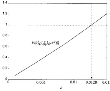
Step 3. In ® gure 2, the supremum of the function

q u~~_{g e}

,

ejµ in the range µ 0

,

2

p

is depicted

with respect toe . According to this ® gure and

the inequality (5.7 a

)

, we havee 3 0.0128.

Step 4. Choosee min e 1

,

e 2

,

e 3 0.0128.

Step 5. Sincee e 3 0.0128, we resort to case (3

)

. In

® gure 3, the supremum of the function

q u~~~_g e

,

ejµ in the range µ 0

,

2

p

is depicted

with respect toe . According to this ® gure and

the inequality (5.7 b), ~_{e 3 0.007 is obtained.}

Since~e 3>e 3, we stop.

According to the above discussion, we conclude that

the discrete time-delay singularly perturbed system (7.1

)

under the composite state feedback control (5.5) with

the state feedback gains obtained in Step 1 and Step 2

is D(0.3, 0.46)-stable for alle <e 0.0128.

8. Conclusion

In this paper, we investigate the D-stabilization problem of a discrete multiple time-delay singularly per-turbed system. Two cases of a new robust D-stability criterion in terms of complex stability radius are ® rst proposed for discrete uncertain multiple time-delay

systems. One is a direct test (i.e. d1< ds

)

and the other

is a boundary test. Then, the corresponding slow and Figure 2. The supremum of the functionq u~_g~ _e

,

ejµ in the

rangeµ 0

,

2p .

Figure 3. The supremum of the functionq u~~_g~ e

,

ejµ in the

rangeµ 0

,

2p .

² In this example, the Euclidean norm is considered.

fast subsystems of a discrete multiple time-delay singu-larly perturbed system are derived by using the tech-nique of time-scale separation. the state feedback controls for the D-stabilization of the slow and fast sub-systems are separately designed, and a composite state feedback control for the original system is subsequently synthesized from these state feedback controls.

There-after, a frequency domain e -dependent D-stability

cri-terion is proposed for the original discrete multiple time-delay singularly perturbed system under the composite state feedback control. If any one of the conditions of this criterion is ful® lled, the D-stability of the original closed-loop system is thus investigated by establishing that of its corresponding slow and fast closed-loop sub-systems. Finally, an e cient algorithm is proposed to obtain a less conservative D-stability bound of the sin-gular perturbation parameter and to reduce the compu-tation time.

Appendix A. Proof of Theorem 1:

(I): The necessary and su cient condition to guarantee

that all poles of the system (2.1) lie inside the speci® c

disk D

a

,

r is that all solutions of the characteristic

equation

det zI A D A n

i 1

Adi D Adi z hi 0

A 1

satisfy z

a

< r. Let z

a

/r be replaced by a

vari-able g (i.e. z rg

a

; then (A 1)becomes

det rg a I A D A n i 1 Adi D Adi rg a hi 0 or, equivalently, det gI A a I r 1 r D A n i 1 Adi D Adi rg a hi 0 A 2

If g 1, we have r

a

rg

a

. From equation

(2.7 a

), the following inequality (A 3)

can be achieved:

1 r D A n i 1 Adi D Adi rg

a

hi <q A

a

I r for g 1 A 3 1 r D A n i 1 Adi D Adi rg

a

hi <q A

a

I r for g 1 A 4

Since all the eigenvalues of A are within the disk D

a

,

r ,

all the eigenvalues of A

a

I /r lie inside the unit circle.

Hence, from (A 4)and Lemma 1, all eigenvalues of the

matrix A

a

I r 1 r D A n i 1 Adi D Adi rg

a

hi A 5

remain inside the unit circle for g 1. That is,

¸ A

a

I r 1 r D A n i 1 Adi D Adi rg

a

hi <1 for g 1 A 6 This implies that

g ¸ A

a

I r 1 r D A n i 1 Adi D Adi rg

a

hi for g 1 A 7

In view of (A 7), all solutions of the characteristic

equa-tion (A 2)satisfy g < 1 (i.e. z

a

/r < 1 . This

com-pletes the proof of case (I).

(II): If the system (2.1)is not D

a

,

r -stable, then there

exists a solution_{g of the characteristic equation (A 2}^

₎

satisfying ^ g ¸ A a I r 1r D A n i 1 Adi D Adi rg^ a hi 1 A 8

On the basis of Lemma 1 and equation (A 8

)

, the

follow-ing inequality is obtained: 1 r D A n i 1 Adi D Adi rg^

a

hi q A _r

a

I A 9 Since 1 r D A n i 1 Adi D Adi rg^

a

hi 1 r b n i 1 Adi rg^

a

hi n i 1

h

i r

a

hi 1 r b n i 1 Adi

h

i r

a

hi A 10 we have

ds q A _r

a

I 1_r D A n i 1 Adi D Adi rg

a

hi 1 r b n i 1Adi rg

a

hi n i 1h i r

a

hi _{h g} 1 r b n i 1 Adi h i r

a

hi d1 f or g 1 A 11 Moreover, according to (A 8), we can obtain the follow-ing inequality: 1 _g^ _¸ A a I r 1 r D A n i 1 Adi D Adi rg^ a hi A a I r 1 r D A n i 1 Adi D Adi rg^ a hi A a I r 1 r b n i 1 Adi h i r a hi d1r A 12

This implies that, if the system (2.1)is not D

a

,

r -stable,

then all the unstable poles of this system must be within

the bounded region U1. Hence, if the inequality (A 11

)

is

not true (i.e. h g does not lie inside the interval ds

,

d1

)

for all g U1, then the system (2.1)is robustly D

a

,

r

-stable. This completes the proof of case (II

)

.

Appendix B. Proof of Theorem 2:

(I): Applying a z-transform to the closed-loop system

(5.6)yields zX1z n i 0 M1iz hiX1 z n i 0 M2iz hiX2 z xz1 0 B1a zX2z n i 0 M3iz hiX1 z n i 0 M4iz hiX2 z xz2 0 B1b

in which x10 and x2 0 are the bounded initial

con-ditions of the states x1k and x2 k , respectively.

According to (B1b), we have X2z zI n i 0 M4iz hi 1 _n i 0 M3iz hi X1 z z zI n i 0 M4iz hi 1 x20 B2

Substituting (B2

)

into (B1a

)

, X1z is obtained as

X1 z zU 1 z n i 0 M2iz hi zI n i 0 M4iz hi 1 x2 0 zU 1 z x₁ 0 B3 where U z zI n i 0 M1zz hi n i 0 M2iz hi zI n i 0 M4iz hi 1 _n i 0 M3iz hi B4

Since the fast closed-loop subsystem (4.9) is D

a

,

r

-stable, and the basis of the fact that M4i D fi² , all

poles of the term

zI n

i 0

M4iz hi 1

in (B3

)

lie inside the disk D

a

,

r . Moreover, all poles of

the term ni 0M2iz hi in (B3) are z 0 which is also

inside the disk D

a

,

r { r >

a

. Therefore, to let all

poles of X1 z be within the disk D

a

,

r and likewise

those of X2 z , we need only to ® nd the condition which

guarantees that all the poles of U 1z are within the

disk D

a

,

r . Substituting (5.5 b

)

and (5.6 c) into (B4),

we have U z zI n i 0 A 1i B1k1i z hi n i 0 M 2iz hi zI n i 0 M4iz hi 1 _n i 0 M3iz hi zI n i 0 A1i B1 ksi e kfi I e n j 0 ~ A2j 1 n j 0A2j B2 n j 0ksj z hi n i 0m2iz hi

² The fact that M4i D Afican be observed by comparing

(4.9 b)with (5.6 c)and using the matrices de® ned in (3.7 b)and (5.5 c).

zI n i 0 M4iz hi 1 _n i 0 M3iz hi zI n i 0 A1i e n j 0 ~ A1j I e n j 0 ~ A2j 1 A2i B1 e n j 0 ~ A1j I e n j 0 ~ A2j 1 B2 ksi z hi n i 0 e n j 0 ~ A1j I e n j 0 ~ A2j 1 A2i B2ksi z hi n i 0 e B1kfi I e n j 0 ~ A2j 1 n j 0A2j B2 n j 0ksj z hi n i 0 M2iz hi zI n i 0 M4iz hi 1 _n i 0 M3iz hi zI n i 0 Asi Bsksi z hi R z n i 0 M2iz hi zI n i 0 M4iz hi 1 _n i 0 M3iz hi see 3.5 b and 3.5 c K z I K 1z R z n i 0 M 2iz hi zI n i 0 M4iz hi 1 _n i 0 M3iz hi where K z zI n i 0 Asi Bsksi z hi and R z n i 0 e n j 0 ~ A1j I e n j 0 ~ A2j 1 A2i B2ksi e B1kfi I e n j 0 ~ A2j 1 n j 0 A2j B2ksj z hi Hence, we have U 1 z I u z 1K 1 z w 1 zK 1 z B5 where w z I u z with u z K 1 z R z n i 0 M2iz hi zI n i 0 M4iz hi 1 _n i 0M3iz hi

Since the slow closed-loop system (4.2

)

is D

a

,

r -stable,

the termK 1z in (B5

)

has all poles lying inside the disk

D

a

,

r . Consequently, if all poles of the term

w 1 z I u z 1 in (B5

)

lie inside the disk

D

a

,

r , we can guarantee that U 1 z has all poles

lying inside the disk D

a

,

r .

Let z

a

/r be replaced by a variable g (i.e.

z rg

a

; then the termw 1 z becomes

w 1z I u z 1 I u rg

a

1 I u g g 1 w g1 g B6a where u gg K g1g Rg g n i 0 M2i rg

a

hi rg

a

I n i 0 M4i rg

a

hi 1 n i 0 M3i rg

a

hi B6b with K gg rg

a

I n i 0 Asi Bsksi rg

a

hi and Rg g n i 0 e n j 0 ~ A1j I e n j 0 ~ A2j 1 A2i B2ksi e B1kfi I e n j 0 ~ A2j 1 n j 0 A2j B2ksj rg

a

hi

If the following inequality holds:

detw g g det I u g g > 0 g 1 B7

(i.e. all the poles ofw g1 g are within the unit disk

), then

all the poles of w 1z lie inside the disk D

a

,

r . Let

g ~g 1; thenw s g becomes w gg w g ~g 1 I u g ~g 1 I u~~_g ~g _w~~_g ~g B8a where ~ u ~_g ~g ~K _g~1 g~ R~_g~ ~g n i 0 M2i r~g 1

a

hi r~_g 1

_a

_I n i 0 M4i r~g 1

a

hi 1 n i 0 M3i r~g 1

a

hi B8b with ~ K ~_g ~g rg~ 1

a

I n i 0 Asi Bsksi rg~ 1

a

hi and ~ R~_g ~g n i 0 e n j 0 ~ A1j I e n j 0 ~ A2j 1 A2i B2ksi e B1kfi I e n j 0 ~ A2j 1 n j 0 A2j B2ksj r~g 1

a

hi

Therefore, the examination of (B7

)

is equivalent to

investigating the following inequality:

detw~~_g ~g det I _u~~_g g > 0~ ~g 1 B9

Introducing the singular perturbation parametere into

(B8b

)

,u~~_g ~g can then be rewritten as ~ u _g~ _e

,

~g ~_K ~_g1 _e

,

~g R~~_{g e}

,

g~ n i 0 M2i e r~g 1

a

hi r~_g 1

_a

_I n i 0 M4i e r~g 1

a

hi 1 n i 0 M3i e r~g 1

a

hi B 10 with ~ K ~_g e

,

~g r~g 1

a

I n i 0 Asi e Bs e ksi r~g 1

a

hi and ~ R~_g e

,

~g n i 0 e n j 0 ~ A1j I e n j 0 ~ A2j 1 A2i B2ksi e B1kfi I e n j 0 ~ A2j 1 _n j 0A2j B2ksj rg~ 1

a

hi

Since all poles of the term zI ni 0M4iz hi 1in (B3

)

and the termK 1 z in (B5

)

lie inside the disk D

a

,

r ,

the terms rg

a

I ni 0M4i rg

a

hi 1 and

K _g1 g in (B6b

)

do not have any pole lying inside the

region g 1. Moreover, the term Rg g in (B6b

)

does

not have any pole lying inside the region g 1 ({ the

multiple poles of Rg g are at g

a

/r and r >

a

)

either. We can then conclude that u gg does not have

any pole lying inside the region g_~ 1. Consequently,

u ~_g e

,

~g u~~_g ~g u g ~g 1 has no poles lying inside the

region ~_{g 1 and the function ¸iu}~_~ge

,

~_{g ² is hence}

analytic and continuous in the bounded domain ~ g 1. Therefore, if (5.7 a)holds, i.e. s u~~_ge

,

~g max i ¸i ~ u ~_{g e}

,

g < 1~ ~g 1 B11

then we have (according to Lemma 4

)

s u~~_ge

,

~g < 1 ~g 1 B12

On the basis of (B12

)

and Lemma 3, the following

inequality is obtained:

detw~~_g ~g det I u~_g~ ~g det I u~~_g e

,

~g > 0

~

g 1 B13

and then the inequality (B9), or equivalently (B7), is

ful® lled. This implies that the closed-loop system (5.6

)

is stable, thus completing the proof of case (I).

(II): Using the matrix inversion formula

I R P 1 I R I PR 1P B14

the functionw 1 z in (B5

)

can be rewritten as

² The notation¸i A denotes the eigenvalue of the matrix A.