Consistency of Breast Density Measured from the Same Women in Four
Different MR Scanners
Jeon-Hor Chen1,2,3 , Siwa Chan4, Yi-Jui Liu5, Dah-Cherng Yeh6, Chin-Kai Chang2, Li-Kuang Chen1, Wei-Fan Pan2, Chih-Chen Kuo2, Muqing Lin1, Daniel H.E. Chang1, Peter T. Fwu1,Min-Ying Su1
1Tu & Yuen Center for Functional Onco-Imaging of Department of Radiological Science, University of California Irvine, California, United States
2Department of Radiology, China Medical University Hospital, Taichung, Taiwan
3Department of Medicine, School of Medicine, China Medical University, Taichung, Taiwan 4Department of Radiology, Taichung Veterans General Hospital, Taichung, Taiwan
5Department of Automatic Control Engineering, Feng Chia University Taichung, Taiwan 6Department of Surgery, Taichung Veterans General Hospital, Taichung, Taiwan
Running Title: Breast Density Measured in Different MR Scanners
Corresponding Author: Jeon-Hor Chen, M.D.
No. 164, Irvine Hall, Tu & Yuen Center for Functional Onco-Imaging, University of California, Irvine, CA92697
(Tel): 949-824-9327; (Fax): 949-824-3481, e-mail: [email protected]
Acknowledgement: This work was supported in part by NIH/NCI Grant No. R01 CA127927 and R03 CA136071.
Consistency of Breast Density Measured from the Same Women in Four
Different MR Scanners
ABSTRACT
Purpose: To compare the breast volume (BV), fibroglandular tissue volume (FV) and percent density (PD) measured from breast MRI of the same women using four different MR scanners. Methods: The study was performed in 34 healthy Asian volunteers using two 1.5T (GE and Siemens) and two 3T (GE and Philips) MR scanners. The BV, FV, and PD were measured on non-fat-suppressed T1-weighted images using a comprehensive computer algorithm-based segmentation method. The scanner-to-scanner measurement difference, and the Coefficient of Variation (CV) among the four scanners were calculated. The measurement variation between two density morphological patterns presenting as the central type and the intermingled type was separately analyzed and compared.
Results: All four scanners provided satisfactory image quality allowing for successful completion of the segmentation processes. The measured parameters between each pair of MR scanners were highly correlated, with R2 ≥ 0.95 for BV, R2 ≥ 0.99 for FV, and R2 ≥ 0.97 for PD in all comparisons. The mean percent differences between each pair of scanners were 5.9-7.8% for BV, 5.3-6.5% for FV, 4.3-7.3% for PD; with the overall CV of 5.8% for BV, 4.8% for FV, and 4.9% for PD. The variation of FV was smaller in the central type than in the intermingled type (p=0.04).
Conclusions: The results showed that the variation of FV and PD measured from 4 different MR scanners are around 5%, suggesting the parameters measured using different scanners can be used for a combined analysis in a multi-center study.
I. INTRODUCTION
Many mammography studies have shown that mammographic density is a strong independent risk factor for development of breast cancer.1-3 Based on this evidence the Breast Cancer Preventive Collaboration Group has recommended that mammographic density should be considered in the risk prediction model4; however, so far it has not been incorporated into any commonly used models. One main issue that needs to be resolved is how to obtain reliable quantitative density measures. This is a very important research area currently under rigorous investigation in the breast density research community. Due to its two dimensional nature, mammographic density bears the intrinsic limitation of tissue overlapping, and cannot provide a true volumetric measure. Also, the measured density is susceptible to many sources of technical and positioning variations.5 Other methods that can measure quantitative breast density have been developed and evaluated; including volumetric measurements made based on 3D MRI.6-15 However, so far there have not been published results demonstrating the association between MRI-based density parameters and cancer risk.
Currently, breast MRI is recommended to be performed at 1.5T. The current guideline from the American Cancer Society recommends screening MRI to be performed on women with a lifetime risk greater than 20%, thus only limited cases can be collected from a single site. For assessing the association between MRI-based density and cancer risk, a large dataset is required, and combining MRI from multiple centers is the only feasible way to achieve this goal. Because different scanners and different imaging protocols are used at different institutions, that will lead to intrinsic
differences in the acquired image quality and influence the segmented density parameters. Thus, as the first step, whether or how the densities measured from different centers can be combined needs to be investigated.
Although 3T MRI is able to provide images of higher signal-to-noise ratio and higher spatial resolution16, the higher field inhomogeneity may compromise the image quality.17-19 Nevertheless,
due to the wide availability of 3T MRI scanners, many clinical breast MRI studies are also done at 3T. The purpose of this preliminary work is to compare the measurement consistency in breast volume (BV), fibroglandular tissue volume (FV) and percent density (PD) using 4 different scanners, two at 1.5T and two at 3T. The percent difference between the parameters measured by each pair of different scanners is calculated; also the overall variation among the 4 scanners was evaluated using the coefficient of variation. In addition, we also evaluated whether the amount of dense tissues and different breast density morphological types will affect the consistency of
measurement. Based on the relative distribution pattern of fibroglandular tissue and fatty tissue, the breast is categorized as the central type (dense tissue inside surrounded by fatty tissue outside) or the intermingled type (with mixed dense tissue and fatty tissue), and the measurement variation between these two types was compared.
II. MATERIALS AND METHODS II.A. Subjects
This study was approved by the Institutional Review Board and was HIPAA-compliant. All subjects provided written informed consent. Thirty-four healthy Asian female subjects (age 20-64, mean 35 y/o, 26 pre-menopausal and 8 post-menopausal) were recruited to receive non-contrast breast MRI studies at 4 different MR scanners, including GE Signa-HDx 1.5T and GE Signa-HDx 3T (GE Healthcare, Milwaukee, WI), Siemens Symphony 1.5T TIM (Siemens, Erlangen, Germany), and Philips Achieva 3.0T TX (Philips Medical Systems, Eindhoven, Netherlands). None of these 34 subjects had been diagnosed with histological-confirmed breast diseases. At the time of participation in this study they were all healthy without any breast related symptoms. The pre-menopausal
taking contraceptive pills. Three post-menopausal women had a history of taking hormonal
replacement therapy due to post-menopausal syndromes, but the treatment was ceased long before (> 1 year) participating in this study.
II.B. MR imaging studies
The 4 MR scans for each subject were performed at two different medical institutions in the same city, 6 miles apart, and were completed within 2 days to reduce the biological effect due to endogenous hormonal fluctuation. Prior to the study, the T1W imaging sequences for breast segmentation were tested with the assistance of clinical application scientists from each vendor to ensure the imaging quality was good enough for breast segmentation. The subjects were in prone position with arms beside the head in the GE 1.5T, GE 3T and Philips 3T studies, but positioned beside the body in the Siemens 1.5T study.
In this study the MR scans were performed bilaterally in axial sections. Since the purpose of this study was to compare the results of breast segmentation, only the 2D fast spin echo (FSE) non-fat-suppressed (or, non-fat-sat) T1 weighted images were acquired and analyzed in all four scanners; and the imaging parameters selected might not be fully comparable with the current clinical MRI standard. For GE 1.5T scanner, an eight-channel breast coil was used, with TR/TE= 607/9 msec, slice thickness= 2mm, slice gap=0, phase-encoding R-L, bandwidth per pixel= 130 Hz, field of view (FOV)=380mm, number of signal average = 2, and imaging matrix= 256x192. For GE 3.0T scanner, an eight-channel breast coil was used, with TR/TE= 650/9 msec, slice thickness= 2mm, slice gap=0, phase encoding R-L, bandwidth per pixel= 217 Hz, FOV=380mm, number of signal average = 2, and imaging matrix= 256x192. For Philips 3.0T scanner, a sixteen-channel breast coil was used. The imaging parameters were: TR/TE= 645/9.0 msec, parallel imaging with SENSE factor = 2, slice thickness= 2mm, slice gap=0, phase encoding R-L, bandwidth per pixel= 174 Hz, FOV=330mm,
number of signal average = 1, and imaging matrix= 328x384. For Siemens 1.5T scanner, a four-channel breast coil was used. The imaging parameters were: TR/TE= 650/9.8 msec, parallel imaging with SENSE factor = 2, slice thickness= 2mm, slice gap=0, phase encoding R-L, bandwidth per pixel= 181 Hz, FOV=330mm, number of signal average = 1, and imaging matrix= 330x384
(660x768 with interpolation). The imaging time of the four scanners was from 2 minutes 50 seconds to 4 minutes 8 seconds.
II.C. Breast and fibroglandular tissue segmentation
The breast and fibroglandular tissue segmentation was performed using a modified published method 14, 20 by a research assistant (CKC) with background of radiological technology and medical imaging and one year of experience in segmenting breast MR images. The four sets of T1W images of the same subject acquired using four different MR scanners were analyzed within two days, to ensure that the operator used the same body landmarks to segment the breast boundary and used the same standard to segment the fibroglandular tissue from the fatty tissue. The order of analysis among the four sets of images was randomly arranged from subject to subject. Before the segmentation, the operator viewed the whole axial T1W images dataset and determined the superior and inferior boundaries of the breast (the beginning and ending slices) by comparing the thickness of breast fat with the body fat. Non-breast subcutaneous fat on the chest typically displays homogenous thickness across the chest wall, and that was used to determine where the breast starts and ends.
The breast segmentation procedures consisted of: 1) Perform an initial horizontal line cut to exclude thoracic region. Depending on the morphology of the breast, a horizontal line was drawn along the posterior margin of each individual subject’s sternum. If some fibroglandular tissues were chopped off, the horizontal line was lowered, up to 35 millimeters posterior from the original sternum landmark. This was to ensure that the breast region analyzed from the four scanners was
consistent, and that the entire fibroglandular tissue was contained within the segmented breast. 2) Apply Fuzzy-C-Means (FCM) clustering21 and b-spline curve fitting 22to obtain the breast-chest boundary. In this step, the operator checked each slice and determined if the pectoralis muscle has been removed adequately. If not, the operator had to modify the boundary manually. 3) A novel method based on nonparametric nonuniformity normalization (N3) and adaptive FCM algorithm20 was used to remove the strong intensity non-uniformity and correct the bias field for segmentation of fibroglandular tissue and fatty tissue. The N3 algorithm is a fully automatic histogram-based
method, and is a popular correction method widely used in the literature.23 The N3 algorithm is able to reduce the bias field while avoiding the problem of generating erroneous contrast. 4) Apply dynamic searching to exclude the skin along the breast boundary. 5) The standard FCM algorithm is applied to classify all pixels on the image. The default setting is to use a total of 6 clusters, 3 for fibroglandular tissue and 3 for fatty tissues. After completing the process, the dense tissue ROI is mapped onto the original MRI and the operator went through the images slice by slice to inspect the segmentation quality by comparing the segmented images with the original non-segmented images. If the quality analyzed using this setting is not satisfactory, the operator can choose to use a different cluster number, typically by decreasing the total cluster number from 6 to 5, with 2 or 3 clusters as the dense tissue. Figures 1 to 3 show fibroglandular tissue segmentation in three subjects.
Finally, after completing the segmentation and verification processes, a vertical line between the breasts perpendicular to the sternum was drawn to separate the left and the right breasts. Then, the quantitative BV, FV, and PD which was calculated as the ratio of FV over BV x100%, were obtained. The processing time to analyze the whole set of images for both breasts of a subject, including the corrections, can be completed in 45 minutes.
The MR breast morphology was determined by an experienced radiologist (JHC) based on the definition used in a previous study.24 Briefly, when the fibroglandular tissue of the breast was centrally located and was well-surrounded by the fatty tissue, the breast was defined as a central type breast (Figure 2 and Figure 3). On the contrary, when the fibroglandular tissue and the fatty tissue were mixed together in the whole breast, it was defined as the intermingled breast morphology (Figure 1). Of the 34 subjects, 17 were central type, and 17 were intermingled breast morphology; therefore, there were a total of 34 central type breasts and 34 intermingled type breasts.
II.E. Statistical methods
The statistical analyses were performed using 68 breasts from 34 subjects. First, the parameters measured between each pair of MR scanners were compared. A total of 6 comparisons were made: namely GE 1.5T vs. GE 3.0T, GE 1.5T vs. Philips 3.0T, GE 1.5T vs. Siemens 1.5T, GE 3.0T vs. Philips 3.0T, GE 3.0T vs. Siemens 1.5T, Philips 3.0T vs. Siemens 1.5T. In each paired comparison, the Pearson’s correlation was used to evaluate the overall correlation from all 68 breasts. To
evaluate the level of uncertainty of the correlation between pairs of MR systems, we further analyzed the confidence interval of the correlation using the statistical analysis function (Matlab, version 7.11.0). The data was fitted by finding the coefficient of a polynomial of degree 1 in the least square sense. The norm of residuals was the sum of the squares of the differences between the predicted values and the actual values, which represented the level of correlation, the smaller number the closer correlation.
For each breast, the absolute difference in the measured parameters from two scanners was calculated, and the percent difference was calculated as the absolute difference over their mean value (x 100%). The mean±stdev, as well as the range, of the difference calculated from all 68 breasts was evaluated. In addition, the overall consistency of the measured parameters among the four scanners
was compared based on the coefficient of variation (CV), defined as the standard deviation from the four measurements divided by their mean value (x100%). A higher CV indicated a larger
measurement variation. The CV measured in the central type and the intermingled type breast was compared using the two-tailed student t test, using p < 0.05 as the significance level. Lastly, in order to evaluate the relationship between the measurement variation with the amount of density, the 68 breasts were separated into 4 quartiles based on their FV values, 17 breasts in each quartile group, and the measurement CV between them was compared.
III. RESULTS
III.A. Measurement variation between each pair of four MR scanners
All four scanners provided satisfactory image quality for successfully completing the
segmentation processes. Contrast between the fibroglandular tissue and the fatty tissue is high, as demonstrated in Figures 1 to 3. Table 1 shows the mean value of BV, FV, and PD calculated from 68 breasts using each scanner. Figures 4 to 6 show the correlation of BV, FV, and PD between each pair of two MR scanners, with R2 = 0.99 in all 6 comparisons for FV. For BV, the R2 in 6 comparisons are 0.95, 0.96, 0.97, 0.98, 0.98, 0.99, which shows that the correlation was worse than that for FV. The result indicates that there is a higher variation in the segmentation of breast from the body; but as long as the fibroglandular tissue is fully contained within the segmented breast, the measurement of FV is consistent. Figure 7 shows the level of uncertainty in each pair of comparison for PD. It was obvious that the correlation was better between any pair of 1.5T GE, 3.0T GE, and 3.0T Philips (all norm residuals numbers <13) than when Siemens was compared with any one of the three other MR scanners (norm residuals > 16). The scanner-to-scanner paired t-test, however, did not show any significant difference for any analyzed parameter. Table 2 shows the mean value and the range of the
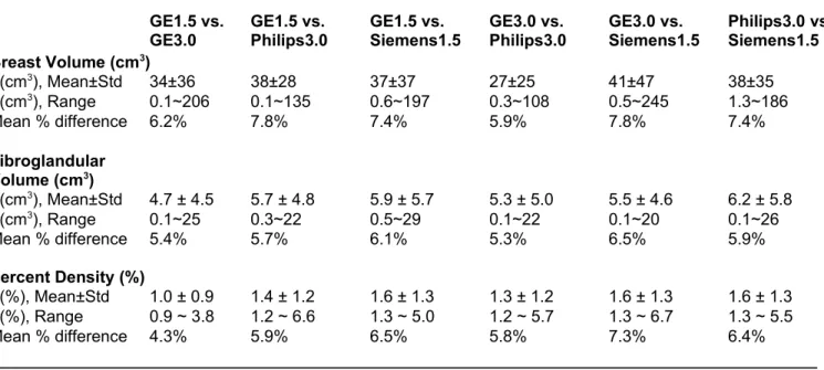
absolute difference in the measured BV, FV, and PD, as well as the mean percent difference for each paired comparison. The mean percent differences in the 6 paired comparisons ranged from 5.9-7.8% for BV, 5.3-6.5% for FV, 4.3-7.3% for PD. The ranges were comparable in all 6 paired comparisons, and there was not a systematic difference from any particular scanner(s).
III.B. Coefficient of variation in all breasts and the central and intermingled morphological types
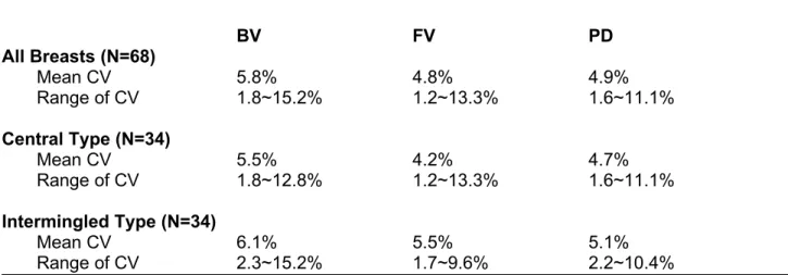
The overall measurement variation from 4 scanners is evaluated using the coefficient of variation (CV), listed in Table 3. The CV was higher for BV (5.8%) than that for FV (4.8%) or PD (4.9%). Among the 68 analyzed breasts, CV higher than 10% was found in BV of 5 breasts, but only in FV of 2 breasts and PD of one breast. In central vs. intermingled type comparison, the mean CV for measurement of FV was 4.2% for the central type, which was significantly lower compared to 5.5% for the intermingled type (p=0.04). The mean CV for BV was 5.5% for the central type and 6.1% for the intermingled type, not significantly different (p=0.3). The mean CV for PD was 4.7% for the central type and 5.1% for the intermingled type, not significant either (p=0.3).
III.C. Coefficient of variation in four quartile groups based on FV values
The 68 breasts were separated into 4 quartiles based on their FV values, with 17 breasts in each group. The mean value and the range of FV were: 48.2 (28.9~59.9) cm3 in the first quartile; 66.9 (60.4~75.7) cm3 in the second quartile; 110.7 (78.4~144.9) cm3 in the third quartile; and 234.9 (145.8~368) cm3 in the 4th quartile. The coefficient of variation for FV was 2.9% in the 4th quartile group, which was significant smaller compared to the 5.5% in the first quartile (p=0.001), 5.0% in the second quartile (p=0.008), and 5.0% in the third quartile (p=0.005). The smaller CV in the 4th
quartile was due to their much higher mean FV value, so the results did not suggest an obvious trend of measurement variation related to different amount of fibroglandular tissues.
IV. DISCUSSION
Quantitative 3D MR-based analysis of breast density can potentially provide an imaging biomarker for assessing cancer risk or predicting therapeutic efficacy of hormonal treatments. MRI provides detailed 3D distribution of fibroglandular tissue not subject to the tissue-overlapping problem as in mammography, and thus is suitable for volumetric measurements. We have developed a comprehensive computer algorithm-based segmentation method for quantitative analysis of whole BV and FV on 3D MRI14, 20, which has shown both intra- and inter-operator variation smaller than 5%. The method has been applied to study the age- and race-related differences 25, as well as the change in patients receiving chemotherapy 26 and tamoxifen.27 The variation coming from the operator(s) is one major concern, which can be solved by minimizing the interventions that need to be provided by the operator. During the past several years we have been continuing to improve the robustness of method by standardizing the processes. For segmentation of the breast, using easily recognizable body landmarks such as sternum can minimize the judgment call from different operators. For the segmentation of fibroglandular tissue, one important step is to implement a
powerful bias field correction method that can work in a large imaging field, and we have shown that the N3+FCM and the coherent local intensity clustering (CLIC) algorithm both worked very well.20 Then, within a homogeneous intensity field, it is possible to fix the number of FCM clusters used for segmentation of fibroglandular tissue. We have evaluated several different combinations, and decided to choose a total of 6 clusters as the default setting, 3 for fibroglandular and 3 for fatty tissues. Before MRI-based breast density can be used as a reliable imaging biomarker, it is necessary to thoroughly evaluate the dependence of the measured parameters on possible biological and
technical factors. In addition to evaluating operator variations, we have recently reported the biological fluctuation of the measured density associated with the change of endogenous hormone during a menstrual cycle.28 In another study we investigated the variation of parameters analyzed based on fat-sat and non-fat-sat images.29
In the present study, we set out to investigate another very important technical factor that may affect the measured density parameter- the use of different MR scanners. This is particularly important for combining data obtained from different performance sites that use different MR scanners. In order to facilitate such a multi-center study, the consistency of data measured from different sites should be verified.30 The optimal design is to have the same subject receive repeated examinations using different scanners. The Alzheimer's Disease NeuroImaging Initiative (ADNI) 31-33 has diligently arranged “traveling volunteers” to receive brain MRI using optimized imaging protocol across all sites.33 Similarly, in this study we recruited 34 healthy women to receive breast MRI study using four different MR scanners located at two near-by medical institutions in the same city. In order to minimize the biological variations such as that coming from the endogenous
hormone, the four studies were completed within two days.
We chose to use four scanners from three major manufacturers, GE 1.5T and GE 3.0T, Siemens 1.5T, and Philips 3.0T. These scanners were equipped with the state-of-the-art breast coil and
imaging sequences. The non-fat-sat T1-weighted images acquired using Fast Spin Echo (FSE) pulse sequence were used for the analysis. This sequence was chosen because of the high image quality and a good tissue contrast between the fibroglandular tissue and the fatty tissue. The quality of MR images depends on the homogeneity of the B0 field, the B1 transmit field of the body RF coil, and the receiver profile of the surface breast coil. 3T MR offers a higher signal-to-noise ratio than 1.5T 34, but it comes with technical problems that may offset the benefits. B0 field is usually
without fat-sat. B1 field may lead to spatial variations of the delivered radiofrequency pulses (or, non-uniform flip angle) in a large FOV, which thenaffects signal intensity.35 The variation of the B1 transmission is higher at 3T compared to 1.5T. Compared with the B0 field strengths and
inhomogeneity and the B1 transmission inhomogeneity, the different receiver surface breast coil is probably the biggest source of variations. The types of coils, manufacturers, models, and number of elements will affect the quality of breast MR images. The strong bias field presents a difficulty for thresholding- or clustering-based segmentation approaches. Although we have shown that our N3+FCM method20 worked well, sometimes a local contrast adjustment is still needed, and there is room for further improvements. Along the same line of research, Kruggel et al. reported the
difference in the segmented gray matter and white matter in a large ADNI brain MRI dataset acquired using 17 different MR scanner models from all three major manufacturers.36 Despite the standardized protocol, differences across scanners were considerable.It was concluded that two most likely factors contributing to the different segmentation results are scanner-dependent geometrical inaccuracies and differences in the tissue contrast.36
In this study, the pulse sequences were tested with the assistance of clinical application
scientists from each vendor to ensure satisfactory imaging quality prior to the MR examinations. The measurement variation (CV) of BV, FV, and PD among the four different scanners was 5.8%, 4.8% and 4.9% respectively, which fell in the range of operator variation and positional difference of approximately 5% using the same scanner.14
For measurement of BV, we used the sternum as the body landmark for determining the posterior boundary of the breast. Although this was easily identifiable, some fibroglandular tissue extending into the axilla might be chopped off. This problem was commonly encountered in our cohort of Asian women who have relatively dense breasts. If this happened, the operator needed to lower the horizontal cutting line 5-35mm posterior to the sternum to ensure that all fibroglandular
tissue was included in the segmented breast. When a shift was used, the same shift was used in the analyses of this subject’s 4 datasets, so the same criteria were applied. Ensuring that all
fibroglandular tissue was contained within the segmented breast helped in minimizing the
measurement variation of FV and PD (CV from 4 scanners 4.8% and 4.9%, respectively). The CV for BV (5.8%) was slightly higher compared to FV and PD. Also, among the 68 analyzed breasts, CV higher than 10% was found in BV of 5 breasts but only occurred in FV of 2 breasts and PD of one breast. A higher variation in BV was likely due to the uncertainty in the determination of the beginning and ending slices. This may change with different body and arm positioning, and thus cannot be fixed. Since the breast tissue in the starting and ending slices is mainly fatty tissue, this uncertainty will not affect the measurement of FV as much. In the 5 breasts showing CV of BV higher than 10%, it was mainly because the BV measured by one scanner was much different compared to the other three scanners. In the case shown in Figure 3, the BV of both breasts measured by GE 3.0T was smaller compared to the others, and in another subject the BV of both breasts measured by Siemens 1.5T was much smaller. However, the difference was not consistently coming from one particular scanner, thus there was not a noticeable systematic difference in the measurement of BV. For the correlation of PD between each pair of MR scanners, the level of uncertainty became more obvious when the Siemens scanner was compared with any one of the three other scanners (Figure 7). It was postulated that the difference of arm position (arms beside the head in the GE 1.5T, GE 3T and Philips 3T studies, but arms beside the body in the Siemens 1.5T study) may partially account for the results.
The variation in the measurement of FV was more likely coming from the different tissue contrast and the partial volume effect, which was associated with the density morphological types and the spatial resolution. In this study, the spatial resolution along the read-out direction of the Philips 3.0T and Siemens 1.5T (acquisition matrix 328x384 and 330x384) was higher than that of
the GE 1.5T and GE 3.0T (acquisition matrix 256x192), but we did not observe systematic differences in the measured parameters between these scanners. We further investigated whether different breast morphologies would affect the measurement consistency, and found that the central type breast tended to have more consistent measurement of the FV than the intermingled type (p=0.04). As seen in the three case examples shown in Figures 1 to 3, the partial volume effect is clearly noted in the intermingled type; and in contrast, the signal intensity is more homogeneous in the central type. Nonetheless, the measurement variation for the intermingled type can be managed well by using a consistent FCM clustering method, as seen in the case shown in Figure 1 that has the overall measurement CV of 5.6% for BV, 4.6% for FV, and 4.6% for PD. We also evaluated the variation in breasts with different amount of fibroglandular tissues. A lower CV was found in the 4th quartile group with the highest FV volume, which was very likely coming from its high mean value that makes the CV small. Therefore, we did not observe a trend of measurement variation with respect to the amount of fibroglandular tissues. We have inspected the results from all 68 breasts using 4 scanners, and as the results shown in Table 2, the ranges of CV in all 6 paired comparisons were comparable, and there was not a systematic trend related to a specific scanner that could explain the high variations observed in some subjects. Therefore, the degree of variations presented in this study is very likely representing the natural variations coming from both the technical and the biological sources that will be encountered in a typical breast MRI study.
This study had several limitations. The sample size was small. The subjects were Asian women with small and dense breasts, thus the results may not be generalized to other populations.
Specifically, for women who have very fatty breasts with only scarce fibroglandular tissue, the measurement of FV may be more severely affected by the partial volume effect, and the percent variation will be higher due to the small denominator. Unfortunately in this study we did not include women with very fatty breast to investigate its effect. We only had 8 post-menopausal women, and
they still had relatively dense breasts. Variations of the different scanners, including the scanners per se, the sequences/scan parameters used, and the gradient non-linearity, can directly affect the quality of the breast segmentation. The variation of matrix choices among scanners in this study might introduce some unnecessary variation in segmented volume results. For the 2 GE scanners, with a FOV of 38cm and 256 x 192 matrix, the spatial resolution is less than that clinically acceptable for ACR Breast MRI Accreditation. Our previous study29, with a matrix size of 480x480mm and FOV=31–38 cm, however, has shown that FV measured on downsampled images (240x240) only showed a small (<5%) difference.
CONCLUSION
The results from this pilot study show that when a well-developed segmentation method is used, consistent density parameters from the same women can be obtained from images acquired using different MR scanners. It was found that the overall variation was around 5% for the measurements of FV and PD, suggesting that breast density data analyzed from different scanners in multiple centers may be used for a combined analysis.
REFERENCES
1. N. F. Boyd, H. Guo, L. J. Martin, L. Sun, J. Stone, E. Fishell, R. A. Jong, G. Hislop, A. Chiarelli, S. Minkin, and M. J. Yaffe, “Mammographic density and the risk and detection of breast cancer,” N Engl J Med. 356, 227-236 (2007) .
2. V. A. McCormack, and I dos Santos Silva, “Breast density and parenchymal patterns as markers of breast cancer risk: a meta-analysis,” Cancer Epidemiol Biomarkers Prev. 15, 1159-1169 (2006).
3. C. M. Vachon, V. S. Pankratz, C. G. Scott, S. D. Maloney, K. Ghosh, K. R. Brandt, T. Milanese, M. J. Carston, and T. A. Sellers, “Longitudinal trends in mammographic percent density and breast cancer risk,” Cancer Epidemiol Biomarkers Prev. 16, 921-928 (2007). 4. R. J. Santen, N. F. Boyd, R. T. Chlebowski, S. Cummings, J. Cuzick, M. Dowsett, D. Easton, J.
F. Forbes, T. Key, S. E. Hankinson, A. Howell, J. Ingle and Breast Cancer Prevention
Collaborative Group, “Critical assessment of new risk factors for breast cancer: considerations for development of an improved risk prediction model,” Endocr Relat Cancer. 14, 169-187 (2007). Review.
5. J. A. Harvey, and V. E. Bovbjerg, “Quantitative assessment of mammographic breast density: relationship with breast cancer risk,” Radiology. 230, 29-41 (2004).
6. J. Eng-Wong, J. Orzano-Birgani, C. K. Chow, D. Venzon, J. Yao, C. E. Galbo, J. A. Zujewski, and S. Prindiville, “Effect of Raloxifene on mammographic density and breast magnetic resonance imaging in premenopausal women at increased risk for breast cancer,” Cancer Epidemiol Biomarkers Prev. 17, 1696-1701 (2008).
7. M. Khazen, R. Warren, C. Boggis, E. C. Bryant, S. Reed, I. Warsi, L. J. Pointon, G. E. Kwan-Lim, D. Thompson, R. Eeles, D. Easton, D. G. Evans, M. O. Leach, and Collaborators in the United Kingdom Medical Research Council Magnetic Resonance Imaging in Breast Screening
(MARIBS) Study, “A pilot study of compositional analysis of the breast and estimation of breast mammographic density using three-dimensional T1-weighted magnetic resonance imaging,” Cancer Epidemiol Biomarkers Prev. 17, 2268-2274 (2008).
8. J. Wei, H. P. Chan, M. A. Helvie, M. A. Roubidoux, B. Sahiner, L. M. Hadjiiski, C. Zhou, S. Paquerault, T. Chenevert, and M. M. Goodsitt, “Correlation between mammographic density and volumetric fibroglandular tissue estimated on breast MR images,” Med. Phys. 31, 923-942 (2004).
9. S. van Engeland, P. R. Snoeren, H. Huisman, C. Boetes, and N. Karssemeijer, “Volumetric breast density estimation from full-field digital mammograms,” IEEE Trans Med Imaging. 25, 273-282 (2006).
10. N. A. Lee, H. Rusinek, J. Weinreb, R. Chandra, H. Toth, C. Singer, and G. Newstead, “Fatty and fibroglandular tissue volumes in the breasts of women 20-83 years old: comparison of X-ray mammography and computer-assisted MR imaging,” AJR 168, 501-506 (1997).
11. J. Yao, J. A. Zujewski, J. Orzano, S. Prindiville, and C. Chow, “Classification and calculation of breast fibroglandular tissue volume on SPGR fat suppressed MRI,” Med Imag Proc SPIE. 1942-1949 (2005).
12. C. Klifa, J. Carballido-Gamio, L. Wilmes, A. Laprie, C. Lobo, E. Demicco, M. Watkins, J. Shepherd, J. Gibbs, and N. Hylton, “Quantification of breast tissue index from MR data using fuzzy cluster,” Proc IEEE Eng Med Biol Soci. 3, 1667-1670 (2004).
13. C. Klifa, J. Carballido-Gamio, L. Wilmes, A. Laprie, J. Shepherd, J. Gibbs, B. Fan, S.
Noworolski, and N. Hylton, “Magnetic resonance imaging for secondary assessment of breast density in a high-risk cohort,” Magn Reson Imaging. 28, 8-15 (2010).
14. K. Nie, J. H. Chen, S. Chan, M. K. Chau, H. J. Yu, S. Bahri, T. Tseng, O. Nalcioglu, and M. Y. Su, “Development of a quantitative method for analysis of breast density based on
3-Dimensional breast MRI,” Medical Physics. 35, 5253-5262 (2008).
15. D. J. Thompson, M. O. Leach, G. Kwan-Lim, S. A. Gayther, S. J. Ramus, I. Warsi, F. Lennard, M. Khazen, E. Bryant, S. Reed, C. R. Boggis, D. G. Evans, R. A. Eeles, D. F. Easton, R. M. Warren, and UK study of MRI screening for breast cancer in women at high risk (MARIBS), “Assessing the usefulness of a novel MRI-based breast density estimation algorithm in a cohort of women at high genetic risk of breast cancer: the UK MARIBS study,” Breast Cancer Res. 11, R80 (2009).
16. R. Rakow-Penner, B. Daniel, H. Yu, A. Sawyer-Glover, and G. H. Glover, “Relaxation times of breast tissue at 1.5T and 3T measured using IDEAL,” J Magn Reson Imaging. 23, 87-91 (2006). 17. C. K. Kuhl, H. Kooijman, J. Gieseke, and H. H. Schild, “Effect of B1 inhomogeneity on breast
MR imaging at 3.0 T,” Radiology. 244, 929-930 (2007).
18. R. M. Mann, C. K. Kuhl, K. Kinkel, and C. Boetes, “Breast MRI: guidelines from the European Society of Breast Imaging,” Eur Radiol. 18, 1307-1318 (2008).
19. C. A. Azlan, P. D. Giovanni, T. S. Ahearn, S. K. Semple, F. J. Gilbert, and T. W. Redpath, “B1 transmission-field inhomogeneity and enhancement ratio errors in dynamic contrast-enhanced MRI (DCE-MRI) of the breast at 3T,” J Magn Reson Imaging. 31, 234-239 (2010).
20. M. Lin, S. Chan, J. H. Chen, D. Chang, K. Nie, S. T. Chen, C. J. Lin, T. C. Shih, O. Nalcioglu, and M. Y. Su, “A new bias field correction method combining N3 and FCM for improved segmentation of breast density on MRI,” Medical Physics. 38, 5-14 (2011).
21. W. Chen and M. L. Giger, “A fuzzy c-means (FCM) based algorithm for intensity
inhomogeneity correction and segmentation of MR images,” in International Symposium on Biomedical Imaging (ISBI), pp. 1307–1310 (2004).
22. N. A. Lee, H. Rusinek, J. Weinreb, R. Chandra, H. Toth, C. Singer, and G. Newstead, “Fatty and fibroglandular tissue volumes in the breasts of women 20–83 years old: Comparison of X-ray mammography and computer-assisted MR imaging,” AJR, Am. J. Roentgenol. 168, 501–506 (1997).
23. J. G. Sled, A. P. Zijdenbos, and A. C. Evans, “A nonparametric method for automatic correction of intensity nonuniformity in MRI data,” IEEE Trans. Med. Imaging. 17, 87-97 (1998).
24. K. Nie, J. H. Chen, D. Chang, C. C. Hsu, O. Nalcioglu, and M.Y. Su, “Quantitative analysis of breast parenchymal patterns using 3D fibroglandular tissue segmentation based on MRI,” Med. Phys. 37, 217-226 (2010).
25. K. Nie, M. Y. Su, M. K. Chau, S. Chan, H. Nguyen, T. Tseng, Y. Huang, C. E. McLaren, O. Nalcioglu, and J. H. Chen, “Age- and race-dependence of the fibroglandular breast density analyzed on 3D MRI,” Med Phys. 37, 2770-2776 (2010).
26. J. H. Chen, K. Nie, S. Bahri, C. C. Hsu, F. T. Hsu, H. N. Shih, M. Lin, O. Nalcioglu, and M. Y. Su, “MRI evaluation of decrease of breast density in the contralateral normal breast of patients receiving neoadjuvant chemotherapy,” Radiology 255, 44-52 (2010).
27. J. H. Chen, Y. C. Chang, D. Chang, Y. T. Wang, K. Nie, R. F. Chang, O. Nalcioglu, C. S. Huang CS, and M. Y. Su, “Reduction of breast density following tamoxifen treatment evaluated by 3-D MRI: preliminary study,” Magnetic Resonance Imaging. 29, 91-98 (2011).
28. S. Chan, M. Y. Su, F. J. Lei, J. P. Wu, M. Lin, O. Nalcioglu, S. A. Feig, and J. H. Chen, “Menstrual cycle related fluctuations in breast density measured ,” Radiology. 261, 744-751 (2011).
29. D. H. E. Chang, J. H. Chen, M. Lin, S. Bahri, H. J. Yu, R. S. Mehta, K. Nie, D. J. Hsiang, O. Nalcioglu, and M. Y. Su, “Comparison of breast density measured on MR images acquired using fat-suppressed versus non-fat-suppressed sequences,” Medical Physics. 38, 5961 (2011).
30. A. J. Buckler, L. Bresolin, N. R. Dunnick, D. C. Sullivan, H. J. Aerts, B. Bendriem, C. Bendtsen, R. Boellaard, J. M. Boone, P. E. Cole, J. J. Conklin, G. S. Dorfman, P. S. Douglas, W. Eidsaunet, C. Elsinger, R. A. Frank, C. Gatsonis, M. L. Giger, S. N. Gupta, D. Gustafson, O. S. Hoekstra, E. F. Jackson, L. Karam, G. J. Kelloff, P. E. Kinahan, G. McLennan, C. G. Miller, P. D. Mozley, K. E. Muller, R. Patt, D. Raunig, M. Rosen, H. Rupani, L. H. Schwartz, B. A. Siegel, A. G. Sorensen, R. L. Wahl, J. C. Waterton, W. Wolf, G. Zahlmann, and B.
Zimmerman, “Quantitative imaging test approval and biomarker qualification: interrelated but distinct activities,” Radiology. 259, 875-884 (2011).
31. X. Hua, A. D. Leow, S. Lee, A. D. Klunder, A. W. Toga, N. Lepore, Y. Y. Chou, C. Brun, M. C. Chiang, M. Barysheva, C. R. Jr. Jack, M. A. Bernstein , P. J. Britson, C. P. Ward, J. L. Whitwell, B. Borowski, A. S. Fleisher, N. C. Fox, R. G. Boyes, J. Barnes, D. Harvey, J. Kornak, N. Schuff, L. Boreta, G. E. Alexander, M. W. Weiner, P. M. Thompson, and Alzheimer's Disease
Neuroimaging Initiative, “3D characterization of brain atrophy in Alzheimer's disease and mild cognitive impairment using tensor-based morphometry,” NeuroImage 41, 19–34 (2008). 32. X. Hua, A. D. Leow, N. Parikshak, S. Lee, M. C. Chiang, A. W. Toga, C. R. Jr. Jack, M. W.
Weiner, P. M. Thompson and Alzheimer's Disease Neuroimaging Initiative, “Tensor-based morphometry as a neuroimaging biomarker for Alzheimer's disease: an MRI study of 676 AD, MCI, and normal subjects,” NeuroImage 43, 458–469 (2008).
33. C. R. Jr. Jack, M. A. Bernstein, N. C. Fox, P. Thompson, G. Alexander, D. Harvey, B. Borowski,
P. J. Britson, J. L. Whitwell, C. Ward, A. M. Dale, J. P. Felmlee, J. L. Gunter, D. L. Hill, R. Killiany, N. Schuff, S. Fox-Bosetti, C. Lin, C. Studholme, C. S. DeCarli, G. Krueger, H. A. Ward, G. J. Metzger, K. T. Scott, R. Mallozzi, D. Blezek, J. Levy, J. P. Debbins, A. S. Fleisher, M. Albert, R. Green, G. Bartzokis, G. Glover, J. Mugler, and M. W. Weiner, “The Alzheimer's
disease neuroimaging initiative (ADNI): MRI methods,” J Magn Reson Imaging 27, 685–691 (2008).
34. R. Rakow-Penner, B. Daniel, H. Yu, A. Sawyer-Glover, and G. H. Glover, “Relaxation times of breast tissue at 1.5T and 3T measured using IDEAL,” J Magn Reson Imaging. 23, 87–91 (2006). 35. C. E. Mountford, P. Stanwell, and R. Saadallah, “Breast MR Imaging at 3.0T,” Radiology. 248,
319-320 (2008).
36. F. Kruggel, J. Turner, T. L. Muftuler, and The Alzheimer's Disease Neuroimaging Initiative, “Impact of scanner hardware and imaging protocol on image quality and compartment volume precision in the ADNI cohort,” NeuroImage. 49, 2123–2133 (2010).
TABLES
Table 1. Mean Value of BV, FV, and PD from 68 breasts Measured by Four MR Scanners
GE1.5T GE3.0T Philips3.0T Siemens1.5T
Breast Volume (cm3) 495±253 517±276 528±263 505±257
Fibroglandular Volume (cm3) 114±80 115±80 117±82 115±81
Table 2. Measurement Difference between Each Pair of Two Different MR Scanners
GE1.5 vs. GE1.5 vs. GE1.5 vs. GE3.0 vs. GE3.0 vs. Philips3.0 vs.
GE3.0 Philips3.0 Siemens1.5 Philips3.0 Siemens1.5 Siemens1.5
Breast Volume (cm3) (cm3), Mean±Std 34±36 38±28 37±37 27±25 41±47 38±35 (cm3), Range 0.1~206 0.1~135 0.6~197 0.3~108 0.5~245 1.3~186 Mean % difference 6.2% 7.8% 7.4% 5.9% 7.8% 7.4% Fibroglandular Volume (cm3) (cm3), Mean±Std 4.7 ± 4.5 5.7 ± 4.8 5.9 ± 5.7 5.3 ± 5.0 5.5 ± 4.6 6.2 ± 5.8 (cm3), Range 0.1~25 0.3~22 0.5~29 0.1~22 0.1~20 0.1~26 Mean % difference 5.4% 5.7% 6.1% 5.3% 6.5% 5.9% Percent Density (%) (%), Mean±Std 1.0 ± 0.9 1.4 ± 1.2 1.6 ± 1.3 1.3 ± 1.2 1.6 ± 1.3 1.6 ± 1.3 (%), Range 0.9 ~ 3.8 1.2 ~ 6.6 1.3 ~ 5.0 1.2 ~ 5.7 1.3 ~ 6.7 1.3 ~ 5.5 Mean % difference 4.3% 5.9% 6.5% 5.8% 7.3% 6.4%
Table 3. The CV from 4 Scanners in All Breasts, and the Central and Intermingled Types BV FV PD All Breasts (N=68) Mean CV 5.8% 4.8% 4.9% Range of CV 1.8~15.2% 1.2~13.3% 1.6~11.1% Central Type (N=34) Mean CV 5.5% 4.2% 4.7% Range of CV 1.8~12.8% 1.2~13.3% 1.6~11.1% Intermingled Type (N=34) Mean CV 6.1% 5.5% 5.1% Range of CV 2.3~15.2% 1.7~9.6% 2.2~10.4%
FIGURE CAPTIONS
Figure 1. A 55 y/o woman with the intermingled morphological type. Left column: original images; Right column: segmented images; images from top to bottom in each column were acquired from GE1.5T, GE3.0T, Philips3.0T, and Siemens1.5T, respectively. The breast volume (BV) was 785, 900, 840, and 853 cm3; the fibroglandular tissue volume (FV) was 57.0, 63.1, 62.5, and 61.8 cm3; and the percent density (PD) was 7.3%, 7.0%, 7.4% and 7.3% for GE1.5T, GE3.0T, Philips3.0T, and Siemens1.5T, respectively. The overall coefficient of variation measured from 4 scanners was 5.6% for BV, 4.6% for FV, and 4.6% for PD.
Figure 2. A 25 y/o woman with the central morphological type. Left column: original images; Right column: segmented images; images from top to bottom in each column were acquired from GE1.5T, GE3.0T, Philips3.0T, and Siemens1.5T, respectively. The breast volume (BV) was 328, 362, 390, and 366 cm3; the fibroglandular tissue volume (FV) was 148.8, 160.2, 160.5, and 158.5 cm3; and the percent density (PD) was 45.4%, 44.2%, 41.1%, and 43.3% for GE1.5T, GE3.0T, Philips3.0T, and Siemens1.5T, respectively. The overall coefficient of variation measured from 4 scanners was 7.1% for BV, 3.5% for FV, and 4.2% for PD.
Figure 3. A 28 y/o woman with the central morphological type. Left column: original images; Right column: segmented images; Images from top to bottom in each column were acquired from GE1.5T, GE3.0T, Philips3.0T, and Siemens1.5T, respectively. The breast volume (BV) was 261, 203, 275, and 261 cm3; the fibroglandular tissue volume (FV) was 65.5, 50.8, 66.5, and 69.7 cm3; and the percent density (PD) was 25.1%, 25.0%, 24.1%, and 26.7% for GE1.5T, GE3.0T, Philips3.0T, and Siemens1.5T, respectively. The overall coefficient of variation measured from 4 scanners was 12.8% for BV, 13.3% for FV, and 4.3% for PD. The measurement CV for BV and FV of this breast is the
highest among all central type cases. The high CV is caused by the much smaller BV and FV measured using the GE 3.0T scanner; however, because both the BV and the FV are smaller, the calculated PD is similar to the PD measured by the other three scanners.
Figure 4. The correlation of breast volume (BV) measured using each pair of different MR scanners. The BV of several subjects measured by the Siemens 1.5T scanner is smaller compared to others, so in general the paired comparison with Siemens 1.5T has a lower R2 (0.95, 0.96, and 0.97) compared to the values in the other three comparisons (0.98, 0.98, and 0.99).
Figure 5. The correlation of fibroglandular tissue volume (FV) measured using each pair of different MR scanners. The measured FV is highly correlated, with R2 = 0.99 in all 6 comparisons.
Figure 6. The correlation of percent density (PD) measured using each pair of different MR scanners. R2 ranged from 0.97 to 0.99.
Figure 7. The level of uncertainty in each pair of comparison for PD. The region between the green dash lines contains 95% of the data. A high correlation was noted between any pair of 1.5T GE, 3.0T GE, and 3.0T Philips (all norm residuals numbers <13). When Siemens was compared with any one of the three other MR scanners, the level of uncertainty becomes bigger (norm residuals > 16).