Scheduling Multi-Processor Tasks with Resource and Timing Constraints Using Genetic Algorithm

全文

(1)Scheduling Multi-Processor Tasks with Resource and Timing Constraints Using Genetic Algorithm 2002 International Computer Symposium (ICS2002) Workshop on Artificial Intelligence. Authors: Shu-Chen Cheng (contact author), PhD student, Department of Engineering Science, National Cheng Kung University, Tainan, Taiwan, R.O.C., TEL: (886)6-2757575 ext: 63342-30, FAX: (886)6-2766549 E-mail address:. [email protected]. Shih-Tang Lo, PhD student, Department of Engineering Science, National Cheng Kung University, Tainan, Taiwan, R.O.C., TEL: (886)6-2757575 ext: 63342-30, FAX: (886)6-2766549 E-mail address:. [email protected]. Yueh-Min Huang, Professor, Department of Engineering Science, National Cheng Kung University, Tainan, Taiwan, R.O.C., TEL: (886)6-2757575 ext: 63336, FAX: (886)6-2766549 E-mail address: [email protected] Abstract The job-shop scheduling problems have been categorized as NP-complete problems. The exponential growth of the time required to obtain an optimal solution makes the exhaustive search for global optimal schedules very difficult or even impossible. Recently, stochastic search techniques such as genetic algorithms have shown the feasibility to solve the job-shop scheduling problems. However, a pure GA-based approach tends to generate illegal schedules due to the crossover and the mutation operators, it is often the case that the gene expression or the genetic operators need to be specially designed to fit the problem domain or some other schemes may be combined to solve the scheduling problems. This paper presents a GA-based approach with a feasible energy function to generate good-quality schedules. In our work, we design an easy-understood genotype to generate legal schedules without modifying the genetic algorithm or genetic operators and the proposed approach converges rapidly. Keywords: scheduling, genetic algorithm, optimization..

(2) Scheduling Multi-Processor Tasks with Resource and Timing Constraints Using Genetic Algorithm Shu-Chen Cheng1. Shih-Tang Lo2. Yueh-Min Huang3. Department of Engineering Science National Cheng Kung University E-mail:. 1. [email protected] 2. 3. [email protected]. [email protected]. Abstract The job-shop scheduling problems have been categorized as NP-complete problems. The exponential growth of the time required to obtain an optimal solution makes the exhaustive search for global optimal schedules very difficult or even impossible. Recently, stochastic search techniques such as genetic algorithms have shown the feasibility to solve the job-shop scheduling problems. However, a pure GA-based approach tends to generate illegal schedules due to the crossover and the mutation operators, it is often the case that the gene expression or the genetic operators need to be specially designed to fit the problem domain or some other schemes may be combined to solve the scheduling problems. This paper presents a GA-based approach with a feasible energy function to generate good-quality schedules. In our work, we design an easy-understood genotype to generate legal schedules without modifying the genetic algorithm or genetic operators and the.

(3) proposed approach converges rapidly. Keywords: scheduling, genetic algorithm, optimization. 1. Introduction The job-shop scheduling problems have been categorized as NP-complete problems. The time required to obtain an optimal solution increases exponentially with the augmentation of the number of jobs to be processed, the number of operations for each job and the number of flexible machines that can perform the processes. The exponential growth makes the exhaustive search for global optimal schedules very difficult or even impossible. Therefore, adaptive search approaches have been implemented to generate good-quality schedules instead of global optimal schedules. In 1999 and 2001, Huang and Chen [1][2] proposed an energy function for the Hopfield neural network (HNN) to schedule multiprocessor job with resource and timing constraints. Then, in 2001, they integrated fuzzy c-means clustering strategies into a Hopfield neural network to solve scheduling problems [3]. Recently, stochastic search techniques such as genetic algorithms have shown the feasibility to solve the job-shop scheduling problems. In 1999, Correa, Ferreira and Rebreyend proposed a knowledge-augmented genetic approach to schedule multiprocessor tasks [4]. In 2000, Hajra and etc. presented a controlled genetic algorithm based on fuzzy logic. and belief functions to solve job-shop scheduling problems [5]. In 2001, Yang. developed a GA-based discrete dynamic programming approach for scheduling in flexible.

(4) manufacturing system (FMS) environments [6]. However, a pure GA-based approach tends to generate illegal schedules due to the crossover and the mutation operators, it is often the case that the gene expression or the genetic operators need to be specially designed to fit the problem domain or some other schemes may be combined to solve the scheduling problems. This paper presents a GA-based approach with a feasible energy function to generate good-quality schedules. Unlike other schemes suffering from rapidly converging to the local optima, the genetic algorithms provide a better chance to obtain the global optima. This paper is organized as follows. The energy function of the scheduling problem is defined in Section 2. Next, the genetic algorithms are reviewed and the energy function is translated into the evaluation function in Section 3. The mathematical proof of the convergence of the energy function is then illustrated in Section 4. After this, the simulation examples and experimental results are presented in Section 5. Finally, conclusions of this paper are discussed in Section 6. 2. Energy Function of the Scheduling Problem Job-shop scheduling problems differ from case to case. The scheduling problem domain to be considered in this paper is defined as follows. Suppose there are N jobs, each of which can be segmented, and there are M machines that are capable of performing the operations of all jobs. The execution time required by each job is predetermined and can be estimated by calculating the machine cycles. It is also assumed that different segments of a job cannot be.

(5) assigned to different machines, inferring that the job migration between machines is prohibited. Furthermore, the deadline constraint for each job is imposed on the proposed system. Besides, a resource is not allowed to be shared by two jobs simultaneously. Based on the above assumptions, we attempt to generate legal schedules. To solve this problem, the energy function of the problem regarding all constraints is derived. In 1999 and 2001, Huang and Chen [1][2] proposed an energy function for the Hopfield neural network (HNN). The energy function is modified and reduced in this paper. A state variable Vijk is defined as representing whether or not the job i is executed on machine j at a certain time k. Moreover, the state Vijk =1 denotes that the job i is run on machine j at the time k; otherwise, Vijk =0. Since a machine j can process only one job i at any certain time k, the energy term can be defined as N. M. T. N. ∑ ∑ ∑ ∑V. V. ijk i 1 jk. i = 1 j = 1 k = 1 i 1= 1 i 1≠ i. (1). where Vijk are as defined above; where i represents a job with a range from 1 to N, the total number of jobs to be scheduled; where j represents a dedicated machine identified from 1 to M, the total number of machines to be assigned; where k represents a specific time from 1 to T, the latest deadline of the job. The same notations are used hereinafter. The minimum value of this term is zero, which occurs when either Vijk or Vi1jk equals zero..

(6) As mentioned earlier, if a job is assigned on a dedicated machine, then all of its segments must be executed on the same machine. According this constraint, the energy term is defined as follows: N. M. T. M. T. ∑∑∑∑∑V. ijkVij1k 1 .. (2). i =1 j =1 k =1 j1=1 k 1=1 j1≠ j. Since a job i can be processed on either machine j or machine j1 at any time, the minimum value of this term is zero, which occurs when either Vijk or Vij1k1 equals zero. As for the resource constraint, two jobs are not allowed to utilize the same resource instance simultaneously. Besides, the resource is non-preemptive so that the energy term can be defined as follows: N. M. T. N. M. F. ∑ ∑ ∑ ∑ ∑ ∑V. ijk. i =1 j =1 k =1 i 1=1 j 1=1 s i 1≠ i j 1≠ j. RisVi1 j1k Ri1s (3). where F denotes the quantity of available resource instances, Ris and Ri1s are the elements of the resource requested matrix for job i and i1 respectively. The value Ris =1 indicates that job i requires resource s while Ri1s =1 implies that job i1 requests resource s. When two distinct jobs are scheduled to be processed on different machines j and j1 at the same time k (say Vijk =1 and Vi1j1k =1), machines j and j1 cannot share the same resource at the time k. Hence, either Ris or Ri1s is zero. This observation implies that the energy term becomes zero if the resource constraint is satisfied. Correspondingly, the total energy function with all constraints can be induced as Eq.(4):.

(7) E=. C1 N M T N C VijkVi1 jk + 2 ∑∑∑∑ 2 i =1 j =1 k =1 i1=1 2 i1≠i. N. M. T. M. T. ∑∑∑ ∑∑V i =1 j =1 k =1 j1=1 k 1=1 j1≠ j. M F C + 3 ∑∑∑∑ ∑∑Vijk RisVi1 j1k Ri1s , 2 i =1 j =1 k =1 i1=1 j1=1 s =1 N. M. T. N. ijk. Vij1k1 (4). i1≠i j1≠ j. where C1, C2 and C3 refer to weighting factors and are assumed to be positive constants in our study. This work concentrates mainly on scheduling problems with constraint satisfaction. In the following section, genetic algorithms are introduced to solve the constraint satisfaction of the scheduling problems. 3. Genetic Algorithms The exhaustive search for global optimal schedules is very difficult or even impossible. Therefore, adaptive search approaches have been implemented to generate good-quality schedules instead of global optimal schedules. To solve NP-hard optimization problems by using genetic algorithms have revealed their efficiency to generate good-quality schedules in relatively short computation time. Unlike other meta-heuristics such as simulated annealing, which processes a single point of the search space, genetic algorithms maintain a population of potential solutions [7]. Genetic algorithms perform a multi-directional search and encourage information exchange between different potential solutions so that the local optimum can be eliminated. The individuals in a population are called chromosomes, which consist of sets of genes. An initial population is randomly created. The population undergoes a simulated evolution by means of crossover and mutation to form a new population. At each iteration, the crossover point is randomly selected and couples of chromosomes swap the.

(8) corresponding segments to form new solutions. The mutation operator is applied to arbitrarily alter one gene of a selected chromosome. The iteration terminates when the value of the energy function reaches zero. However, a pure GA-based approach tends to generate illegal schedules due to the crossover and the mutation operators, it is often the case that the gene expression or the genetic operators need to be specially designed to fit the problem domain or some other schemes may be combined to solve the scheduling problems. In this paper, we introduce a way of representing a schedule and present a GA-based approach with a feasible energy function to generate good-quality schedules. 3.1 Representation of an Individual Since there are N jobs, each of which can be segmented, and there are M machines that are capable of performing the operations of all jobs, a state variable Vijk is defined as representing whether or not the job i is executed on machine j at a certain time k. Moreover, the state Vijk =1 denotes that the job i is run on machine j at the time k; otherwise, Vijk =0. Thus, Pijk is defined as representing the probability of Vijk =1. The chromosome, (Pijk ; i=1,…,N; j=1,…,M; k=1,…,T), represents a potential scheduling solution. The dimension of the chromosome is equal to N*M*T. 3.2 Initial Population An initial population is created by generating each gene, Pijk, randomly..

(9) 3.3 Generating a Schedule Due to the deadline constraint, no segment of a job is allowed to be assigned to a time later than the deadline of the job. Hence, Pijk is set to zero if k-di≤0, where di denotes the deadline of the job i. Furthermore, the time spent by all segments of job i should be equal to PTi, the processing time required by job i. The condition (. M. T. ∑∑V j =1 k =1. ijk. = PTi ) must be. satisfied. Therefore, for each job i, i=1,…,N, Vij1k =1 if Pij1k≥Thij1, where Thij1 is the PTi-th highest Pij1k on machine j1, k=1,…,T;otherwise, Vijk =0. Note that the job migration between machines is prohibited, so finding Thij1 is restricted on machine j1, where machine j1 contains the highest Pijk for j=1,…,M and k=1,…,T. 3.4 Evaluation Function The evaluation function f(E) is calculated by. f (E) =. 1 E +ε. (5). where E is the value of the energy function computed by Eq.(4) and ε is an extremely small value to prevent the denominator from becoming zero. 3.5 Genetic Operators To make sure that the best member in the population survives, the elitist model is adopted. The best member of the previous generation is stored. If the best member of the current generation is worse than that of the previous generation, the latter one would replace the worst member of the current population. At each iteration, the crossover point is randomly.

(10) selected and two individuals are paired randomly to swap the corresponding segments to form new solutions with a prescribed probability PC. The mutation operator is applied to arbitrarily alter one gene of a selected chromosome with a prescribed probability PM. 4. Convergence of the Energy Function The defined energy function dominates the convergence during the iteration. In this section, Eq.(4) is proven to be an appropriate Lyapunov function. Hence, the convergence is assured. Eq.(4) consists of two parts, one containing a state Vlmn using resource f and the other containing the rest of the states. Thus, Vlmn=1 indicates a situation in which machine m processes job l at time n using resource f. Contrarily, Vlmn=0 refers to that job l is neither executed on machine m nor utilizes resource f at time n. Herein, the equation is divided into two parts to observe the change of the energy with respect to the state Vlmn change. The energy before updating is shown below:. E =. N M T N N m n N m n C1 [Vlmn (∑∑ ∑Vi1 jk + ∑∑∑Vijk ) + (∑∑∑∑VijkVi1 jk )Vijk ≠Vlmn ] 2 and i =1 j =1 k =1 i1=1 i1=1 j = m k = n i =1 j = m k = n i1≠ l. +. i ≠l. i1≠ i. Vi 1 jk ≠Vlmn. N M T M T l M T l M T C2 [Vlmn (∑ ∑ ∑Vij1k1 + ∑∑∑Vijk ) + (∑∑∑ ∑∑VijkVij1k1 )Vijk ≠Vlmn ] 2 and i =1 j =1 k =1 j1=1 k 1=1 i =l j1=1 k 1=1 i =l j =1 k =1 j1≠ m. j≠m. f. j1≠ j. f. C + 3 [Vlmn (∑ ∑∑∑Vi1 j1k Ri1s Rls + ∑∑∑∑Vijk Ris Rls ) 2 i =1 j =1 k = n s = f i1=1 j1=1 k = n s = f N. M. n. i1≠l j1≠ m. N. M. T. N. M. N. M. n. i ≠l j ≠ m. F. + (∑∑∑∑ ∑∑Vijk RisVi1 j1k Ri1s )V ijk≠Vlmn ] i =1 j =1 k =1 i1=1 j1=1 s =1 i1≠i j1≠ j s ≠ f. and Vi 1 j 1 k ≠Vlmn. Vij 1 k 1 ≠Vlmn. (6).

(11) where Vijk≠Vlmn and Vi1jk≠Vlmn apply to the indexed parenthesized item only and indicates that the condition have different values. Similarly, the energy, Enew, after updating is derived as follows:. E new =. N m n N M T N C1 new N m n [Vlmn (∑∑ ∑Vi1 jk + ∑∑∑Vijk ) + (∑∑∑∑VijkVi1 jk )V ≠V new ] ijk lmn 2 i1=1 j = m k = n i =1 j = m k = n i =1 j =1 k =1 i1=1 and i1≠ l. +. i ≠l. i1≠i. new Vi 1 jk ≠Vlmn. l M T N M T M T C 2 new l M T [Vlmn (∑ ∑ ∑Vij1k 1 + ∑∑∑Vijk ) +(∑∑∑ ∑∑VijkVij1k1 )V ≠V new ] ijk lmn 2 i =l j1=1 k 1=1 i =l j =1 k =1 i =1 j =1 k =1 j1=1 k 1=1 and j1≠ m. j≠m. j1≠ j. f f N M n N M n C new (∑ ∑∑∑Vi1 j1k Ri1s Rls + ∑∑∑∑Vijk Ris Rls ) + 3 [Vlmn 2 i1=1 j1=1 k = n s = f i =1 j =1 k = n s = f i1≠ l j1≠ m. N. M. T. N. M. new Vij 1 k 1 ≠Vlmn. (7). i ≠l j ≠ m. F. + (∑∑∑∑ ∑∑Vijk RisVi1 j1k Ri1s )V. new ijk≠Vlmn and new Vi 1 j 1k ≠Vlmn. i =1 j =1 k =1 i1=1 j1=1 s =1 i1≠ i j1≠ j s ≠ f. ]. Hence, according to Eq.(6) and Eq.(7), the changes of the energy can be calculated as follws:. ∆Elmn = E new − E =. N m n C1 new (Vlmn − Vlmn )(2∑∑∑Vijk ) 2 i =1 j = m k = n i ≠l. +. l M T C 2 new (Vlmn − Vlmn )(2∑∑∑Vijk ) 2 i =l j =1 k =1. (8). j ≠m. f N M n C3 new + (Vlmn − Vlmn )(2∑∑∑∑Vijk Ris Rls ) 2 i =1 j =1 k = n s = f i ≠l j ≠ m. According to Eq.(8), the total energy difference is involved in the change of (Vlmnnew-Vlmn). Whenever the state changes from 0→1, 1→0, 0→0, or 1→1, the change of (Vlmnnew-Vlmn) has different effects on the energy difference. For convenience, the above energy difference ∆Elmn is rewritten as Eq.(9).

(12) new ∆Elmn = (Vlmn − Vlmn )[. C1 N m n (2∑∑∑Vijk ) 2 i =1 j =m k = n i ≠l. +. l. M. T. C2 (2∑∑∑Vijk ) 2 i =l j =1 k =1 j≠m. +. (9). C3 N M n f (2∑∑∑∑Vijk Ris Rls )] 2 i =1 j =1 k =n s = f i ≠l j ≠ m. = (V. new lmn. − Vlmn )[∆Eitem1 + ∆Eitem 2 + ∆Eitem 3 ]. According to Eq.(9), the change of energy concerns itself with state change of (Vlmnnew-Vlmn), where ∆Eitem1, ∆Eitem2, and ∆Eitem3 correspond to the associated items of C1, C2, and C3, respectively. Closely examining Eq.(9) again obviously reveals that when Vlmnnew=Vlmn, i.e. when state changes from 0→0 or 1→1, the system is in a stable condition and the energy difference is zero (∆Elmn=0). A state change from 0→1 (Vlmnnew-Vlmn =1) indicates that machine m is processing job l at time n. Hence, according to the state constraint definition, we can infer that ∆Eitem1 is zero. N. m. n. ( ∑ ∑ ∑ Vijk = 0) i =1 j = m k = n i ≠l. (10). As mentioned earlier, if a job is assigned on a dedicated machine, then all of its segments must be executed on the same machine. Thus, ∆Eitem2 is equal to zero. l. M. T. (∑∑∑Vijk = 0). (11). i =l j =1 k =1 j≠m. Furthermore, ∆Eitem3 is also zero, N. M. n. f. (∑ ∑∑∑ Vijk Ris Rls = 0) i =1 j =1 k = n s = f i ≠l j ≠ m. (12).

(13) since Rls=1 indicates that resource f is used by job l, subsequently forcing Ris=0. Consequently, the energy difference, ∆Elmn =(1-0)(0+0+0), is equal to zero when the state Vlmnnew becomes one. Finally, when the state changes from 1→0, (Vlmnnew-Vlmn =-1), ∆Eitem1 has a maximum value of C1, N. m. n. ∑∑∑V i =1 j = m k = n i ≠l. ijk. = 0 or 1,. (13). since a machine can process one job at most or does nothing at a certain time. ∆Eitem2 also has a maximum value of C2*Pl, l. M. T. ∑∑∑V i =l j =1 k =1 j ≠m. ijk. = 0 or Pl ,. (14). where Pl and C2 are both positive and Pl is the total execution time of job l. In addition, a situation in which Vlmnnew =0 implies that resource f is not used by job l, which will force Rls =0, and then ∆Eitem3 becomes zero, N. M. n. f. (∑ ∑∑∑ Vijk Ris Rls = 0) .. (15). i =1 j =1 k = n s = f i ≠l j ≠ m. Consequently, the energy difference, ∆Elmn ≤(0-1)(C1+ C2*Pl +0), is less than zero when the state Vlmnnew becomes zero. Correspondingly, the proposed energy function is a Lyapunov function..

(14) 5. Simulation Examples and Experimental Results Three sets of resource and timing constraints were applied for the simulations. The constants of the energy function, C1, C2, and C3, were all set to 1 in this work. Each population of chromosomes of the genetic algorithm was initialized randomly. The population size was 100 and other parameters such as the probability of the crossover and the mutation were 0.4 and 0.06, respectively. The resource requested matrix and the timing constraints matrices for three cases are shown in Table 1 and Table 2. There are 2 machines available for Case 1 and 2 while there are 3 machines available for Case 3.. Table 1. Resource Requested Matrix.

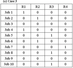
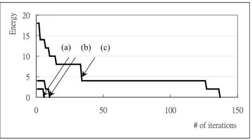
(15) Table 2. Timing Constraints Matrix. Figure 1 displays the energy curve of the best member in the population for 3 cases during iterations. The simulated scheduling results are graphically represented by using the. Energy. Gantt charts and are shown in Figure 2.. 20 15. (a). (b). (c). 10 5 0 0. 50. 100. 150 # of iterations. Fig. 1. The energy curve of the best member in the population.(a)Case 1 (b)Case 2 (c)Case 3..

(16) Fig. 2. The simulated scheduling results. (a)Case 1 (b)Case 2 (c)Case 3. 6. Conclusions In this paper, we present a GA-based approach with a feasible energy function to generate good-quality schedules. Unlike other schemes suffering from rapidly converging to the local optima, the genetic algorithms provide a better chance to obtain the global optima. Besides, a pure GA-based approach tends to generate illegal schedules due to the crossover and the mutation operators, it is often the case that the gene expression or the genetic operators need to be specially designed to fit the problem domain or some other schemes may be combined to solve the scheduling problems..

(17) In our work, we design an easy-understood genotype to generate legal schedules without modifying the genetic algorithm or genetic operators. Also, the energy function proposed work efficiently. The time required to obtain an optimal schedules using an exhaustive search increases exponentially with the augmentation of the number of jobs to be processed, the number of operations for each job and the number of flexible machines that can perform the processes. Therefore, the complexity of the search space is O(2N*2M*2T). However, in the three simulated cases, the proposed scheme converges rapidly. In the future, we attempt to investigate the applicability of our approach to larger-size practical examples. Reference [1] Yueh-Min Huang and Ruey-Maw Chen, “Scheduling Multiprocessor Job with Resource and Timing Constraints Using Neural Networks”, IEEE Transactions on Systems, Man and Cybernetics-Part B: Cybernetics, Vol.29, No.4, pp. 490-502, 1999. [2] Ruey-Maw Chen and Yueh-Min Huang, “Competitive Neural Network to Solve Scheduling Problems”, Neurocomputing, pp. 177-196, 2001. [3] Ruey-Maw Chen and Yueh-Min Huang, “Multiprocessor Task Assignment with Fuzzy Hopfield Neural Network Clustering Technique”, Neural Computing and Applications, pp. 12-21, 2001. [4] Ricardo C. Correa, Afonso Ferreira and Pascal Rebreyend, “Scheduling Multiprocessor Tasks with Genetic Algorithms”, IEEE Transactions on Parallel and Distributed Systems, Vol.10, No.8, pp. 825-837, 1999. [5] S. Hajri, N. Liouane, S. Hammadi and P. Borne, “A Controlled Genetic Algorithm by Fuzzy Logic and Belief Functions for Job-Shop Scheduling”, IEEE Transactions on Systems, Man and Cybernetics-Part B: Cybernetics, Vol.30, No.5, pp. 812-818, 2000. [6] Jian-Bo Yang, “GA-Based Discrete Dynamic Programming Approach for Scheduling in FMS Environments”, IEEE Transactions on Systems, Man and Cybernetics-Part B: Cybernetics, Vol.31, No.5, pp. 824-835, 2001. [7] Zbigniew Michalewicz, “Genetic Algorithms + Data structures = Evolution Programs”, Third Edition, Springer, pp. 13-44, 1999..

(18)